Aircraft-based inversions quantify the importance of wetlands and livestock for Upper Midwest methane emissions
←
→
Page content transcription
If your browser does not render page correctly, please read the page content below
Atmos. Chem. Phys., 21, 951–971, 2021
https://doi.org/10.5194/acp-21-951-2021
© Author(s) 2021. This work is distributed under
the Creative Commons Attribution 4.0 License.

Aircraft-based inversions quantify the importance of wetlands and
livestock for Upper Midwest methane emissions
Xueying Yu1 , Dylan B. Millet1 , Kelley C. Wells1 , Daven K. Henze2 , Hansen Cao2 , Timothy J. Griffis1 , Eric A. Kort3 ,
Genevieve Plant3 , Malte J. Deventer1,4 , Randall K. Kolka5 , D. Tyler Roman5 , Kenneth J. Davis6 , Ankur R. Desai7 ,
Bianca C. Baier8,9 , Kathryn McKain8,9 , Alan C. Czarnetzki10 , and A. Anthony Bloom11
1 Department   of Soil, Water, and Climate, University of Minnesota, Saint Paul, Minnesota 55108, United States
2 Department   of Mechanical Engineering, University of Colorado Boulder, Boulder, Colorado 80309, United States
3 Climate and Space Sciences and Engineering Department, University of Michigan, Ann Arbor,

Michigan 48109, United States
4 ANECO Institut für Umweltschutz GmbH & Co, 21079 Hamburg, Germany
5 Northern Research Station, US Department of Agriculture Forest Service, Grand Rapids, Minnesota 55744, United States
6 Department of Meteorology, The Pennsylvania State University, University Park, Pennsylvania 16802, United States
7 Department of Atmospheric and Oceanic Sciences, University of Wisconsin-Madison, Madison,

Wisconsin 53706, United States
8 Cooperative Institute for Research in Environmental Sciences, University of Colorado, Boulder,

Colorado 80309, United States
9 Global Monitoring Laboratory, National Oceanic and Atmospheric Administration, Boulder, Colorado 80305, United States
10 Department of Earth and Environmental Sciences, University of Northern Iowa, Cedar Falls, Iowa 50614, United States
11 Jet Propulsion Laboratory, California Institute of Technology, Pasadena, California 91109, United States

Correspondence: Dylan B. Millet (dbm@umn.edu)

Received: 5 August 2020 – Discussion started: 28 August 2020
Revised: 12 November 2020 – Accepted: 26 November 2020 – Published: 25 January 2021

Abstract. We apply airborne measurements across three sea-         pled soil temperature–hydrology effects is therefore needed.
sons (summer, winter and spring 2017–2018) in a multi-             Our optimized regional livestock emissions agree well with
inversion framework to quantify methane emissions from the         the Gridded EPA estimates during spring (to within 7 %)
US Corn Belt and Upper Midwest, a key agricultural and             but are ∼ 25 % higher during summer and winter. Spatial
wetland source region. Combing our seasonal results with           analysis further shows good top-down and bottom-up agree-
prior fall values we find that wetlands are the largest regional   ment for beef facilities (with mainly enteric emissions) but
methane source (32 %, 20 [16–23] Gg/d), while livestock            larger (∼ 30 %) seasonal discrepancies for dairies and hog
(enteric/manure; 25 %, 15 [14–17] Gg/d) are the largest an-        farms (with > 40 % manure emissions). Findings thus sup-
thropogenic source. Natural gas/petroleum, waste/landfills,        port bottom-up enteric emission estimates but suggest errors
and coal mines collectively make up the remainder. Opti-           for manure; we propose that the latter reflects inadequate
mized fluxes improve model agreement with independent              treatment of management factors including field application.
datasets within and beyond the study timeframe. Inversions         Overall, our results confirm the importance of intensive an-
reveal coherent and seasonally dependent spatial errors in         imal agriculture for regional methane emissions, implying
the WetCHARTs ensemble mean wetland emissions, with                substantial mitigation opportunities through improved man-
an underestimate for the Prairie Pothole region but an over-       agement.
estimate for Great Lakes coastal wetlands. Wetland extent
and emission temperature dependence have the largest in-
fluence on prediction accuracy; better representation of cou-

Published by Copernicus Publications on behalf of the European Geosciences Union.
952                                              X. Yu et al.: Aircraft-based inversions quantify the importance of wetlands

1   Introduction                                                   emission window, depending on location (Pickett-Heaps et
                                                                   al., 2011; Pugh et al., 2018; Knox et al., 2019; Peltola et al.,
Atmospheric methane (CH4 ) has increased global radiative          2019).
forcing by 0.97 W/m2 since 1750 (IPCC, 2013), making it               Livestock are the second-largest North American methane
the most important anthropogenic greenhouse gas after car-         source, accounting for an estimated ∼ 25 % of the total conti-
bon dioxide (CO2 ). Methane concentrations stabilized dur-         nental flux (∼ 35 % of the anthropogenic flux) during 2009–
ing the 1990s but resumed their increasing trend post-2007,        2011 (Turner et al., 2015). However, enteric and manure
with unclear causation (Kirschke et al., 2013; McNorton et         emissions vary strongly with animal type, diet, management,
al., 2018; Saunois et al., 2016; Thompson et al., 2018; Turner     and environmental factors (Niu et al., 2018; Charmley et al.,
et al., 2017, 2019; Dlugokencky et al., 2011). Prior work sug-     2016; Montes et al., 2013; Grant et al., 2015; Lassey, 2007;
gests that US emission increases account for 20 %–60 % of          VanderZaag et al., 2014), and top-down studies have revealed
the renewed global methane growth rate, with trends espe-          large uncertainties in the resulting source estimates. For ex-
cially large in the central US (Alvarez et al., 2018; Franco       ample, analyses of space-based, aircraft, and tall tower ob-
et al., 2016; Helmig et al., 2016; Maasakkers et al., 2019;        servations (Wecht et al., 2014; Miller et al., 2013) imply
Sheng et al., 2018a; Turner et al., 2016). Quantifying emis-       a 40 %–100 % underestimate of North American livestock
sions in this area is thus crucial for understanding the North     emissions in the EDGAR v4.2 and 2013 EPA inventories.
American methane budget and its role in driving global             Tall tower measurements similarly point to a 1.8-fold GEPA
trends. Here we employ new measurements from the GEM               livestock emission underestimate for the US Midwest (Chen
(Greenhouse Emissions in the Midwest) aircraft campaign            et al., 2018). Space-based methane retrievals from GOSAT
in a multi-inversion framework to develop constraints on           imply that US emissions rose by ∼ 20 % between 2010 and
methane emissions from the Upper Midwest region.                   2016, with a possible contribution from growing Midwest
   Recent studies imply uncertainties in the magnitude and         swine manure emissions (Sheng et al., 2018a). Previous stud-
distribution of North American methane emissions (Kirschke         ies have also revealed uncertainties in the spatial allocation
et al., 2013; Miller and Michalak, 2017; Dlugokencky et al.,       of US livestock methane emissions: the spatial R 2 between
2011). For example, Turner et al. (2015) found, based on           EDGAR v4.2 FT2010 and GEPA is only 0.5 for enteric fer-
measurements from the Greenhouse Gases Observing SATel-            mentation and 0.1 for manure management, with the mis-
lite (GOSAT), that the aggregated 2009–2011 US flux is             match for the latter most significant in the Upper Midwest
1.6× too low in the Emissions Database for Global Atmo-            (Hristov et al., 2017). A facility-based analysis of concen-
spheric Research (EDGAR v4.2, 2011; estimated US source            trated animal feeding operations in this area based on GEM
of 26 Tg/yr). However, subsequent work also using GOSAT            airborne data likewise pointed to spatial and temporal errors
retrievals (Maasakkers et al., 2019) concluded that the US         in bottom-up manure emissions (Yu et al., 2020).
flux is well-represented in the more recent Gridded Envi-             The Upper Midwest is a crucial region for atmospheric
ronmental Protection Agency inventory (GEPA Maasakkers             methane: its extensive wetlands and > 700 million live-
et al., 2016) – with a US flux just 12 % higher than that of       stock (USDA-NASS, 2018) have been estimated to ac-
EDGAR v4.2 – and argued that the inferred EDGAR biases             count for 30 % and 35 % of the total North American
may instead reflect spatial errors in that inventory. Surface      methane flux from wetlands and animal agriculture, re-
and aircraft-based inversion studies have further pointed to       spectively (Maasakkers et al., 2016; Bloom et al., 2017).
EPA bottom-up underestimates both nationally (Miller et al.,       The GEM study included extensive aircraft-based measure-
2013; Kort et al., 2008; Xiao et al., 2008; Karion et al., 2013;   ments of methane and related species across the Upper
Wecht et al., 2014; Caulton et al., 2014) and regionally (Chen     Midwest during three seasons (August 2017, January 2018,
et al., 2018).                                                     and May–June 2018, Fig. 1). The airborne sampling tar-
   Wetlands are thought to be the single largest North Amer-       geted wetland and agriculture emissions in particular, afford-
ican methane source (∼ 30 % of the total flux; Turner et al.,      ing a unique opportunity to advance understanding of these
2015), but there are major uncertainties in the magnitude and      sources. Here, we employ high-resolution chemical transport
spatiotemporal distribution of these emissions (Melton et al.,     modeling (GEOS-Chem chemical transport model (CTM) at
2013; Wania et al., 2013; Bruhwiler et al., 2014). For exam-       0.25◦ × 0.3125◦ ) in a multi-inversion framework (combining
ple, recent studies suggest an overestimate of wetland fluxes      sector-based, Gaussian Mixture Model and adjoint 4D-Var
in Canada and the southeastern US (Miller et al., 2016; Sheng      analyses) to interpret the GEM datasets in terms of regional
et al., 2018b) and that western Canadian and northern US           methane sources, with a focus on livestock and wetlands.
wetland emissions have a broader spatial distribution than is
predicted by models (Miller et al., 2014). Northern wetland
emissions have strong seasonality, with a typical onset in late
spring, peak in July–August, and decline in the fall with the
onset of freezing. Bottom-up models have been shown to
both underpredict and overpredict the width of this seasonal

Atmos. Chem. Phys., 21, 951–971, 2021                                                 https://doi.org/10.5194/acp-21-951-2021
X. Yu et al.: Aircraft-based inversions quantify the importance of wetlands                                                       953

Figure 1. GEM flight tracks and additional datasets used in this study. Panel (a) shows Pacific flight tracks for the ATom3 and ATom4
campaigns used for evaluating modeled boundary and initial conditions. Also shown are the ACT-America flight tracks (C130 in cyan, B200
in red) used here for posterior model evaluation. The inner red box (40–50◦ N, 87–100◦ W) shows the GEM flight region that is expanded
in (b–d), the black box (35–55◦ N, 80–105◦ W) shows the Upper Midwest analysis region employed for source inversions, and the blue box
(9.75–60◦ N, 60–130◦ W) demarks the GEOS-Chem nested North American domain. The right panels show the GEM flight tracks colored
by observed methane mixing ratios and superimposed on the prior annual bottom-up emissions described in-text. Also shown are locations
for the radiosonde launches and tall towers employed here, along with the Bog Lake peatland eddy flux site.

2     Data and methods                                                strumental precision for methane is < 1 ppb, and the over-
                                                                      all accuracy is estimated at < 3.5 ppb based on the expanded
2.1    GEM flights and measurement payload                            uncertainties for the calibration standard. We use 1 min av-
                                                                      eraged observations here to constrain regional fluxes. Addi-
The GEM aircraft campaign was designed to survey regional             tional onboard observations included nitrous oxide (N2 O),
methane sources via downwind and upwind transects. Fig-               carbon monoxide (CO), H2 O, and CO2 mole fractions by
ure 1 shows sampling tracks, including 23 flights (156 h)             continuous-wave tunable infrared laser absorption spectrom-
across three seasons (GEM1: 8 flights, 12–24 August 2017;             etry (0.5 Hz, Aerodyne Research Inc., USA) as described
GEM2: 7 flights, 17–28 January 2018; GEM3: 8 flights,                 by Gvakharia et al. (2018); ozone (O3 ) mole fractions
21 May–2 June 2018). Flights ranged from 4–8 h in duration            (0.2 Hz; dual-beam ultraviolet spectrometer, model 205, 2B
(mean: 6 h) and took place in the daytime mixed layer (be-            Technologies Inc., USA); temperature and relative humidity
tween 10:00 and 19:00 local standard time, 200–600 m a.g.l.)          (1 Hz; model HMP60, Vaisala Corp., Finland); and GPS lo-
onboard a Mooney aircraft with ∼ 280 km/h boundary layer              cation, wind speed and direction, ambient pressure, and other
cruise speed (Scientific Aviation Inc.). Tracks were selected         relevant flight parameters as described by Yu et al. (2020).
and optimized on the day of flight (avoiding light, variable,
or shifting winds; poorly developed mixed layers; and frontal         2.2     Forward modeling framework
systems) to minimize analysis errors due to uncertain mete-
orology. Along with mixed-layer surveying, each flight in-            2.2.1    GEOS-Chem methane simulation and prior
cluded 1–2 vertical profiles to characterize the atmosphere’s                  emissions
vertical structure from the surface to lower free troposphere.
The GEM flights also included extensive point source char-            We use the GEOS-Chem CTM (v11-02; http://acmg.seas.
acterization as described by Yu et al. (2020).                        harvard.edu/geos, last access: 11 January 2021) and its ad-
   A cavity ring-down spectrometer (CRDS G2301 for                    joint (v35) to optimize regional methane emissions. Sim-
GEM1, G2210-m for GEM2 and GEM3; Picarro Inc., USA)                   ulations are performed on a nested 0.25◦ × 0.3125◦ grid
was deployed on the aircraft to quantify methane, ethane              over North America (9.75–60◦ N, 60–130◦ W; Fig. 1) using
(C2 H6 , GEM2 and GEM3 only), water vapor (H2 O) and car-             GEOS-FP meteorological fields from the National Aeronau-
bon dioxide (CO2 ) mole fractions at 1 Hz. Ground-based cal-          tics and Space Administration (NASA) Global Modeling and
ibrations employed compressed ambient-level gas cylinders             Assimilation Office (GMAO, 2013), with 5 and 10 min time
traceable to National Oceanic and Atmospheric Administra-             steps for transport and emissions, respectively. The 3-hourly
tion (NOAA) Global Monitoring Laboratory (GML) stan-                  dynamic boundary conditions (BC) are from global simula-
dards on the WMO X2004A CH4 calibration scale. The in-                tions at 2◦ × 2.5◦ and bias-corrected as described later. Ini-

https://doi.org/10.5194/acp-21-951-2021                                                   Atmos. Chem. Phys., 21, 951–971, 2021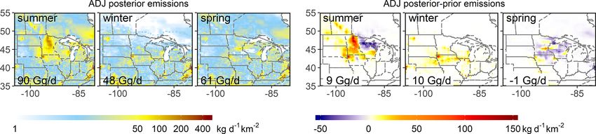
954 X. Yu et al.: Aircraft-based inversions quantify the importance of wetlands
tial conditions are obtained from a 25-year global spin-up 2.2.2 Evaluating model boundary and initial conditions
at 2◦ × 2.5◦ (bias-corrected in the same manner), followed
by a 30 d high-resolution (0.25◦ × 0.3125◦ ) spin-up over our Given the large atmospheric methane burden (1850–
nested domain. 1950 ppb) relative to the magnitude of North American en-
Prior methane emissions in the model are as follows. Wet- hancements (up to 200 ppb in our prior simulations), careful
land emissions use the WetCHARTs ensemble mean (Bloom background evaluation is needed to avoid a biased source op-
et al., 2017), uniformly scaled up by 10 % to match the timization. We therefore use measurements over the remote
global estimate from Kirschke et al. (2013). Anthropogenic Pacific from the Atmospheric Tomography Mission (ATom;
emissions use the GEPA inventory (Maasakkers et al., 2016) flight tracks shown in Fig. 1) to evaluate and correct the
over the US (which includes seasonally varying livestock model boundary and initial conditions. ATom featured pole-
and rice emissions and aseasonal fossil fuel, waste, and in- to-pole sampling with continuous vertical profiling (0.2–
dustrial emissions). Anthropogenic emissions elsewhere are 12 km) and onboard measurements including methane (Pi-
based on EDGAR v4.3.2 (2017), except Canadian and Mex- carro model G2401m, Picarro Inc., USA) and a wide suite of
ican oil and gas emissions, which use CanMex (Sheng et al., other atmospheric species (Wofsy et al., 2018).
2017). Emissions from biomass burning use the Quick Fire Figure S1 compares tropospheric background methane
Emissions Dataset (QFED) (Darmenov and Silva, 2015), and measurements (represented as 0.1 quantiles within 1◦ lat-
those from geological seeps and termites follow Maasakkers itude bins) from ATom3 (September–October 2017; flight
et al. (2019) and Fung et al. (1991), respectively. Simulations altitudes ≤ 10 km) and ATom4 (April–May 2018; flight al-
include a set of tagged tracers to track methane from relevant titudes ≤ 8 km) with GEOS-Chem predictions along the
source sectors as detailed in Sect. 2.3. flight tracks. The model–measurement background differ-
Our analyses focus on the Upper Midwest, defined here ence over North American latitudes averages 5.4 ppb (0.3 %)
to include the north central US and south central Canada re- for ATom3 and 9.2 ppb (0.5 %) for ATom4. We correct the
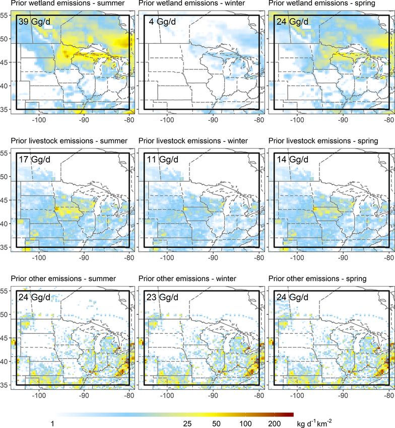
gion shown in Fig. 1. Figure 2 maps the prior emissions for model boundary and initial conditions using a smoothed
summer, winter and spring. According to the above invento- spline fit of this 0.1 quantile difference to latitude, with
ries, wetlands (36 % of the total annual flux) and livestock GEM1 (July–August 2017) and GEM2 (January 2018) cor-
(23 %) represent the two largest regional methane sources. rected based on ATom3 and GEM3 (May–June 2018) cor-
Natural gas and petroleum systems, wastewater and land- rected based on ATom4.
fills, coal mines, and other sources contribute the remain- Finally, as described later we assess the potential impact of
ing 15 %, 12 %, 9 %, and 5 %, respectively. Seasonality in any residual model background errors through a set of sensi-
the prior emissions is dominated by wetlands; these vary tivity inversions in which the bias-corrected boundary condi-
from 39 Gg/d in July–August 2017 (GEM1) to 4 Gg/d in Jan- tions are included in the state vector for further optimization.
uary 2018 (GEM2), with an onset in late May during the Results are described in Sect. 2.5 and employ a 0.4 % back-
GEM3 timeframe. The prior livestock emissions vary from ground error standard deviation based on the above model–
17 Gg/d in July–August 2017 (GEM1) to 11 Gg/d in Jan- measurement disparities.
uary 2018 (GEM2) due to the temperature-dependent manure
source. Figure 2 shows that wetland emissions are concen- 2.2.3 Assessing meteorological uncertainties
trated in the north of the Upper Midwest domain, whereas
livestock and other anthropogenic emissions occur predom- We use two approaches to assess the potential impacts
inantly to the south. This spatial separation provides an im- of model transport errors on our findings. First, we test
portant advantage for resolving source contributions in our whether a misrepresentation of regional-scale synoptic trans-
inversions. port could bias our inversion results by evaluating the op-
The major atmospheric methane sink (90 % of the total timized model against independent datasets from different
loss) is oxidation by hydroxyl radical (OH), computed in the years, as described in Sect. 2.4. Second, we assess model
model using archived 3-D monthly OH fields from a full- uncertainties in vertical mixing using planetary boundary
chemistry simulation (v5-07-08). Other loss processes in- layer (PBL) depth estimates derived from balloon-based
clude stratospheric oxidation (6 % of the total sink), com- radiosonde profiles in the Integrated Global Radiosonde
puted using archived monthly loss frequencies from the Archive Version 2 (IGRA v2). We use 00:00 UTC (18:00 or
NASA Global Modeling Initiative (Murray et al., 2013); soil 19:00 local standard time) sonde launch data from six sites in
absorption (3 %), computed following Fung et al. (1991); and the Upper Midwest (Fig. 1, red triangles) during August 2017
tropospheric oxidation by chlorine (Cl, 2 %), computed using (GEM1), January 2018 (GEM2), and May 2018 (GEM3) in
archived 3-D monthly Cl fields from Sherwen et al. (2016). this analysis. Depending on season, the 00:00 UTC sound-
The resulting global tropospheric methane lifetime in our ing can occur after the collapse of the daytime mixed layer,
simulations is 12 years. but the preceding day’s PBL depth can still generally be de-
termined from vertical temperature and dew point transitions
atop the residual layer. The resulting PBL estimates are then
Atmos. Chem. Phys., 21, 951–971, 2021 https://doi.org/10.5194/acp-21-951-2021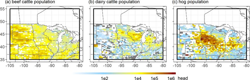
X. Yu et al.: Aircraft-based inversions quantify the importance of wetlands                                                             955

Figure 2. Prior methane emissions in the Upper Midwest for the GEM 1–3 flight periods (GEM1 – summer, 20 July–24 August 2017; GEM2
– winter, 3–28 January 2018; GEM3 – spring, 7 May–2 June 2018). Emission inventories are as described in the text. The black box indicates
the inversion domain.

compared with the mean midday (12:00–16:00) value in the               sions employ widely differing assumptions and constraints,
model. Figure S2 shows that the resulting model PBL biases             and together they allow us to identify robust aspects of the
average less than 10 %, with mean model:measurement ra-                derived methane flux fields and quantify the sensitivity of
tios of 0.98, 0.97 and 0.90 for summer, winter and spring, re-         results to these assumptions. We perform the above inver-
spectively. While the GEOS-FP daytime mixing heights were              sions separately for each season (summer: GEM1; winter:
shown previously to be biased high (by 30 %–50 %) over the             GEM2; spring: GEM3). Inversion performance is discussed
US Southeast during summer (Millet et al., 2015), we find              in Sect. 2.5.
here that no such bias manifests over the Upper Midwest.
                                                                       2.3.1   Cost function and error specification
2.3   Inverse modeling framework
                                                                       All inversions in this study optimize methane emissions by
We quantify methane emissions in the Upper Midwest us-                 minimizing the Bayesian cost function J (x):
ing a multi-inversion framework that combines (1) sector-
                                                                                                                        T −1
based analytical inversions, with the prior spatial distribution       J (x) = (x − x a )T S−1
                                                                                            a (x − x a ) + γ (y − F (x)) SO ( y − F (x)),
of emissions taken as a hard constraint; (2) spatial and sec-                                                                               (1)
toral clustering of grid cells using a Gaussian Mixture Model
(GMM), with subsequent analytical optimization; and (3) ap-            where x is the state vector to be optimized (defined differ-
plication of the GEOS-Chem adjoint to spatially optimize               ently for the various inversion frameworks), x a is the vector
fluxes on the 0.25◦ × 0.3125◦ model grid. The above inver-             of prior emissions, Sa is the error covariance matrix for the

https://doi.org/10.5194/acp-21-951-2021                                                     Atmos. Chem. Phys., 21, 951–971, 2021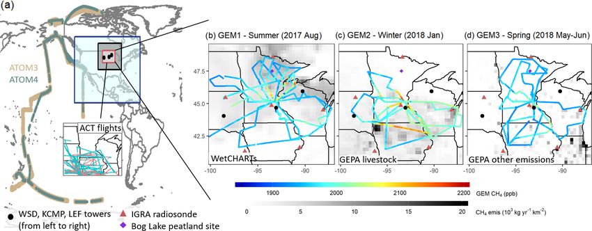
956                                              X. Yu et al.: Aircraft-based inversions quantify the importance of wetlands

prior emissions, y and F (x) are the observed and simulated        mites). Over the timescale and spatial scale of our inversions
methane mixing ratios along the GEM flight tracks, respec-         the methane emission–concentration relationship is linear,
tively, and SO is the error covariance matrix for the observ-      and we thus construct the Jacobian matrix K using tagged
ing system (including both measurement and model contri-           tracers for each of the above source sectors. The sector-based
butions). The regularization parameter γ balances the prior        inversions offer the advantage of direct source attribution but
and observational contributions to J (x) and is set to 10 for      with increased potential for aggregation error given the pre-
our base-case analyses as discussed in the Supplement.             scribed emission distributions.
   Prior errors are prescribed as follows. Wetland emission
uncertainties are based on the standard deviation (σ ) of          2.3.3   GMM inversions
the WetCHARTs ensemble on the 0.25◦ × 0.3125◦ model
grid, averaging 140 % for summer (σ = 55 Gg/d) and spring          The GMM inversions cluster individual (∼ 25 km) grid cells
(σ = 34 Gg/d) and 310 % for winter (σ = 12 Gg/d) on the            with similar emission characteristics, and then analytically
Upper Midwest domain of Fig. 1. For anthropogenic emis-            optimize methane fluxes by cluster. GMM is a probabilis-
sions, we employ a scale-dependent uncertainty (encom-             tic approach that assumes each subpopulation (or cluster)
passing magnitude and displacement uncertainties) follow-          is a multivariate Gaussian distribution (i.e., each cluster is
ing Maasakkers et al. (2016); the resulting error standard de-     ellipsoidal and centered in the feature space) (Turner and
viation averages 40 %–105 % across sectors over our study          Jacob, 2015). We use an expectation-maximization algo-
region. For other sources we assume a prior error standard         rithm (Dempster et al., 1977) to find the maximum-likelihood
deviation of 50 % following earlier studies (Maasakkers et         GMM classification for seven emission sectors in the Upper
al., 2019; Turner et al., 2015; Wecht et al., 2014; Zhang et       Midwest (wetland, livestock, fossil fuel, rice, biomass burn-
al., 2018; Sheng et al., 2018b). For inversions optimizing the     ing, other anthropogenic emissions and other natural emis-
total methane flux across sectors, the above terms are com-        sions) and for total emissions in other regions. In each case
bined in quadrature as the diagonal elements of the prior error    the number of clusters 0 ∈ [1, 9] is selected based on the
covariance matrix.                                                 Bayesian Information Criterion (Schwarz, 1978), with low-
   The adjoint 4D-Var inversions derive methane emissions at       emission clusters (e.g., termites and seeps) grouped to avoid
0.25◦ × 0.3125◦ resolution, and in this case we use a 200 km       weak sensitivity in the Jacobian matrix. Sector-specific clus-
length scale (decaying exponentially) to populate the off-         ters in the Upper Midwest are defined using eight mean- and
diagonal elements of the prior error covariance matrix. Pre-       variance-normalized variables: latitude, longitude, grid-level
vious methane inversions by Wecht et al. (2014) and Monteil        prior sectoral emissions (three seasons) and grid-level scal-
et al. (2013) assumed length scales of 275–500 km to further       ing factors (SFs; iteration 8; three seasons) derived from the
smooth the solution. In our case the analytical inversions im-     adjoint 4D-Var inversions. Emission clusters for other re-
pose strict error correlation by spatial cluster or source sec-    gions are defined using the above eight variables (for total
tor; thus, the adjoint and analytical analyses together span a     emissions) and the prior sectoral emission fractions (seven
wide range of error correlation scenarios. Since the analyti-      sectors × three seasons). In this way we identify a total of
cal inversions solve for emissions by sector or by aggregated      28 GMM clusters (Fig. S3), construct the Jacobian matrix
region, we employ diagonal prior errors in those cases.            K based on the associated sensitivities in simulations with
   The observational error covariance matrix is constructed        tracers tagged to these 28 clusters and solve dJ (x) /dx an-
from the residual standard deviation of the observation–prior      alytically. The GMM inversions thus derive sector-resolved
model difference across a 2◦ × 2◦ moving window (Heald             methane fluxes along with their general spatial distributions.
et al., 2004). The resulting error standard deviation, includ-     They provide a middle ground between the source-resolved
ing forward model and instrumental contributions, averages         but spatially constrained sector-based inversions above and
26 ppb and is assumed diagonal. The overall observing sys-         the spatially resolved but source-agnostic adjoint 4D-Var in-
tem error is hence dominated by forward model and repre-           versions below.
sentation errors rather than by the < 1 ppb measurement pre-
cision.                                                            2.3.4   Adjoint 4D-Var inversions

2.3.2   Sector-based inversions                                    The adjoint 4D-Var inversions optimize total methane emis-
                                                                   sions on the 0.25◦ × 0.3125◦ model grid via iterative mini-
We first derive an optimized set of methane emissions by           mization of dJ (x) /dx in a quasi-Newtonian routine (Henze
solving dJ (x) /dx analytically by sector. Seven state vec-        et al., 2007). The resulting state vector contains 6400 ele-
tor elements are thus optimized across the nested model do-        ments over the Upper Midwest domain (Fig. 1), thus en-
main, representing emissions from (1) wetlands, (2) live-          abling detailed spatial corrections to the prior emissions on
stock, (3) fossil fuel, (4) rice, (5) biomass burning, (6) other   a ∼ 25 km scale. To avoid overfitting, we impose a 200 km
anthropogenic emissions (landfill, waste water, and other)         prior error correlation length scale as described previously.
and (7) other natural emissions (geological seeps and ter-         We further perform a suite of sensitivity inversions to eval-

Atmos. Chem. Phys., 21, 951–971, 2021                                                 https://doi.org/10.5194/acp-21-951-2021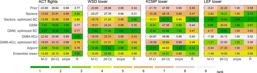
X. Yu et al.: Aircraft-based inversions quantify the importance of wetlands                                                957

uate the robustness of the derived emissions by varying the          during summer and spring. In winter, livestock (43 %)
initial scale factors (i.e., employing the GMM-derived scale         and fossil fuel (41 %) sources predominate.
factors as the initial guess in the adjoint optimization, re-
ferred to as GMM-ADJ in the following) and by varying the        3. KCMP tall tower measurements. Methane is mea-
regulation parameter γ ∈ [0.1, 1000] and thereby the weight         sured at KCMP (Rosemount, Minnesota; 44.69◦ N,
of the prior versus observational cost function terms. In all       93.07◦ W, 290 m a.s.l.; AMERIFLUX, 2018; Chen et
cases convergence to the final result is ascertained based on       al., 2018) by tunable-diode laser absorption spec-
a cost function reduction per iteration < 2.5 % of J0 .             troscopy (TGA200A, Campbell Scientific Inc., USA)
                                                                    from two air sampling inlets at 3 and 185 m a.g.l.
2.4   Independent measurements for evaluation                       The KCMP tower is located 25 km south of the
                                                                    Minneapolis–Saint Paul metropolitan area and sam-
We evaluate our top-down methane emission estimates us-             ples a predominantly agricultural footprint (easterly,
ing the independent airborne and tall tower datasets shown          southerly and westerly winds), along with urban
in Fig. 1 and described below. Datasets are calibrated using        and wetland influences (northerly winds). The main
standards traceable to the WMO X2004A calibration scale,            methane source influences at KCMP according to
with overall accuracies < 4 ppb in all cases (Davis et al.,         the prior GEOS-Chem simulations are from wetlands
2018; Andrews et al., 2017; Richardson et al., 2017). Com-          (50 %–56 % of the mean simulated enhancement) and
parisons are based on 5 s (aircraft) and 1 h (tower) averaged       livestock (22 %) during spring and summer and from
data, with the model sampled at the time and location of mea-       livestock (39 %) and fossil fuel (27 %) during winter.
surement.
                                                                 4. LEF tall tower measurements. Methane is measured
 1. ACT-America airborne measurements. The Atmo-                    at LEF (Park Falls, Wisconsin; 45.95◦ N, 90.27◦ W,
    spheric Carbon and Transport-America (ACT-America)              470 m a.s.l.; Desai et al., 2015; Andrews et al., 2017)
    campaign (Davis et al., 2018; DiGangi et al., 2017)             by cavity-enhanced absorption spectroscopy (LGR 908-
    featured methane measurements from two aircraft plat-           0001 Fast Methane Analyzer, Los Gatos Research,
    forms, in both cases by CRDS (2401 m, Picarro Inc.,             Inc., USA). Measurements are performed sequen-
    USA) at 1 Hz frequency (Davis et al., 2018; Baier et al.,       tially from three air sampling inlets at 30, 122 and
    2020). We employ within-PBL methane observations                396 m a.g.l. based on the protocol described by Andrews
    from ACT-America flights during July–August 2016,               et al. (2014). The LEF tower is located in the northeast
    October–November 2017 and April–May 2018 to eval-               of our analysis region within a mixed wetland and forest
    uate GEM inversion results for summer, winter and               landscape. LEF features a larger influence from natural
    spring, respectively. The 5 s average measurements and          emissions than the datasets above: based on our prior
    along-track model output are both aggregated to the             simulations, wetlands contribute > 67 % of the mean
    model grid and time step prior to intercomparison.              methane enhancement during summer and spring (ver-
    Flights selected for inversion evaluation occurred over         sus 44 %–56 % for the other tall towers); livestock con-
    and downwind of the Upper Midwest (Fig. 1), mainly              tribute an additional 15 %. In winter, fossil fuels (34 %)
    sampling the southern portion of our domain. Live-              and livestock (31 %) drive the largest concentration en-
    stock (29 % of the mean simulated enhancement), fossil          hancements.
    fuel (28 %) and wetlands (26 %) are the three largest
    methane source influences along these flight tracks            In the case of the tall tower measurements, we use two
    based on the prior GEOS-Chem tagged tracer simula-          approaches to evaluate our inversion results. First, we test
    tions.                                                      the optimized model against tall tower data contempora-
                                                                neous with the GEM flights (August 2017, January 2018,
 2. WSD tall tower measurements. Methane is measured at         May 2018). Second, we test the optimized model against
    WSD (Wessington, South Dakota; 44.05◦ N, 98.59◦ W,          tall tower data for the same month in a different year (Au-
    592 m above sea level (a.s.l.); Miles et al., 2018)         gust 2018, January 2017, May 2017). The latter test guards
    by CRDS (CFADS2401 or CFADS2403; Picarro Inc.,              against overfitting to the GEM data; for example, erro-
    USA) from a single inlet at 60 m above ground level         neously adjusting emissions to compensate for broadscale
    (a.g.l.). The WSD tower is located in the southwest of      model transport errors during the GEM timeframe. In both
    our analysis region, and thus captures the influence of     cases we employ daytime (10:00–18:00 LT) data for model–
    long-range transport under westerly winds and of Up-        measurement comparison. The WSD tower was not yet es-
    per Midwest emissions under easterly winds. Based on        tablished in January 2017, and thus only the later compar-
    the prior tagged tracer simulations, wetlands (45 % of      isons are possible here. In all cases we use observations from
    the mean simulated enhancement) and livestock (30 %)        the highest available inlet, with the model sampled at the cor-
    are the two largest methane source influences at WSD        responding vertical level, to ensure the widest fetch for sam-

https://doi.org/10.5194/acp-21-951-2021                                            Atmos. Chem. Phys., 21, 951–971, 2021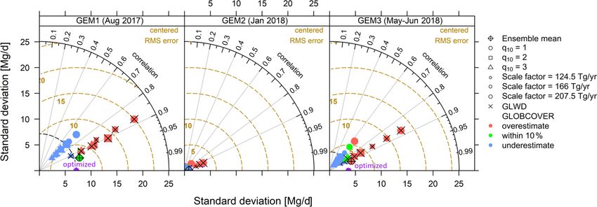
958                                               X. Yu et al.: Aircraft-based inversions quantify the importance of wetlands

pling regional emissions while minimizing near-field influ-          livestock estimates are not strongly sensitive to fossil fuel-
ences.                                                               related emission errors and that (ii) the derived oil and gas
                                                                     fluxes are prior-dependent and only weakly constrained by
2.5   Inversion performance                                          the GEM observing system.
                                                                        In nearly every case, the simulations with optimized emis-
All inversions lead to a significant reduction in the cost func-     sions agree more closely with independent aircraft and tall
tion, with the adjoint 4D-Var and GMM inversions tending             tower measurements than the prior simulations do (Fig. 4).
to yield larger decreases (36 %–97 %) than the sector-based          Exceptions include (i) the sector-based inversion versus the
inversions (12 %–43 %). The adjoint 4D-Var and GMM in-               WSD tower data and the GMM-ADJ inversion versus the
versions are able to optimize the spatial distribution of emis-      KCMP and LEF tower data. The former likely reflects ag-
sions, improving the posterior fit to the data and reducing          gregation error in the spatially constrained sectoral optimiza-
aggregation error.                                                   tion. The latter suggests overfitting: the GMM-ADJ emission
   Figure 3 shows that the derived adjustments to the total          adjustments improve model performance during the GEM
regional methane flux are consistent across inversion frame-         timeframe (Fig. S4) but not for alternate years (Fig. 4). For all
works. Specifically, results point to a wintertime emission          other inversions, the optimized emissions yield performance
underestimate and to very modest (< 10 %) springtime cor-            improvements regardless of the evaluation year, providing a
rections. More variable results are obtained during summer;          strong argument for the representativeness of the GEM data
however, even here the derived total flux adjustments are            and the reliability of our emission adjustments.
≤ 23 % in all cases.                                                    Together, the ensemble of inversions provides an envelope
   The sector-based and GMM inversions enable direct                 of solutions for assessing the robustness and uncertainty of
source attribution, and we attribute the adjoint-derived emis-       the results. Below, we discuss emergent findings that are con-
sions based on the prior grid cell source fractions. We find in      sistent across inversions and diagnose the associated level of
this way that (as with the total flux) inversion results are also    confidence based on the spread in results.
generally consistent on a sectoral level: uniformly upward
adjustments are derived in winter, whereas springtime results
point to a wetland overestimate but to only minor correc-
tions for other sources. As before, sectoral results are more        3     Optimized methane emissions in the Upper Midwest
variable during summertime; this point is further discussed
below. Finally, we show later that geographically consistent         Averaging our seasonal inversion results with the prior values
emission adjustments are obtained across the set of spatially        for fall, we find that wetlands represent the single largest (32
explicit inversions, further supporting the robustness of our        [29–35] %) methane source in the Upper Midwest at 20 [16–
findings.                                                            23] Gg/d. Here and below, reported central values and uncer-
   The largest disparities in Fig. 3 occur when the methane          tainties reflect the mean and range across our inversion en-
boundary conditions are optimized in the inversion rather            semble. Anthropogenic sources collectively account for the
than prescribed: total regional emissions derived in this way        remaining 68 [65–71] %, with livestock making the largest
are ∼ 15 %–25 % lower than the ensemble mean during sum-             individual contribution (15 [14–17] Gg/d). Smaller but still
mer and winter. The summertime wetland emissions exhibit             significant sources are derived for natural gas and petroleum
the strongest such sensitivity, reflecting imperfect seasonal        systems (10 [9–11] Gg/d), waste and landfills (8 [7–8] Gg/d),
wetland–background separation in the GEM data. In particu-           and coal mines (6 [5–7] Gg/d); however, as noted above these
lar, the only downward adjustments (up to 34 %) to the sum-          latter estimates are strongly influenced by the prior. Given
mer wetland flux are derived when optimizing boundary con-           the predominant role for livestock and wetlands, we focus on
ditions; all other inversions yield ≤ 24 % positive corrections.     these sources and proceed to discuss the above findings in
These same disparities account for the largest spread in de-         detail by season.
rived total flux estimates for summer (scale factors of 0.85
versus 1.23). We show below that inclusion of the boundary           3.1    Summer (GEM1): spatial errors in the prior
conditions in the state vector for optimization does not con-               wetland flux and an underestimate for livestock
sistently improve model performance, supporting the prior
use of ATom data for this purpose.                                   Figure 3 shows that the GEM aircraft data broadly sup-
   We performed a series of sensitivity inversions to test how       port the total prior summertime methane emissions for the
our results depend on the weighting of the observational ver-        Upper Midwest, with a derived correction factor of 1.10
sus prior components of the cost function, the prior wetland         [0.85–1.23]. The resulting posterior seasonal flux is 88 [68–
emissions, and the prior oil and gas emissions. Results are          99] Gg/d. On a sectoral basis, wetlands provide the dominant
detailed in the Supplement and show that our overall findings        seasonal emission source (45 %, 39 [26–49] Gg/d). Livestock
are robust across these tests. In the case of the oil and gas sen-   account for 24 % (21 [18–24] Gg/d), with the remaining 31 %
sitivity analysis, we find in particular that (i) our wetland and    (27 [24–32] Gg/d) including a derived 16 [14–21] Gg/d from

Atmos. Chem. Phys., 21, 951–971, 2021                                                   https://doi.org/10.5194/acp-21-951-2021
X. Yu et al.: Aircraft-based inversions quantify the importance of wetlands                                                           959

Figure 3. Methane emission scale factors by sector derived from the multi-inversion analysis over the Upper Midwest (black box in Fig. 1).
Results are shown for GEM1 (a, b; July–August 2017), GEM2 (c, d; January 2018) and GEM3 (e, f; May–June 2018). Matrix columns
show aggregated regional scale factors for total methane emissions (TOTAL), livestock (LIV), wetlands (WTL), and other sources (OTH).
Rows show results from seven individual inversions (for details, see Sect. 2.3) along with the ensemble mean. Bar plots in the top row show
the emission fractions for each source grouping based on the ensemble-mean inversion results. Boundary condition scale factors for the
corresponding sector-based and GMM inversions are 1.00/1.02 (summer), 1.00/1.01 (winter) and 1.00/1.00 (spring), respectively.

Figure 4. Inversion performance evaluation against independent observations from alternate years. Evaluation datasets include airborne mea-
surements from the ACT-America campaign and tall tower measurements from Wessington South Dakota (WSD), Rosemount Minnesota
(KCMP), and Park Falls Wisconsin (LEF). Each matrix displays summary performance statistics for the seven inversions, and for the ensem-
ble mean, with respect to the indicated evaluation dataset. Columns in each matrix show the model mean bias (M-O; ppb), mean absolute
bias (|M-O|; ppb), model:measurement slope (note this is within 1 % of unity in all cases) and model:measurement Pearson’s correlation
coefficient (R). Values are colored by rank for the above criteria. See Sect. 2.4 for details.

fossil fuels (including coal mines) and 8 [8–9] Gg/d from               ual inversions reveal a wetland underestimate in the north-
wastewater.                                                             west of our domain (reaching 76 mg/m2 /d) but an overesti-
   While the optimized summertime wetland fluxes agree                  mate in the northeast (reaching −77 mg/m2 /d). These spatial
reasonably well with the WetCHARTs estimate for the re-                 patterns are robust across the inversions, but the adjustment
gion as a whole (mean scale factor of 1.00 [0.66–1.24]), this           magnitudes differ – for example, the GMM inversion yields
is fortuitous: the inversions point to significant (offsetting)         much stronger upward adjustments in the northwest (Figs. 5–
spatial errors in the prior. Figures 5–7 show that the individ-

https://doi.org/10.5194/acp-21-951-2021                                                      Atmos. Chem. Phys., 21, 951–971, 2021
960                                            X. Yu et al.: Aircraft-based inversions quantify the importance of wetlands

7). We attribute this spread in part to the imperfect wetland–   role of enteric fermentation versus manure management in
background separation discussed earlier.                         driving these differences.
   The northwest wetlands lie predominantly in the Prairie          The wintertime optimization results further point to a 28
Pothole region of the eastern Dakotas and Canada and have        [9–45] % (6 [2–10] Gg/d) underestimate of non-livestock an-
highly variable hydrology driven by snowmelt, precipita-         thropogenic emissions, with the largest derived adjustments
tion, and groundwater inflow. Based on 1997–2009 data,           in the southeast of our domain where fossil fuel sources
these wetlands have been declining at a rate of ∼ 25 km2 /yr     predominate (Figs. 5–7). Sustained high methane observa-
(USF&WS National Wetlands Inventory, 2019). Areas to the         tions during a GEM2 flight over Iowa under southerly winds
northeast mainly feature coastal wetlands under the influence    (Fig. 1) – with up to 100 ppb model–measurement mis-
of the Great Lakes, which based on 2004–2009 data have           matches and co-occurring ethane enhancements – similarly
undergone recent expansion by 11 km2 /yr (USF&WS Na-             suggest an underestimate of fossil fuel sources to the south
tional Wetlands Inventory, 2019). Our findings here suggest      of the Upper Midwest, as also diagnosed by Barkley et
that methane emissions from Great Lake coastal wetlands          al. (2019). However, for the purpose of analyses here, we
(while increasing over time) are presently overestimated,        note that a sensitivity inversion omitting this flight does not
while prairie pothole emissions (while decreasing over time)     significantly alter our results.
are presently underestimated.
   We further infer from the GEM aircraft measurements a
                                                                 3.3   Spring (GEM3): biased seasonal onset of wetland
summertime underestimate in regional anthropogenic emis-
                                                                       emissions
sions (Fig. 3). In particular, the GEPA prior livestock emis-
sions increase by 24 % (4 Gg/d) in the multi-inversion aver-
age, with scale factors ranging from 1.05–1.41 (1–7 Gg/d).       The GEM aircraft data indicate that the prior regional flux
As seen earlier for wetlands, the lowest scale factors (1.05,    during springtime is unbiased when taken as a whole: Fig. 3
1.07) are obtained when the boundary conditions are allowed      shows that the ensemble mean correction factor is 1.01 with
to vary in the optimization, with other inversions point-        a range across inversions of 0.95–1.10, resulting in a spring
ing to a 21 %–41 % (4–7 Gg/d) livestock flux underestimate.      flux of 63 [59–68] Gg/d. On a sectoral basis, wetlands are the
The individual inversions are spatially consistent in showing    largest emission source (33 %, 21 [16–25] Gg/d), followed
the livestock underestimate manifesting most strongly in the     by livestock (24 %, 15 [14–16] Gg/d), with the remainder in-
center of the Upper Midwest domain (Iowa/southern Min-           cluding derived contributions of 16 [14–17] Gg/d from fossil
nesota/southern Wisconsin; Figs. 5–7). Anthropogenic emis-       fuel and 9 [8–9] Gg/d from wastewater.
sions other than livestock are adjusted upward through the          While the GEM inversions support the prior springtime
inversions by 15 [1–35] % (4 [0–8] Gg/d) in a relatively con-    methane fluxes in terms of total regional magnitude, results
sistent manner across the region (Figs. 5–7).                    point to biases in the bottom-up wetland emissions and their
                                                                 spatial distribution. Figures 5–7 show that the prior wetland
                                                                 emissions during spring exhibit spatial errors similar to those
3.2   Winter (GEM2): an emission underestimate across
                                                                 in summer, with an underestimate to the northwest (reach-
      sectors
                                                                 ing 15 mg/m2 /d) but an overestimate around the Great Lakes
                                                                 (reaching −48 mg/m2 /d). These spatial errors have smaller
All inversions indicate that wintertime methane emis-            peak magnitude (< 63 %) than during summer and lead to a
sions are underestimated in the prior inventories, with an       net 15 % wetland flux overestimate for the region as a whole
ensemble-mean scale factor for the total regional flux of 1.27   (4 [−1–8] Gg/d; Fig. 3). Upper Midwest wetland methane
[1.09–1.38]. We thus obtain a seasonal methane flux of 49        fluxes in the WetCHARTs inventory used here as prior gen-
[42–53] Gg/d that is dominated by anthropogenic emissions        erally exhibit a sharp onset during late May driven by in-
from fossil fuel (37 %, 18 [15–20] Gg/d), livestock (29 %, 14    creasing surface skin temperature (Bloom et al., 2017). The
[12–16] Gg/d), and wastewater (20 %, 10 [8–11] Gg/d). Re-        GEM3 flights were conducted during 21 May–2 June 2018
gional wetland emissions are minor (10 %, 5 [4–6] Gg/d) dur-     and reveal fluxes that are lower than these predictions. As
ing winter, and we therefore focus the following discussion      discussed in the Sect. 4, this implies a bottom-up bias in the
on anthropogenic sources.                                        timing of the springtime emission onset.
   We find that wintertime livestock emissions (enteric fer-        We derive springtime livestock emissions within 7 [1–
mentation and manure management) are underestimated by           15] % of the prior estimates (Fig. 3) based on the GEM air-
25 % (3 [1–5] Gg/d) in the GEPA inventory and that this dis-     craft measurements. The fractional livestock underestimate
parity is most pronounced over the center of the Upper Mid-      in GEPA during spring is thus only 30 % of the summer and
west (Iowa/southern Minnesota/southern Wisconsin). Fig-          winter biases. Since emissions from enteric fermentation –
ures 5–7 show that this is the same area where we infer a        unlike those from manure – have little seasonal dependence
summertime livestock emission underestimate of compara-          (IPCC, 2006), the differing bottom-up biases for summer
ble magnitude (24 %, 4 Gg/d). In Sect. 4, we examine the         and winter versus spring point to errors associated with ma-

Atmos. Chem. Phys., 21, 951–971, 2021                                               https://doi.org/10.5194/acp-21-951-2021
X. Yu et al.: Aircraft-based inversions quantify the importance of wetlands 961
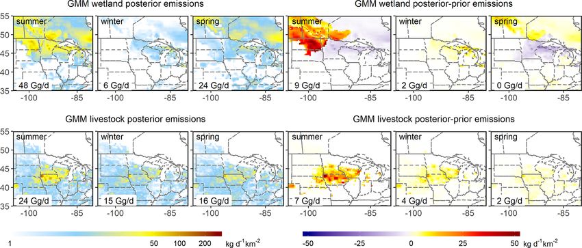
Figure 5. Wetland and livestock methane emissions derived from the GMM inversions with associated posterior–prior differences. Results
are shown for GEM1 (July–August 2017), GEM2 (January 2018) and GEM3 (May–June 2018).
Figure 6. The same as Fig. 5 but showing results for the GMM inversions with boundary condition optimization.
nure management activities; this point is discussed further in land emissions for the Upper Midwest. Below, we combine
Sect. 4. the inversion results with the individual WetCHARTs esti-
mates to derive information on key process parameters driv-
ing uncertainty in the predicted fluxes.
4 Key uncertainties for regional wetland and livestock The WetCHARTs extended ensemble includes 18 mem-
emissions bers that estimate wetland emissions F (t, d) at time t and
location d as follows:
4.1 Wetland methane fluxes: role of wetland extent and T (t,d)
emission temperature dependence F (t, d) = sA (t, d) R (t, d) q1010 . (2)
As shown above, the GEM inversions reveal spatial and tem- Here, A (t, d) is wetland extent (m2 wetland area/m2 sur-
poral errors in the WetCHARTs (ensemble mean) prior wet- face area) based on either GLOBCOVER (Bontemps et al.,
https://doi.org/10.5194/acp-21-951-2021 Atmos. Chem. Phys., 21, 951–971, 2021962 X. Yu et al.: Aircraft-based inversions quantify the importance of wetlands
Figure 7. Methane emissions derived from the adjoint 4D-Var inversions with associated posterior–prior differences. Results are shown for
GEM1 (July–August 2017), GEM2 (January 2018) and GEM3 (May–June 2018). GMM-ADJ results are similar (Figs. S7–S8).
2011) or the Global Lakes and Wetlands Database (GLWD) strated on a global basis in the WETCHIMP model
(Lehner and Döll, 2004), with temporal variability prescribed intercomparison, which reported annual flux estimates
using satellite-based surface water or reanalysis-based pre- varying by ±40 % from the mean with extensive spa-
cipitation datasets (Bloom et al., 2017); R (t, d) is het- tiotemporal disparities (Melton et al., 2013).
erotrophic respiration rate (mgC/d/m2 of wetland area) taken
as the median monthly value from the Carbon Data Model 2. Temperature dependence (q10 ). We find for both GLWD
Framework (CARDAMOM; Bloom et al., 2016); T is sur- and GLOBCOVER that a CH4 : C q10 of 3 yields the
face skin temperature (◦ C); q10 quantifies the T dependence lowest centered root-mean-square error (RMSE) com-
of methane emissions relative to heterotrophic C respiration pared to the optimized fluxes. This corresponds to an
(i.e. the CH4 : C temperature dependence), with q10 = 1, 2, average CH4 : T q10 (i.e., net T -dependence for methane
or 3; and s is a scaling factor imposing a global flux of 124.5, emissions) of 5 across the Upper Midwest domain
166, or 207.5 Tg CH4 /yr (Saunois et al., 2016; Bloom et al., (Fig. S5) versus the prior value of 2.4. Eddy covari-
2017). ance measurements at the Bog Lake peatland site in
Figure 8 shows the agreement between each of the northern Minnesota (see Fig. 1) during 2015–2017 im-
WetCHARTs ensemble members and the optimized wetland ply a CH4 : T q10 of 2.9 but based on 10 cm soil temper-
fluxes (multi-inversion average) in a Taylor Diagram. It is atures (Deventer et al., 2019). For comparison, Sheng et
apparent from Fig. 8 that (1) wetland extent and (2) CH4 : C al. (2018b) found that WetCHARTs ensemble members
emission temperature dependence (q10 ) are major factors employing CH4 : C q10 = 1 exhibited the closest agree-
controlling prediction accuracy, as discussed further below. ment with observations for wetlands in the US South-
east.
1. Wetland extent. We see from Fig. 8 that the GLWD-
based models overestimate the actual wetland emis- However, the bottom-up approach of prescribing q10
sions derived here. However, they also exhibit higher values has inherent limitations, and greater accuracy
spatial correlation with the optimized fluxes than the will require more explicit treatment of underlying
GLOBCOVER-based models do. Despite their associ- drivers. Methane in wetlands is generated through
ated overestimate (also found over the US Southeast; anaerobic microbial metabolism in waterlogged soil,
Sheng et al., 2018b), GLWD thus more accurately rep- but a separate population of methanotrophic bacteria
resents the wetland spatial distribution across the Up- above the anoxic–oxic boundary can oxidize 50 % or
per Midwest landscape. The GLWD employs maxi- more of that methane before it is able to escape to
mum wetland extent estimates derived from a range the atmosphere (Segarra et al., 2015). These competing
of sources published during 1992–2000 (DMA, 1992; processes at different depths lead to large uncertainties
UNEP-WCMC, 1993; Lehner and Döll, 2004), while when defining a single q10 value – even for an individual
the GLOBCOVER data employs year 2009 space- site. For example, long-term measurements at the Bog
based measurements from Envisat’s Medium Resolu- Lake peatland site referenced above reveal large year-
tion Imaging Spectrometer (Bontemps et al., 2011). to-year CH4 : T variability associated with water table
However, the mean 2.6-fold difference between the fluctuations (Feng et al., 2020). Previous site-level stud-
GLWD- and GLOBCOVER-based methane emissions ies likewise report a wide range of CH4 : T q10 values
for the Upper Midwest is much greater than any wet- (2–12) depending on location, year and soil temperature
land area changes during 2000–2009 (USF&WS Na- depth (Kim et al., 1998; Jackowicz-Korczyński et al.,
tional Wetlands Inventory, 2019). This high sensitivity 2010; Mikhaylov et al., 2015; Marushchak et al., 2016;
of emissions to wetland extent was likewise demon- Rinne et al., 2018).
Atmos. Chem. Phys., 21, 951–971, 2021 https://doi.org/10.5194/acp-21-951-2021X. Yu et al.: Aircraft-based inversions quantify the importance of wetlands 963
Figure 8. Taylor diagram evaluating the performance of Upper Midwest wetland emission estimates from the WetCHARTs inventory against
the optimized fluxes derived here. The colored symbols show the 18 WetCHARTs extended ensemble members, which feature three tempera-
ture sensitivity factors (CH4 : C q10 = 1, 2, or 3); three scale factors to obtain global emissions of 124.5, 166, or 207.5 Tg/yr; and two wetland
extent datasets (GLOBCOVER and GLWD, marked with open symbols and crosses, respectively). Symbols are colored by flux magnitude
relative to the optimized emissions. Three statistics are shown in these plots: (1) the slope between each symbol and the origin reflects the
spatial correlation between that model and the optimized emissions; (2) the distance between each symbol and the origin reflects the standard
deviation of that model estimate; and (3) the distance between each symbol and the optimized value reflects the centered root-mean-square
error of that model estimate relative to the optimized solution. Optimized results correspond to the multi-inversion ensemble mean.
Finally, as discussed earlier, the GEM inversions indicate a ties in the Dakotas, Wisconsin and central Minnesota, and
bottom-up wetland flux overestimate during spring that may Iowa and southern Minnesota, respectively. They also em-
reflect incorrect seasonal timing for the onset of emissions. ploy different manure management strategies: in our study
The Bog Lake peatland eddy covariance measurements sup- region, liquid systems, which have > 8× higher methane
port this idea, showing that in many years emissions rise later conversion factors than dry systems (US Environmental Pro-
in the spring than is predicted by the WetCHARTs ensem- tection Agency, 2016), account for an estimated 1 %, 57 %
ble mean (Fig. S6). Soil temperatures at depths relevant to and 95 % of beef, dairy and hog management activities, re-
microbial processes can exhibit a significant lag relative to spectively. Dry systems make up the remainder. As a result,
the surface skin temperatures used by WetCHARTs for emis- enteric emissions are thought to account for more than 95 %
sion estimation (Pickett-Heaps et al., 2011), and we hypoth- of the methane flux from beef facilities but only 60 % for
esize that this lag is the primary reason for the springtime dairies (they are minor for hog facilities) (Yu et al., 2020).
discrepancy found here. Such lags vary with environmental The above spatial segregation affords an opportunity to
conditions such as snow cover, water table, and other factors better understand methane emissions by livestock type and
(Pickett-Heaps et al., 2011). Better characterization of the (by extension) enteric versus manure contributions. To that
coupled effects of soil temperature and hydrology on emis- end, we partition our optimized fluxes by computing mean
sions is thus needed to improve the fidelity of methane flux livestock emission scaling factors (SFs) separately for model
estimates. grid cells with beef cattle, dairy cattle or hogs representing
≥ 70 % of the total animal population. Results are shown
4.2 Livestock methane: enteric emissions in Table 1 and reflect statistical averages over 2374 (beef),
well-represented but large uncertainties for manure 260 (dairy) and 1554 (hog) model grids. In each case we
present base-case estimates and uncertainties based on the
The GEM inversions point to mean underestimates in the multi-inversion mean and range, respectively.
prior GEPA livestock emissions of 24 (5–41) %, 25 (9–40) % We find in this way that beef emissions are well-
and 7 (1–15) % in summer, winter and spring, respectively. represented in the bottom-up inventory across seasons (base-
Below, we explore these discrepancies by partitioning the de- case adjustments < 15 %; Table 1). On the other hand, the
rived livestock emissions according to the geographic distri- bottom-up dairy cattle and hog emissions exhibit seasonally
bution of beef cattle, dairy cattle and hogs. dependent errors, with a base-case underestimate of ∼ 30 %
Figure 9 shows county-level animal distributions from the in summer and winter but no apparent bias in spring. Taken
2017 US Department of Agriculture Census of Agriculture together, these findings suggest an accurate treatment of en-
(USDA-NASS, 2018). Beef cattle, dairy cattle, and hogs have
distinct spatial distributions, with highest population densi-
https://doi.org/10.5194/acp-21-951-2021 Atmos. Chem. Phys., 21, 951–971, 2021You can also read