Evaluation of the coupled high-resolution atmospheric chemistry model system MECO(n) using in situ and MAX-DOAS NO2 measurements
←
→
Page content transcription
If your browser does not render page correctly, please read the page content below
Atmos. Meas. Tech., 14, 5241–5269, 2021
https://doi.org/10.5194/amt-14-5241-2021
© Author(s) 2021. This work is distributed under
the Creative Commons Attribution 4.0 License.

Evaluation of the coupled high-resolution atmospheric chemistry
model system MECO(n) using in situ and MAX-DOAS NO2
measurements
Vinod Kumar1 , Julia Remmers1 , Steffen Beirle1 , Joachim Fallmann2 , Astrid Kerkweg3 , Jos Lelieveld1 ,
Mariano Mertens4 , Andrea Pozzer1 , Benedikt Steil1 , Marc Barra5 , Holger Tost5 , and Thomas Wagner1
1 Max   Planck Institute for Chemistry, Mainz, Germany
2 Institute of Meteorology and Climate Research, Karlsruhe Institute of Technology, Karlsruhe, Germany
3 Institute of Energy and Climate Research 8, Troposphere, Forschungszentrum Jülich, Jülich, Germany
4 Deutsches Zentrum für Luft- und Raumfahrt, Institut für Physik der Atmosphäre, Oberpfaffenhofen, Germany
5 Institute of Atmospheric Physics, Johannes Gutenberg University Mainz, Mainz, Germany

Correspondence: Vinod Kumar (vinod.kumar@mpic.de)

Received: 1 February 2021 – Discussion started: 11 February 2021
Revised: 8 June 2021 – Accepted: 20 June 2021 – Published: 30 July 2021

Abstract. We present high spatial resolution (up to 2.2 ×        MAX-DOAS measurements while comparing the measured
2.2 km2 ) simulations focussed over south-west Germany us-       and simulated dSCDs. The effects of clouds on the agree-
ing the online coupled regional atmospheric chemistry model      ment between MAX-DOAS measurements and simulations
system MECO(n) (MESSy-fied ECHAM and COSMO mod-                  have also been investigated. For low elevation angles (≤ 8◦ ),
els nested n times). Numerical simulation of nitrogen diox-      small biases in the range of −14 % to +7 % and Pearson cor-
ide (NO2 ) surface volume mixing ratios (VMRs) are com-          relation coefficients in the range of 0.5 to 0.8 were achieved
pared to in situ measurements from a network with 193 lo-        for different azimuth directions in the cloud-free cases, in-
cations including background, traffic-adjacent and industrial    dicating good model performance in the layers close to the
stations to investigate the model’s performance in simulat-      surface. Accounting for diurnal and daily variability in the
ing the spatial and temporal variability of short-lived chem-    monthly-resolved anthropogenic emissions was found to be
ical species. We show that the use of a high-resolution and      crucial for the accurate representation of time series of mea-
up-to-date emission inventory is crucial for reproducing the     sured NO2 VMR and dSCDs and is particularly critical when
spatial variability and resulted in good agreement with the      vertical mixing is suppressed, and the atmospheric lifetime of
measured VMRs at the background and industrial locations         NO2 is relatively long.
with an overall bias of less than 10 %. We introduce a compu-
tationally efficient approach that simulates diurnal and daily
variability in monthly-resolved anthropogenic emissions to
resolve the temporal variability of NO2 .                        1   Introduction
   MAX-DOAS (Multiple AXis Differential Optical Ab-
sorption Spectroscopy) measurements performed at Mainz           Regional atmospheric chemistry and transport models are
(49.99◦ N, 8.23◦ E) were used to evaluate the simulated tro-     important for the study and forecasting of atmospheric pro-
pospheric vertical column densities (VCDs) of NO2 . We pro-      cesses at fine spatial resolutions. The high spatial resolu-
pose a consistent and robust approach to evaluate the verti-     tion of these models allows us to resolve localized emis-
cal distribution of NO2 in the boundary layer by comparing       sions (e.g. industrial and urban clusters) and quantify their
the individual differential slant column densities (dSCDs)       impacts on non-linear photochemical processes, e.g. ozone
at various elevation angles. This approach considers details     production (Vinken et al., 2014; Visser et al., 2019; Mertens
of the spatial heterogeneity and sensitivity volume of the       et al., 2020a) as well as on heterogeneous processes, e.g. par-

Published by Copernicus Publications on behalf of the European Geosciences Union.
5242                                                          V. Kumar et al.: Regional model evaluation using MAX-DOAS

ticulate nitrate production (Chen et al., 2020). Various stud-     computationally inefficient due to the high readout time and
ies have shown that significant improvements in satellite re-      subsequent requirement for interpolation on the model grid.
trievals can be achieved through the incorporation of highly          The evaluation of high-resolution mesoscale models is
resolved a priori trace gas and aerosol fields calculated by       even more challenging due to the limited availability (in situ
high-resolution regional models (Valin et al., 2011; Liu et al.,   measurements) and unavailability (e.g. satellite observations)
2020; Ialongo et al., 2020).                                       of reference datasets. TROPOMI (TROPOspheric Monitor-
   Regional models achieve high resolution by employ-              ing Instrument) aboard the Sentinel-5P satellite (Veefkind
ing nesting around the location of interest, in which a            et al., 2012) has a high spatial resolution (up to 3.5×5.5 km2 )
fine-resolution model domain receives meteorological and           and is in principle well suited for comparison of the tropo-
chemical boundary conditions from a coarser resolution             spheric vertical column densities (VCDs) simulated by the
model spanning a broader area. The MECO(n) (MESSy-                 model. However, the limited temporal information – gener-
fied ECHAM and COSMO models nested n times) regional               ally measurements from one overpass per day – precludes an
model system developed by Kerkweg and Jöckel (2012b)               evaluation of diurnal profiles; hence, TROPOMI is not well
allows for online coupling between different nests and in          suited to demonstrating the advantages of considering diur-
this way facilitates frequent updates of meteorological and        nally varying input emissions. Besides VCDs, conventional
chemical boundary conditions. The use of MESSy submod-             model evaluation studies are often restricted to the evaluation
els for this coupled system also ensures consistent treatment      of concentrations at discrete layers (most often at the surface)
of chemical speciation, chemistry and several other relevant       using in situ measurements which are limited with respect
processes governing the concentration of chemical species          to the temporal and spatial coverage. Evaluations of model
among various nests. A chemical evaluation of MECO(n)              vertical profiles are even rarer due to the paucity of ver-
over Europe was performed by Mertens et al. (2016) for a           tically resolved measurements (e.g. balloon-based and air-
set-up at ∼ 12 × 12 km2 spatial resolution for nitrogen diox-      craft measurements), which are technically very challenging.
ide (NO2 ), ozone (O3 ) and carbon monoxide (CO). The              For example, discrepancies between regional models (WRF-
main strength of MECO(n), i.e. the online coupling with the        Chem and CHIMERE) and measurements were proposed to
COSMO model, makes it suitable for performing very high            arise due to inappropriate parametrization of the turbulent
resolution (e.g. < 3 × 3 km2 ) simulations. For example, the       diffusion constant; however, this could not be verified due
operational COSMO model is already being used for weather          to the lack of vertically resolved NO2 measurements (Kuik
forecasts at a spatial resolution of 2.8 × 2.8 km2 by the Ger-     et al., 2018; Schaap et al., 2015). Mertens et al. (2016) evalu-
man Meteorological Service (Deutscher Wetterdienst) and at         ated the vertical profiles of O3 simulated by MECO(n) using
1 × 1 km2 by the Federal Office of Meteorology and Clima-          ozone-sonde data, but this provides little information about
tology, Switzerland (MeteoSwiss). Similar high-resolution          the variability within the boundary layer which is masked by
model simulations including chemistry have been shown to           that in the upper troposphere (above 400 hPa or ≈ 7 km).
better represent local maxima (e.g. isolated point sources,           In this regard, MAX-DOAS (Multiple AXis Differen-
road networks and ship tracks) and facilitate understanding        tial Optical Absorption Spectroscopy) measurements (Hön-
of sector-specific impacts on secondary pollution (e.g. ozone      ninger et al., 2004) provide a unique opportunity for model
production) (Colette et al., 2014; Mertens et al., 2020a).         evaluation for a larger representative area (a few square kilo-
However, comparison with in situ measurements showed that          metres) and over long temporal scales. To our knowledge, re-
these gains could only be quantitatively determined up to          gional model comparison studies with MAX-DOAS are very
a resolution of ∼ 7 × 7 km2 , beyond which major improve-          limited (e.g. Shaiganfar et al., 2015; Vlemmix et al., 2015;
ments were not observed (Colette et al., 2014). In most of         Blechschmidt et al., 2020) and mostly focus on the tropo-
the cases, the improvement was limited by the resolution of        spheric VCDs. These studies have shown moderate correla-
the input emission inventory used in these studies, which          tions between MAX-DOAS and regional model calculated
are available at a much coarser resolution than that of the        VCDs with major differences arising due to inappropriate
model set-up. Apart from the coarse resolution, further limi-      representation of anthropogenic emissions, differences be-
tations in such comparisons are imposed by the availability of     tween model-simulated and actual wind vectors, the pres-
mostly outdated anthropogenic emissions inventory and lim-         ence of clouds, and uncertainties related to the MAX-DOAS
ited information about short-term temporal variability (e.g.       VCD retrieval. Further limitations in these comparisons arise
day of the week or hour of the day) (Kuik et al., 2018). In        due to assumptions of horizontal homogeneity and the chal-
most cases, input emission inventories are available at tem-       lenges associated with accurately defining the area/volume
poral resolutions of months to years, but in reality, emissions    for which the MAX-DOAS measurements are sensitive. In
from several sectors (e.g. road transport, residential combus-     addition to the VCDs, there is additional information content
tion) vary markedly depending on the hour of the day and           in the MAX-DOAS measurements (e.g. spatial distribution
day of the week. From a modelling perspective, however, in-        of trace gases), which comes from scans performed at differ-
corporating high temporal resolution input emissions can be        ent elevation angles, thus probing the atmosphere along dif-
                                                                   ferent light paths. This information can be utilized to evaluate

Atmos. Meas. Tech., 14, 5241–5269, 2021                                             https://doi.org/10.5194/amt-14-5241-2021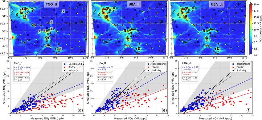
V. Kumar et al.: Regional model evaluation using MAX-DOAS                                                                 5243

the performance of regional models in accurately simulating      as CM50 hereafter), the second one at 0.0625◦ × 0.0625◦
the spatial distribution within the boundary layer.              (∼ 7 × 7 km2 ; referred to as CM07 hereafter) and the third
   In this paper, we present high-resolution (up to 2.2 ×        one at 0.02◦ × 0.02◦ (∼ 2.2 × 2.2 km2 ; referred to as CM02
2.2 km2 ) MECO(3) simulations of NO2 over south-west Ger-        hereafter). All three COSMO/MESSy domains are set up in
many using a high spatial resolution and up-to-date input        a rotated coordinate system with the location of the north
emission inventory. We also effectively account for the day-     pole at 40◦ N and −170◦ E. The CM07 domain is focussed
of-the-week and diurnal variability in anthropogenic emis-       around Germany, and CM02 further zooms in to south-west
sions in the model simulations by applying sector-specific       Germany, as shown in Fig. 1. CM50 and CM07 have 40
hourly scaling factors to the monthly-resolved anthropogenic     terrain-following vertical levels extending up to 22.7 km,
emissions. The model description, details of MAX-DOAS            while CM02 has 50 terrain-following vertical levels extend-
measurements and analyses as well as other reference data        ing up to 22 km. In all the three domains, the lowermost at-
are provided in Sect. 2. We evaluate the model performance       mospheric model layer has a thickness of 20 m, while the
with respect to two input emission inventories and tempo-        lowest 1 km is split into 11 levels for CM50 and CM07 and
ral resolution of emissions through comparison with in situ      12 levels for CM02. The thickness of the vertical layers in-
measurements in Sect. 3.2 and MAX-DOAS tropospheric              creases with altitude. The time steps for CM50, CM07 and
NO2 VCDs in Sect. 3.3. The TROPOMI comparison will be            CM02 are 120, 60 and 20 s, respectively. The online cou-
the focus of a future study. In this paper, we introduce a so-   pling enables the specification of boundary conditions at each
phisticated and consistent approach for MAX-DOAS com-            time step by the respective driving model and is particularly
parison, which overcomes the limitations of previous such        advantageous for complex atmospheric chemistry modelling
comparisons. We also evaluate the performance of the model       involving hundreds of chemical tracers. Convection is param-
in reproducing the vertical distribution of NO2 within the       eterized according to the Tiedtke–Bechtold scheme for both
boundary layer.                                                  CM50 and CM07 domains, while for the CM02 domain only
                                                                 shallow convection is parameterized according to the Tiedtke
                                                                 scheme (Bechtold et al., 2001; Tiedtke, 1989).
2     Methods                                                       The MECO(n) model set-up achieves a very high consis-
                                                                 tency within the model chain, as all four model instances
2.1    Model description                                         (EMAC and three times COSMO/MESSy) use MESSy and
                                                                 thus imply the very same chemical speciation and process
We use the one-way coupled model system MECO(3)                  formulations for the chemical processes (e.g. online/offline
(Kerkweg and Jöckel, 2012a, b) based on MESSy ver-               emission of chemical tracers, ONEMIS/OFFEMIS; chem-
sion 2.54 (Jöckel et al., 2010), which couples the global        istry, MECCA; dry deposition, DDEP; wet scavenging,
chemistry climate model EMAC (Jöckel et al., 2006) one-          SCAV and photolysis, JVAL) (Jöckel et al., 2010; Tost et al.,
way to the regional model COSMO-CLM/MESSy (called                2006; Kerkweg et al., 2006a; Sander et al., 2014; Kerkweg
COSMO/MESSy hereafter). COSMO-CLM is the commu-                  et al., 2006b). Since deep convection is resolved in the CM02
nity model of the German regional climate research com-          domain, the MESSy submodel CVTRANS (Tost et al., 2010)
munity jointly further developed by the CLM-Community            used to calculate the tracer transport due to convection is not
(Rockel et al., 2008). The core driving model for EMAC           used in this domain. Consequently, convective scavenging
is ECHAM5 version 5.3.02 (Roeckner et al., 2003), and for        and convective rain flux are also disabled in the CM02 do-
COSMO/MESSy it is COSMO 5.00_clm10 (Rockel et al.,               main when using the SCAV submodel (Tost et al., 2006). For
2008; Steppeler et al., 2003). EMAC is configured with           the chemical mechanism in MECCA, we use the Mainz Iso-
T106L31ECMWF spectral resolution corresponding to a              prene Mechanism (MIM 1) (Pöschl et al., 2000), including
grid resolution of ∼ 1.1◦ × ∼ 1.1◦ , extending up to 10 hPa      142 gaseous chemical species involved in 236 gas and multi-
(≈ 30 km over Europe) vertically in 31 vertical layers and       phase reactions and 74 photochemical reactions.
time step of 360 s. The global model meteorology (tempera-          For the global model and the CM50 domain, EDGAR
ture, vorticity, surface pressure and divergence) is nudged to   4.3.2 anthropogenic emissions (0.1◦ ×0.1◦ globally) (Crippa
6-hourly ECMWF ERA-Interim reanalysis data. Model sim-           et al., 2018) have been used, while for the CM07 and
ulations are performed for May 2018, i.e. from 1 May 2018        CM02 domain two different anthropogenic emission scenar-
00:00:00 until 1 June 2018 00:00:00. The initial chemical        ios, namely TNO MACC III (Kuenen et al., 2014) (avail-
conditions for the regional model instances are provided by      able for Europe until 2011) and UBA (Strogies et al., 2020)
an EMAC simulation starting 3 years before the MECO(n)           (Umweltbundesamt; available for Germany, until 2018), have
simulations start, i.e. on 1 March 2015.                         been employed. Total annual anthropogenic emissions of
   The three instances of the COSMO/MESSy model are              NOx within Germany are 366 and 288 Gg(N) for UBA (for
coupled online one-way from coarser resolution to finer res-     2018) and TNO MACC III (for 2011), respectively. To put
olution. The first instance of COSMO/MESSy has a spa-            these estimates in perspective, EDGAR v5.0 (Crippa et al.,
tial resolution of 0.44◦ × 0.44◦ (∼ 50 × 50 km2 ; referred to    2020) annual anthropogenic NOx emissions for 2011 and

https://doi.org/10.5194/amt-14-5241-2021                                          Atmos. Meas. Tech., 14, 5241–5269, 2021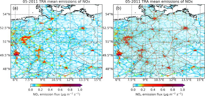
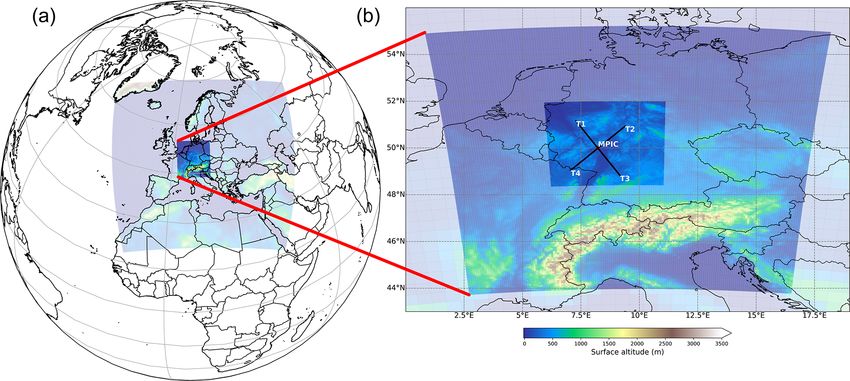
5244                                                            V. Kumar et al.: Regional model evaluation using MAX-DOAS

Figure 1. MECO(3) domains in panel (a) colour-coded according to the surface altitude. A close-up of the map in the right panel shows the
CM07 and CM02 domains. The location of MPIC (Max Planck Institute for Chemistry) is shown as the red dot in panel (b) with the arrows
pointing in the viewing direction of the four telescopes.

2015 for Germany are 389.2 and 366.9 Gg(N). The spa-                   model time step is calculated by interpolating the time series
tial resolution of TNO MACC III and UBA emissions are                  and applying it to the monthly emissions; subsequently, the
0.0625◦ (latitude) ×0.125◦ (longitude) and 1 km × 1 km, re-            emissions flux and tendency (change in volume mixing ratio
spectively. For the TNO MACC III and UBA emissions, NOx                (VMR) per model time step) are calculated using the ONE-
was originally expressed as kg yr−1 and kt yr−1 , respectively,        MIS submodel (Kerkweg et al., 2006b). The MESSy OF-
of NO2 , which were further converted as molecules m−2 s−1             FEMIS submodel (Kerkweg et al., 2006b) updates the ten-
for use in model simulations. In Appendix A and Fig. A3, we            dencies for emissions from the sectors for which a finer tem-
also compare the contribution of individual sectors towards            poral profile is not necessary (e.g. agriculture, waste manage-
the total anthropogenic NOx emissions in the TNO MACC                  ment, refineries).
III and UBA inventory.                                                    The anthropogenic emissions are vertically distributed de-
   Three MECO(3) simulations were performed with differ-               pending on the source sectors according to the recommen-
ing fine temporal variation for the TNO MACC III and UBA               dation by Pozzer et al. (2009) except that the lowest injec-
anthropogenic emissions, as summarized in Table 1.                     tion height is reduced to 10 m as opposed to 45 m. This was
   The subscript “di” in Table 1 indicates the use of the              necessary because the lowest level of COSMO extends from
diurnal and day-of-the-week variability in NOx and CO                  the surface to 20 m altitude, while the median lowest level
emissions from the road transport and residential and non-             height of EMAC (as used by Pozzer et al., 2009) is about
industrial combustion sectors (see Appendix A for further              60 m. Lightning NOx is calculated for the global model ac-
details). Similarly, the subscript “fl” (e.g. in the TNOfl and         cording to the parameterizations by Grewe (2009) and trans-
UBAfl set-ups) indicates that constant anthropogenic emis-             ferred to the subsequent instances of COSMO using the
sions (and a flat diurnal pattern) are used for the com-               Multi-Model-Driver (MMD) coupling of the MMD2WAY
plete month. The sector-wise anthropogenic emissions are               submodel (Kerkweg et al., 2018). The lightning frequency
imported via the IMPORT submodel (Kerkweg and Jöckel,                  was scaled to produce 2.5 Tg(N) yr−1 globally. Soil NOx
2015). For specifying the temporal profiles (diurnal and day           and biogenic emissions (e.g. isoprene and monoterpenes)
of the week) in the anthropogenic emissions, we first created          are calculated online using the ONEMIS submodel sepa-
hourly-resolved time series of scaling factors to be applied to        rately in EMAC and individual COSMO/MESSy instances.
the monthly-mean values using the factors shown in Fig. A1.            For May 2018, soil NOx emissions were calculated to be
Please note that the factors have a weekly cycle, and these            17.8 and 2.4 Gg(N) for the CM07 and CM02 domains, re-
are normalized such that the total emission over a week is             spectively. Soil NOx emission over the whole of Germany
conserved for a given sector. Individual hourly time series            in the CM07 domain was 5.9 Gg(N) for May 2018. The soil
of emission scaling factors are imported via IMPORT_TS                 NOx emission calculated online is smaller as compared to the
(Kerkweg and Jöckel, 2015). The scaling factor for a specific          estimated 19.0 Gg(N) for May 2015 from agricultural soils

Atmos. Meas. Tech., 14, 5241–5269, 2021                                                  https://doi.org/10.5194/amt-14-5241-2021

V. Kumar et al.: Regional model evaluation using MAX-DOAS                                                                   5245

Table 1. Model set-ups.

            Simulation ID   Anthropogenic emissions (in CM07 and CM02 domains)         Temporal resolution of emissions
            TNOfl           TNO MACC III                                               Monthly
            UBAfl           UBA (for Germany) and TNO MACC III (outside Germany)       Monthly
            UBAdi           UBA (for Germany) and TNO MACC III (outside Germany)       Hourly

and manure management sectors combined by EDGAR v5.0               elevation angle. Since MECO(3) was configured to write the
(Crippa et al., 2020). Non-methane volatile organic com-           output for the CM02 domain at an hourly frequency as mean
pound (NMVOC) emissions were also provided as lumped               values, we also average the MAX-DOAS retrieved quanti-
group of species, which were speciated according to the rec-       ties (see Sect. 2.2.2) at a similar frequency while discarding
ommendation by Huang et al. (2017).                                retrieval with high spectral analysis rms values.

2.2   Four-azimuth MAX-DOAS measurements                           2.2.1   Cloud classification

                                                                   A cloud classification was performed using MAX-DOAS
Multiple AXis Differential Optical Absorption Spectroscopy         measurements of the colour index (CI; the ratio of measured
(MAX-DOAS) measurements were performed using a                     signal at 330 and 390 nm) and the O4 dSCDs according to the
custom-built instrument installed at the rooftop of the Max        method described by Wagner et al. (2016). In order to gener-
Planck Institute for Chemistry (MPIC) building (49.99◦ N,          ate robust thresholds for the cloud classification, 1 month of
8.23◦ E; 150 m a.m.s.l.; the red dot in Fig. 1). The instrument    data are not sufficient; hence, we used a longer time series of
consists of four telescopes (T1, T2, T3 and T4 pointing at az-     MAX-DOAS measurements from 27 March until 14 Septem-
imuth angles of 321, 51, 141 and 231◦ , respectively, clock-       ber 2018. We performed cloud classification separately using
wise from the north). The intersecting arrows in Fig. 1 in-        measurements performed by the four telescopes. Figure C1
dicate the azimuth direction of the four telescopes. Individ-      summarizes the cloud conditions for all the days of May 2018
ual optical fibre bundles transmit the light from the respec-      for telescope T2. Briefly, clear-sky conditions were observed
tive telescopes to a temperature-controlled spectrograph. The      from 5 May 2018 until the afternoon of 9 May 2018. On other
spectrograph consists of a 2D (1023 × 255) CCD (charge-            days, cloudy conditions were observed for several hours with
coupled device) detector array. The incoming light of the          sky conditions alternating between broken clouds, continu-
four telescopes is projected to different row regimes of the       ous clouds and optically thick clouds. The cloud classifica-
CCD. This set-up reduces the instrumental differences be-          tion results for the other telescopes were similar to those of
tween the measurements to a minimum. The measurements              T2.
are performed along the four viewing directions simultane-
ously such that all the telescopes (T1–T4) point towards the       2.2.2   Retrieval of differential box air mass factors
same elevation angle (EA). One complete measurement se-                    using 3D aerosol profile inversion
quence for each telescope involved measurements at eight
off-axis elevation angles (1, 2, 3, 5, 8, 10, 15 and 30◦ ) and     As mentioned above, the dSCDs retrieved from MAX-DOAS
in the direction of the zenith. The field of view at 1◦ eleva-     measurements depend on the differential light path between
tion angle was blocked partially for the different telescopes      the off-axis (EA = α) and zenith measurements. dSCDs are
and hence was discarded from the subsequent analyses. We           related to the VCDs via the differential air mass factors
applied the DOAS principle (Platt and Stutz, 2008) to the          (dAMFs) according to the following equation:
measured spectra to retrieve the elevation-angle-dependent
differential slant column densities (dSCDs) of NO2 and the                  dSCDα
oxygen dimer (O2 −O2 or O4 ), adapting to the fit setting de-      VCD =          .                                           (1)
                                                                            dAMFα
scribed in Table C1. The dSCDs can be regarded as the dif-
ference between the concentration integrated along the light       The O4 mixing ratio is almost constant throughout the tro-
path at a chosen elevation angle and the concentration in-         posphere, and its VCD only depends on the atmospheric
tegrated along the direction of the zenith. This approach is       temperature and pressure profile. Hence, using measured O4
used to eliminate the stratospheric information and retrieve       dSCDs and the knowledge of O4 VCDs, the corresponding
the tropospheric contribution.                                     dAMFs can be calculated. If we visualize the atmosphere in
   In order to retain only the highest quality DOAS fit results,   several discrete layers, the partial dSCD in a specific layer
we discarded all retrievals with fit rms (root mean square)        (k) would be related to the partial VCD (Vk ), and the dif-
values greater than 1.0×10⁻³ . NO2 VCDs are retrieved using        ferential box air mass factor (dbAMFα,k ) would be specific
the geometric approximation on the measured dSCDs at 30◦           for the layer k in a similar way as in Eq. (1). dAMF can be

https://doi.org/10.5194/amt-14-5241-2021                                            Atmos. Meas. Tech., 14, 5241–5269, 2021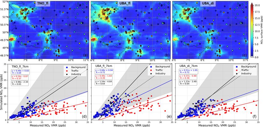
5246                                                          V. Kumar et al.: Regional model evaluation using MAX-DOAS

reconstructed from the dbAMFα,k according to Eq. (2):              man Meteorological Service (Deutscher Wetterdienst) for
           P                                                       meteorological evaluation in the CM02 set-up (DWD, 2019).
               Vk × dbAMFα,k
dAMFα = k P                  .                        (2)          Hourly measurements of surface temperature, relative hu-
                    k Vk                                           midity and wind speed are available for 620, 501 and 283
   The presence of aerosols can change the light path and          stations, respectively, in Germany for May 2018; out of these,
hence the dSCDs (and consequently the dAMFs). Profile in-          178, 197 and 95, respectively, fall within the CM02 domain.
version algorithms can find the optimal aerosol extinction            In situ measurements of NO2 and O3 are available from the
profiles corresponding to the measured O4 dSCDs for a se-          German Environment Agency (Umweltbundesamt) (Minkos
quence of elevation angles (Wagner et al., 2004; Clémer            et al., 2019) from 410 and 266 stations, respectively, across
et al., 2010; Wagner et al., 2011). This can be subsequently       Germany for May 2018. Among the 410 NO2 measurement
used to calculate the dbAMFα,k in the discrete atmospheric         stations, 193 fall within the CM02 domain, out of which
layer indexed by k. In addition to the O4 VCDs and mea-            119, 60 and 14 stations represent background, traffic and
sured dSCDs, the profile inversion algorithms require an of-       industrial locations, respectively. For O3 , 120 stations are
fline look-up table of O4 dAMFs corresponding to various           within the CM02 domain, out of which 109, 3 and 8 sta-
combinations of measurement geometry and aerosol extinc-           tions represent the background, traffic and industrial loca-
tion profiles calculated using radiative transfer models (e.g.     tions, respectively. For most of the stations within the CM02
McArtim; Deutschmann et al., 2011).                                domain, NO2 is measured online using the chemilumines-
   We used the profile inversion algorithm π -MAX (Param-          cence method, in which NO2 is reduced to NO using a heated
eterized profile Inversion for MAX-DOAS measurements)              molybdenum converter prior to its detection (Eickelpasch
(Remmers, 2021) for the retrieval of the dbAMFs. In com-           and Eickelpasch, 2004). Only at Schmücke (DEUB029), a
parison to the traditional parameterized profile inversion al-     photolytic converter is used in place of the molybdenum
gorithms (e.g. MAPA; Beirle et al., 2019), which only param-       converter, whereas at Pfälzerwald-Hortenkopf (DERP017), a
eterizes the aerosol optical depth (AOD) and vertical profiles     CAPS (Cavity Attenuated Phase Shift Spectroscopy) instru-
of aerosol extinction (e.g. shape, s, and height, h, of the pro-   ment is used for measurement of NO2 (https://www.env-it.
file) for a 1D retrieval (along altitude), π -MAX includes ad-     de/stationen/public/downloadRequest.do, last access: 13 July
ditional parameters related to the horizontal gradients in the     2021). O3 is measured online using the UV absorption tech-
viewing direction.                                                 nique at all the stations. The measured in situ data are avail-
   Figure 2 shows the schematic of a traditional profile in-       able at 1 h resolution.
version for an example case of AOD = 1.0, h = 1 and vari-
ous parameterizations of s representing the respective profile
shapes as well as additional parameters g and l for π -MAX.        3     Results and discussion
These additional parameters describe the linear aerosol ex-
tinction change (g) from the telescope location to a specific      3.1    Meteorological evaluation: surface temperature,
distance (l). Hence, they allow for retrievals of 2D dbAMFs               relative humidity and wind speed
(and aerosol extinction profiles) as a function of distance
from the telescope and altitude from the instrument, if mea-       In the online coupled MECO(n) system, COSMO/MESSy
surement in only one azimuth direction is considered. If           instances are not nudged directly towards the reanalysis
measurements in several azimuth directions are combined,           dataset. Rather, these receive the meteorological boundary
3D retrievals can be performed. In the current π -MAX set-         conditions from EMAC for the first instance and from the
up, l is fixed to 10 km. The dSCD measurements in all four         antecedent COSMO/MESSy for each subsequent instance on
directions are used simultaneously with the constraint that        the four sides of the domain and the damping layer (ca. 11 km
the profile at the origin (location of the instrument) is the      for CM50 and CM07 and 10.7 km for the CM02 domain).
same for all the telescopes.                                       Hence individual COSMO/MESSy instances of MECO(n)
   The quality of the profile retrieval from π -MAX can be         can develop their own dynamics, which might result in a de-
qualified using the rms of the dSCD fit corresponding to           viation from the actual meteorology. Hofmann et al. (2012)
each complete elevation sequence. In order to retain only the      have evaluated the MECO(n) meteorology and demonstrated
highest quality profile inversion results, we have retained re-    comparable performance with respect to a similar model with
trievals corresponding to rms values less than 0.04 times the      offline coupling. Here, we briefly evaluate the performance
O4 VCDs.                                                           of MECO(n) in the CM02 set-up with respect to the mea-
                                                                   sured surface temperature, relative humidity and wind speed
2.3    In situ chemical and meteorological measurement             close to the surface.
       data                                                           The ability of the model to reproduce the temporal vari-
                                                                   ability at multiple measurement stations can be evaluated us-
We used the surface temperature, relative humidity and wind        ing Taylor diagrams (Taylor, 2001), where we show the Pear-
measurement data from the Climate Data Center of the Ger-          son correlation coefficient (R), relative root mean square dif-

Atmos. Meas. Tech., 14, 5241–5269, 2021                                             https://doi.org/10.5194/amt-14-5241-2021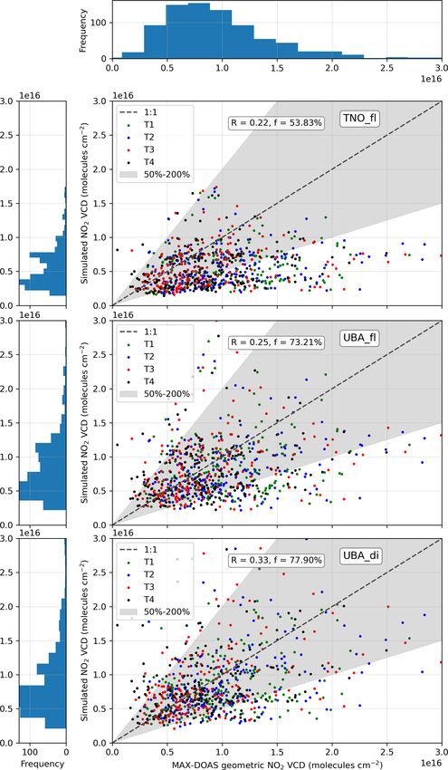
V. Kumar et al.: Regional model evaluation using MAX-DOAS                                                                              5247

Figure 2. (a) Schematic illustration of traditional 1D parameterized profile inversion which constrains AOD, height (h) and shape (s) of
the profile. The example shown here corresponds to a scenario with AOD = 1.0, h = 1.0 and four different profile shapes representing
exponential decrease, box profile, elevated box profile and linearly increasing profiles. (b) Additional parameters l and g further constrain
the horizontal gradients of AOD for 2D profile inversion. Here, g denotes a linear change in AOD for a distance l along the viewing direction
of the MAX-DOAS instrument.

ference (RMSD) and relative standard deviation (RSD) with                from the in situ measurement stations are depicted as square,
respect to the hourly resolution measured data. The Taylor               circle and pentagon markers for background, traffic-adjacent
diagrams for these parameters are shown in Fig. 3.                       and industrial sites, respectively, overlaid on the maps using
   For surface temperature, the trends in the hourly-resolved            the same colour scale as that for simulated VMRs.
time series agree quite well with Pearson correlation coef-                 Overall, the spatial distribution of NO2 VMRs is as ex-
ficients generally between 0.8 and 0.9. The spatial patterns             pected, such that the high values are observed in densely
of the surface temperatures are also represented very well               populated areas, e.g. the Ruhr area, Luxembourg, around
as inferred from small and precise RMSD values of ca. 0.5.               Frankfurt, Mannheim, Karlsruhe and Stuttgart. For the sim-
RSD values of less than 1 indicate that observed temporal                ulation with the high-resolution UBA emissions, we observe
variability in the model has a smaller amplitude than that of            many details in the NO2 surface concentration with higher
the measurements. There is a cold bias of ∼ 3 ◦ C across the             values coinciding with the major motorways of Germany
domain, which is similar to that observed by Mertens et al.              which were not so obvious with TNOfl (e.g. A61 motor-
(2016) for Germany in summer. Previous long-term evalua-                 way between Köln and Bingen, A3 between Frankfurt and
tion of the COSMO-CLM model has shown a cold bias of                     Bingen, A48 and A1 connecting Koblenz and Luxembourg,
2–2.5 ◦ C compared to observation of the annual mean sur-                and A4 and A9 between Gießen and Leipzig). The perfor-
face temperature over Germany, which increases in the sum-               mance of the model in reproducing the spatial variability can
mertime (Böhm et al., 2006). This bias is most probably due              be quantitatively described using the root mean square de-
to inaccurate representation of root depth and soil temper-              viation (RMSD) between the monthly-mean measured and
ature damping in the soil model. For relative humidity, the              simulated NO2 VMRs for all the measurement stations com-
trends in the hourly-resolved time series agree reasonably               bined. We note that using the high-resolution UBA emis-
well with Pearson correlation coefficient generally between              sions improves the RMSD for background locations from
0.5 and 0.7. Both positive and negative mean biases are ob-              3.3 ppb (∼ 45 % of the measured mean) for TNOfl to 2.7 ppb
served for the different stations. For wind speeds, the Pearson          (∼ 37 %). Since UBA emissions are up to date and are avail-
correlation coefficients are generally between 0.2 and 0.5, but          able for the same year as that of simulation, the mean bias
the bias was generally small and in the range of ±1 m s−1 .              for the background locations also improves from −2.0 ppb
                                                                         (−27 %) for TNOfl to −0.5 ppb (−7 %) for UBAfl . At loca-
3.2   Evaluation of surface mixing ratios of NO2                         tions near heavy traffic, the bias improved from −12.5 ppb
                                                                         (−63 %) for TNOfl to −10.4 ppb (−52 %) for UBAfl .
                                                                            Even though the anthropogenic NOx emissions have re-
In this section, we present the model results for simulated
                                                                         duced by ∼ 15 % over Europe from 2011 (the most recent
NO2 surface volume mixing ratios (VMR) and compare with
                                                                         year for which TNO emissions are available) to 2017 (EEA,
the in situ observations for May 2018. Figure 4 shows the
                                                                         2019), total NOx emissions over Germany are ∼ 21 % lower
spatial distribution of monthly-mean NO2 VMRs in the low-
                                                                         in TNO MACC III as compared to UBA. For the TNO
est vertical layer (0–20 m) for the CM02 domain for the three
                                                                         MACC III, NOx emissions are lower across all the sec-
model set-ups listed in Table 1. The monthly-mean VMRs

https://doi.org/10.5194/amt-14-5241-2021                                                    Atmos. Meas. Tech., 14, 5241–5269, 2021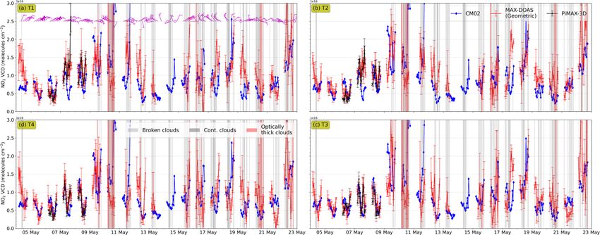
5248                                                               V. Kumar et al.: Regional model evaluation using MAX-DOAS

Figure 3. Taylor diagrams showing the agreement between measured and model-calculated surface temperatures (a) and relative humidity (b)
and wind speed (c). Each data point corresponds to an individual measurement station, with a total of 178, 197 and 95 stations for surface
temperature, relative humidity, and wind speed, respectively.

Figure 4. (a, b, c) Spatial distribution of monthly-mean NO2 surface VMRs for the three simulations using different emission inventories
(a, d: TNO, b, e: UBA without diurnal variations, c, f: UBA with diurnal variations) for CM02 for May 2018. The square, circle and
pentagon markers overlaid on the maps represent the monthly-mean measured NO2 VMRs for background, traffic and industrial locations,
respectively. The numbers on the top left panel correspond to the following German cities in decreasing order of latitude coordinate values,
i.e. 1: Duisburg, 2: Kassel, 3: Köln, 4: Gießen, 5: Koblenz, 6: Frankfurt, 7: Mainz, 8: Bingen, 9: Mannheim, 10: Karlsruhe 11: Stuttgart.
(d, e, f) Scatter plot and orthogonal distance regression weighted by the inverse of the square of the standard deviation of simulated monthly-
mean NO2 surface VMRs with respect to the in situ measured values for different station types (background: blue square; traffic: red circle,
and industrial: black pentagon).

tors except for ship transport and comparable for residential             NOx emissions (for 2018) (see Fig. A3). Recent top-down
and non-industrial combustion. For the three strongest NOx                emissions estimates over urban centres in Germany have also
emission sectors, e.g. road transport, energy industries and              pointed towards an underestimation of as much as a factor of
other industries, TNO MACC III NOx emissions (for 2011)                   2 from the transport sector and 1.5 overall (Kuik et al., 2018)
are ∼ 19 %, 34 % and 18 %, respectively, lower than the UBA               by the TNO MACC III emissions, even by considering a con-

Atmos. Meas. Tech., 14, 5241–5269, 2021                                                      https://doi.org/10.5194/amt-14-5241-2021
V. Kumar et al.: Regional model evaluation using MAX-DOAS                                                                 5249

servative approach. Top-down emission estimates using OMI         urnal profiles of emissions in the transport sector increase
(Ozone Monitoring Instrument) NO2 measurements also in-           the NOx amount to more than twice as much during the day-
dicated an underestimation of NOx emission by more than           time when the atmospheric lifetime is lower and decreases
50 % over western Germany and other parts of Europe by the        to less than one-quarter during the night when lifetime is
TNO MACC III emission inventory (Visser et al., 2019). It         high. Hence, overall, the monthly-mean surface NO2 VMR
should be noted that exclusion of soil NOx emissions from         decreases when a diurnal profile is applied to NOx emissions.
the TNO MACC III inventory also contributed towards the           The normalized standard deviation (relative to the standard
large underestimation in the estimates by Visser et al. (2019).   deviation of measured VMRs) improves by inclusion of di-
The underestimation of the a priori NOx emissions is the          urnal profiles, as we observe more stations with values in the
most important factor for the large negative bias in the TNOfl    0.5–1.5 range.
set-up. Getting up-to-date emission inventories is difficult,         Using the different COSMO/MESSy instances of the
and we could only get these data for Germany, but for future      MECO(3) system, we are able to investigate the importance
studies with simulation involving larger domains, which in-       of model resolution if the same emission inventory is used for
clude more countries, it is recommended to use more up-to-        different model resolutions. Figure C2 shows the spatial dis-
date emission inventories. The situation of underestimation       tribution of simulated NO2 surface VMRs and the agreement
of NOx emissions over Germany (and most parts of Europe)          with measurements for the CM07 set-up in a similar way as
is different from that observed in the USA, where national        Fig. 4 for CM02. We note that for TNOfl there is only very
emissions inventories are biased high by as much as 30 %–         little further detail in the spatial distribution for CM02 as
60 % (Travis et al., 2016).                                       compared to CM07. Meteorology (e.g. wind patterns) might
   Unlike for the background locations, we do not observe         be better resolved using a fine model resolution on indi-
a major improvement for the traffic-adjacent locations us-        vidual days. Still, when averaged over several days, these
ing the UBA emissions. Even at such high spatial resolution       will be smoothed, and the spatial patterns would be limited
(2.2 × 2.2 km2 ), the spatial smoothing leads to insufficient     by the resolution of the input emissions inventory. Conse-
reproduction of peaks for locations close to strong emission      quently, we also did not observe any significant improvement
sources as also documented by Shaiganfar et al. (2015). An-       in the RMSD (45 %) between the monthly-mean measured
other factor which could contribute to the differences be-        and simulated NO2 VMRs as compared to the CM07 simu-
tween measured and simulated NO2 is related to the chemi-         lation (RMSD = 48 %) using the TNO MACC III emission
luminescence principle used for measurements: NO2 is first        inventory. In contrast to this, using the high-resolution UBA
reduced to NO before subsequently reacting with O3 gener-         emissions, the spatial details as depicted in CM02 smear out
ated within the analyser. This is known to overestimate the       in the CM07 instance. For both UBAfl and UBAdi set-ups,
actual NO2 , because the molybdenum converter within the          the RMSD improves from ∼ 45 % for the CM07 to ∼ 37 %
analyser also reduces the NOx reservoir species (e.g. HNO3 ,      for CM02, showing the added value of the higher resolution
PAN) to NO prior to detection (Dunlea et al., 2007). PAN and      simulation. Hence, for studies where small scale variability
HNO3 are more abundant at the traffic and urban locations         is crucial, it is important to use a high-resolution model to-
with a combined monthly-mean mixing ratio of between 0.9          gether with an input emission inventory of similar resolution.
and 1.1 ppb in the UBAdi set-up. This could account for 3 %–          Further reasons which could account for the lower bias of
10 % of the measured NO2 at the traffic-adjacent locations.       the NO2 VMR in the model could be related to stronger ad-
   Figure 5 shows a comparison of measured and the sim-           vection and vertical mixing. The vertical distribution of NO2
ulated NO2 surface VMRs in the CM02 domain as Taylor              is evaluated in Sect. 3.3.2. Regarding advection, the wind
diagrams for the three different simulations.                     speeds at 10 m altitude in the CM02 domain have been com-
   For both TNOfl and UBAfl , we observed rather poor agree-      pared with measurements at 95 stations located within the
ment of the hourly temporal variations of the measured            CM02 domain (see Sect. 3.1). A small positive bias of ca.
VMRs with several stations even showing negative values           0.5 m s−1 was found. A cold bias of ∼ 3 ◦ C (a general feature
of R. In Germany, transport emissions account for > 45 %          of COSMO in summer over western Europe; Böhm et al.,
of the total NOx emissions, which show a large diurnal vari-      2006) was observed across the CM02 domain, but that should
ability (greater than 200 % peak to peak; see Fig. A1). These     not cause a lower bias in the simulated NO2 VMRs.
variabilities are generally not taken into account for regional       An evaluation of surface O3 VMRs with respect to the in
model simulations and have shown to cause larger bias dur-        situ measurements in a similar way as that for NO2 is dis-
ing peak traffic hours on weekdays (Kuik et al., 2018). In the    cussed in Appendix B.
UBAdi set-up, accounting for diurnal and day-of-the-week
variability in the anthropogenic emissions shows significant
improvement with R values of between 0.3 and 0.6, smaller
RMSD values and more consistent agreement for different
stations. However, we also note that overall negative bias is
increased for the UBAdi set-up compared to UBAfl . The di-

https://doi.org/10.5194/amt-14-5241-2021                                           Atmos. Meas. Tech., 14, 5241–5269, 2021
5250                                                            V. Kumar et al.: Regional model evaluation using MAX-DOAS

Figure 5. Taylor diagrams showing the Pearson correlation coefficients, normalized standard deviation and normalized root mean square
difference corresponding to hourly resolution measured and simulated NO2 VMRs (in CM02 domain) for background, traffic and industrial
sites represented as square, circle and pentagon markers, respectively. Panels (a), (b) and (c) correspond to the TNOfl , UBAfl and UBAdi
set-ups, respectively.

3.3     Comparison of tropospheric columns                             distributions of the measured and the simulated VCDs are
                                                                       also shown next to the corresponding panels.
3.3.1    Vertical column densities                                        We observe a large scatter between the MAX-DOAS and
                                                                       simulated VCDs in all three model set-ups, but the best
The general approach involving an evaluation of model                  agreement was observed for the UBAdi set-up with 78 % of
VCDs involves summing up simulated NO2 partial columns                 the simulated VCDs no less than half and no greater than
(concentration times height of individual model grid boxes)            twice the magnitude of the measured VCDs and the best
vertically. The same approach can be applied both for eval-            Pearson correlation coefficients (R = 0.33) among the three.
uation of VCDs with respect to satellite and MAX-DOAS                  For TNOfl , large underestimation of VCDs was observed, as
observations. However, different inferences can be drawn               also seen for surface VMRs in Sect. 3.2. The markedly lower
from these comparisons owing to the difference in sensitivity          bias (see Tables C2 and C3) can be attributed to significantly
volumes. When compared to satellite observations, a larger             lower input NOx emissions (e.g. ∼ 40 % lower compared to
weight is assigned to NO2 at higher altitudes where satel-             UBA emissions over Germany for 2018). Using UBA emis-
lite sensitivity is higher. Mertens et al. (2016) evaluated the        sions reduces the bias from 37 %–47 % to 9 %–21 % for the
NO2 VCDs from the MECO(2) system using SCIAMACHY                       different telescopes. Adding diurnal variability to emissions
observations and found that the model performed well in re-            reduces the bias further (−1 %–13 %), as it increases the
producing the spatial variability. In contrast to the satellite        emissions during the daytime (see Fig. A1 and Table C2).
observations, MAX-DOAS measurements have higher sen-                   While the model was able to capture the general trend in day-
sitivity within the boundary layer. From the CM02 domain               to-day variability, the intra-day variability could not be repro-
of all three set-ups, we learn that the partial column in the          duced on most of the days. The agreement was much better
lowest 1 km accounts for ∼ 80 % of the tropospheric NO2                on the days with clear-sky conditions (4–9 May) and peri-
column.                                                                ods of other days with cloud-free conditions. From Tables C2
   However, a generalized vertical integration on a regular            and C3, we note that the R and RMSD values improve from
model grid can introduce artefacts, because MAX-DOAS                   0.27–0.39 and 57 %–67 %, respectively, in the UBAdi set-up
measurements are rather sensitive to air mass in the view-             for all measurements of all four telescopes to 0.37–0.52 and
ing direction for distances of up to a few kilometres. The             50 %–53 % if the analysis is restricted to cloud-free condi-
artefacts increase with increasing spatial heterogeneity. In           tions. Between 5 and 9 May, the simulated VCDs matched
order to consider NO2 only in the viewing direction of the             almost exactly to the MAX-DOAS VCDs for the telescopes
four telescopes, we first linearly interpolated the simulated          T3 and T4, but for T1 and T2 the agreement was not as good.
concentrations along the respective viewing directions of the          Several factors can contribute to the observed differences, but
telescopes (see e.g. Fig. 1). The tropospheric VCDs are cal-           there are at least two shortcomings related to VCD compari-
culated in the following two steps: (1) summing up the par-            son, which hinder a conclusive assessment.
tial VCDs vertically up to a height of 4 km and (2) taking the           – The MAX-DOAS VCDs are calculated using the geo-
mean of VCDs up to a fixed distance (3 km as a first estimate)             metric approximation which assumes a single scatter-
only in the line of sight of the telescope. An example time se-            ing event of the incoming photons above the trace gas
ries of the simulated VCDs for the UBAdi set-up is shown in                layer. This yields reasonable VCDs for clear-sky con-
Fig. 6 along with the measured MAX-DOAS VCDs.                              ditions with a low aerosol load scenario (Shaiganfar
   Figure 7 shows the agreement between the MAX-DOAS                       et al., 2011; Kumar et al., 2020). More accurate VCDs
geometric VCDs and the simulated VCDs as scatter plots for                 can be retrieved using the profile inversion approach,
the three different set-ups in different panels. The frequency             which also accounts for aerosol extinction profiles and

Atmos. Meas. Tech., 14, 5241–5269, 2021                                                  https://doi.org/10.5194/amt-14-5241-2021
V. Kumar et al.: Regional model evaluation using MAX-DOAS 5251
Figure 6. Comparison of NO2 VCDs along the viewing directions of the four telescopes (T1–T4) simulated using the UBAdi set-up in the
CM02 domain. MAX-DOAS VCDs are retrieved using geometric approximation (red markers) for the complete measurement period and
using π -MAX for 3 d (black markers). The error bars represent the hourly 1σ standard deviations. The shaded regions in the time series
represent various categories of clouds as described in the legend. The purple barbs in panel (a) show the measured wind speed and wind
directions, with half arrows, full arrows and flags corresponding to wind speeds of 1, 2 and 5 m s−1 , respectively.
the relative sun geometry. For the three clear-sky days – While calculating the simulated VCDs, model NO2
with low aerosol load, we also performed trace gas pro- fields are given equal weights up to a distance of 3 km in
file inversion using the sophisticated π -MAX approach, the viewing direction and 4 km altitude. As mentioned
which also considers a linear change in NO2 concentra- previously, distances in both dimensions were only a
tion along the line of sight. The VCDs retrieved using first estimate, and the actual MAX-DOAS sensitivity
π -MAX (shown in Fig. 6) agree quite well with the ge- distances in both dimensions might vary according to
ometric VCDs for these days. For most of the profile the aerosol load, trace gas distribution, viewing geome-
inversion algorithms used currently (Frieß et al., 2019, try with respect to the sun and presence of clouds. More-
and references therein), it is assumed that trace gases over, even within the actual sensitivity volume, the sen-
are homogeneously distributed and that MAX-DOAS is sitivity might vary as a function of distance from the
equally sensitive within the horizontal sensitivity dis- telescope. Blechschmidt et al. (2020) have previously
tance; this can be an additional source of error. Previous demonstrated that accounting for vertical sensitivity of
studies (e.g. Blechschmidt et al., 2020, and Vlemmix MAX-DOAS (via averaging kernels) does not notice-
et al., 2015) used the optimal estimation-based profile ably affect the simulated VCDs, because most of the
inversion approach, which also requires an a priori esti- NO2 is located within the boundary layer, and the av-
mate of the NO2 vertical profile and can bias the model eraging kernel profile has a similar shape as the model
evaluation if the assumed a priori profile is similar to NO2 vertical profiles. Hence, vertical sensitivity was not
that simulated by the model. The averaging kernels (Ak ) an issue where most of the NO2 is located. However,
can be applied on the model partial column (Vk ) to cal- if the profile is elevated, then this may no longer hold
culate the modified VCD (VCDcorr ), using the a priori true. Nevertheless, sensitivity in the horizontal direc-
profile Vka according to Eq. (3), which can be directly tion still needs to be accounted for, as large heterogene-
compared to the MAX-DOAS VCDs. ity is expected close to the emission sources for short-
X X lived species like NO2 . The studies by Blechschmidt
VCDcorr = Vbk = Vka + Ak (Vk − Vka ) (3) et al. (2020) and Vlemmix et al. (2015) proposed the
k k relatively coarser model resolution of up to 7 × 7 km2
as one possible reason for this discrepancy. For com-
For high Ak (i.e. close to 1 ), Vbk is limited by the sim- parison with ground-based measurements (e.g. MAX-
ulated Vk , whereas for low Ak (i.e. close to 0; where DOAS), it is crucial to have model simulations with
MAX-DOAS sensitivity is limited), Vbk is limited by the a grid resolution finer than or the same as the typical
a priori profile. Hence, the choice of the a priori profiles sensitivity ranges of the measurements. If that is not
can impact the comparison in the latter scenario. the case, spatial heterogeneity within the model grid
https://doi.org/10.5194/amt-14-5241-2021 Atmos. Meas. Tech., 14, 5241–5269, 20215252 V. Kumar et al.: Regional model evaluation using MAX-DOAS
can vary significantly over time and should be retrieved
from measurements.
In the next section, we will address these shortcomings by
calculating the differential slant column densities (dSCDs)
using the simulated NO2 . Simulated dSCDs can be directly
compared to the corresponding quantities derived from the
DOAS analyses while also avoiding several assumptions
and approximations discussed earlier. The dbAMFs used for
dSCD calculation inherently account for the aerosol condi-
tions and hence also address issues related to spatial sensi-
tivity (see Sect. 2.2.2). This also provides a way for quantifi-
cation of the horizontal sensitivity distances of MAX-DOAS
measurements.
3.3.2 Slant column densities
Calculation of simulated dSCDs
For calculation of dSCDs from the model simulated NO2
fields, we mimic the viewing geometry and sensitivity vol-
ume corresponding to MAX-DOAS measurements using the
differential box air mass factors as described in Sect. 2.2.2.
Using MAX-DOAS, we probe the vertical and horizon-
tal variation of NO2 concentrations by measuring at var-
ious elevation angles. The sensitivity of the MAX-DOAS
measurements at a given elevation angle (EA) is described by
the differential box air mass factors (dbAMFs). An example
of the dbAMFs along the viewing direction of telescope T1
for 9 May 2018 14:00 UTC for EAs ranging from 3 to 30◦ is
shown in Fig. 8. In each viewing azimuth (corresponding to
T1–T4) and for each EA (α; between 2 and 30◦ ) we perform
a 2D summation of partial VCDs (Vi,k ) weighted by the dif-
ferential box air mass factors (dbAMFα,i,k ) (unitless), along
the distance from MAX-DOAS (indexed as i) and altitude
above the instrument (indexed as k):
Figure 7. Scatter plot of simulated VCDs against measured VCDs X
for all four telescopes combined for 30◦ elevation angle. Individual dSCDα = Vi,k × dbAMFα,i,k (4)
points correspond to the hourly-mean VCD values. The top, middle i,k
and bottom panels correspond to TNOfl , UBAfl and UBAdi , respec-
tively. R represents the Pearson correlation coefficient, and f rep- with
resents the fraction of simulated NO2 VCDs no less than half and
no greater than twice the magnitude of geometric VCDs. The fre- Vi,k = ci,k × dhi,k , (5)
quency distribution of the measured VCDs is shown above the first
panel, and those for the simulated VCDs from the three set-ups are where ci,k and dhi,k represent the concentration
shown on the left of the respective scatter plots. (molecules cm−3 ) of trace gas in the grid with a thick-
ness of dhi,k (cm).
Using Eq. (4), we can estimate the EA dependent horizon-
box would result in underestimation of the enhance- tal sensitivity distances (HSD) in the viewing direction of the
ment and overestimation of the background values due MAX-DOAS as the distance from the instrument which ac-
to spatial smoothing. For MAX-DOAS measurements at counts for 90 % of the simulated dSCDs. Figure C3 shows
30◦ elevation angle, the horizontal sensitivity distance the HSD for all the off-axis elevation angles for the four tele-
(HSD) can be approximated using the boundary layer scopes. The mean HSD increases from 3–4 km for 30◦ EA
height (BLH) (HSD = BLH/ sin α), which would be in to 8–9 km for 3◦ EA. In contrast to the comparison of the
the range of 1–3 km in the daytime. However, the ex- geometric VCDs in the previous section, which is limited to
act HSD also depends on the aerosol conditions, which only one EA, we can evaluate the dSCDs at various EAs with
Atmos. Meas. Tech., 14, 5241–5269, 2021 https://doi.org/10.5194/amt-14-5241-2021V. Kumar et al.: Regional model evaluation using MAX-DOAS 5253
Figure 8. Left: the differential box air mass factors (dbAMFs) for 30, 15, 10, 8, 5 and 3◦ elevation angles retrieved using 3D profile inversion
of measured O4 dSCDs along the direction of telescope T1. Please note the different colour scales of differential dbAMFs used for the
different elevation angles. Right: simulated NO2 concentrations from the UBAdi set-up in the CM02 domain from surface up to an altitude
of 2.5 km along the viewing directions of the four telescopes T1, T2, T3 and T4 on 9 May 2018 14:00 UTC.
varying sensitivity volume from the location of the instru- spectively. Various statistical parameters corresponding to
ment. Additionally, while calculating the dSCDs, we also ac- the agreement between MAX-DOAS and model simulation
count for the horizontal heterogeneity and varying sensitivity for individual telescopes and EAs are summarized in Ta-
within the sensitivity volume in the viewing direction. ble C2 for all measurements and in Table C3 for cloud-
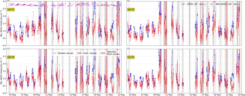
Figure 9 shows an example time series of measured and free cases only. For 30◦ EA, we did not observe any sig-
simulated dSCDs for UBAdi for 30◦ EA. Comparing these nificant change in the agreement of temporal variability (i.e.
values to the VCDs shown in Fig. 6, we observe that the sim- R) between model and MAX-DOAS, whether we compare
ulated dSCDs are higher than the calculated VCDs as shown dSCDs or VCDs. However, significantly more information is
in the previous section, implying dAMFs at 30◦ EA are larger gleaned with respect to the available dSCDs corresponding to
than 1. This is also observed under the cloud-free conditions, all the off-axis EAs at which measurements were performed.
which corroborates the drawback in the geometric approxi- Instead of comparing only one VCD value for a complete el-
mation and assumption of spatial homogeneity in the viewing evation sequence, we include dSCDs corresponding to each
direction. of the elevation angles. For example, in Fig. 11, we observe a
much better agreement between the measured and simulated
Evaluation of simulated dSCDs dSCDs at 3◦ EA, especially on the cloud-free days.
In Fig. 12, we show the comparison of measured and sim-
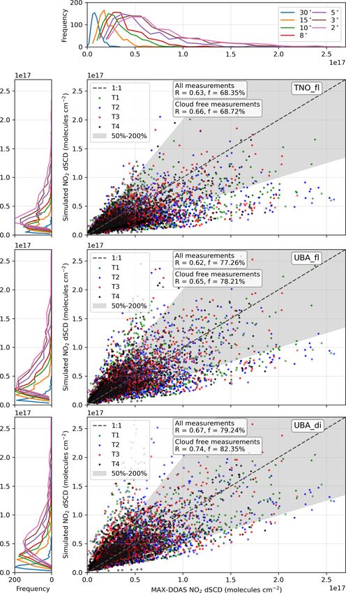
Figure 10 shows the distribution of measured and simulated ulated dSCDs for the three different model set-ups in differ-
dSCDs (different colours for the different model set-ups de- ent panels for all the EAs and all the telescopes. The fre-
scribed in Table 1) for the various elevation angles as box quency distribution of the measured dSCDs at various EAs
and whiskers plots for the four telescopes in separate panels. are shown above the top panel, while those for the simulated
Measurements performed at low EAs have large light paths dSCDs are shown in the panels left of the scatter plot of the
and are more sensitive to air mass close to the surface (higher corresponding model set-ups.
dbAMFs; see Fig. 8); hence, larger dSCDs are observed for We observe a good correlation between the measured and
the low EAs. Surprisingly, we did not observe major differ- simulated dSCDs (R = 0.63, 0.62 and 0.67 for TNOfl , UBAfl
ences in the measured as well as simulated dSCDs among the and UBAdi , respectively), which further improves (R = 0.66,
four telescopes, besides slightly higher values for T2, which 0.65 and 0.74) if the comparison is restricted to cloud-free
points towards the city centre of Mainz and lower values for cases only. Similar to the VMR and VCD comparisons, the
T4, which spans mostly agricultural lands for a distance of best accountability was observed for UBAdi , with ∼ 82 %
10 km. This can partially be explained by the prevailing wind for the simulated dSCDs no less than half and no greater
directions (Fig. 6a), as for most of the time easterly winds than twice the magnitude of the measurements for cloud-free
bring the air mass from the urban locations to the agricul- cases. The frequency distribution of the measured dSCDs
tural lands. follows a right-skewed normal distribution for all the EAs,
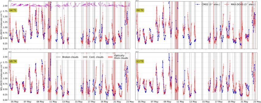
Figures 9 and 11 show example time series of measured which is also represented best by the UBAdi set-up. The
and simulated dSCDs (for UBAdi ) for 30 and 3◦ EAs, re- width of the peak of the frequency distribution broadens
https://doi.org/10.5194/amt-14-5241-2021 Atmos. Meas. Tech., 14, 5241–5269, 2021You can also read