Cloud drop number concentrations over the western North Atlantic Ocean: seasonal cycle, aerosol interrelationships, and other influential factors
←
→
Page content transcription
If your browser does not render page correctly, please read the page content below
Atmos. Chem. Phys., 21, 10499–10526, 2021
https://doi.org/10.5194/acp-21-10499-2021
© Author(s) 2021. This work is distributed under
the Creative Commons Attribution 4.0 License.

Cloud drop number concentrations over the western North Atlantic
Ocean: seasonal cycle, aerosol interrelationships,
and other influential factors
Hossein Dadashazar1 , David Painemal2,3 , Majid Alipanah4 , Michael Brunke5 , Seethala Chellappan6 ,
Andrea F. Corral1 , Ewan Crosbie2,3 , Simon Kirschler7 , Hongyu Liu8 , Richard H. Moore2 , Claire Robinson2,3 ,
Amy Jo Scarino2,3 , Michael Shook2 , Kenneth Sinclair9,10 , K. Lee Thornhill2 , Christiane Voigt7 , Hailong Wang11 ,
Edward Winstead2,3 , Xubin Zeng5 , Luke Ziemba2 , Paquita Zuidema6 , and Armin Sorooshian1,5
1 Department   of Chemical and Environmental Engineering, University of Arizona, Tucson, AZ, USA
2 NASA    Langley Research Center, Hampton, VA, USA
3 Science Systems and Applications, Inc., Hampton, VA, USA
4 Department of Systems and Industrial Engineering, University of Arizona, Tucson, AZ, USA
5 Department of Hydrology and Atmospheric Sciences, University of Arizona, Tucson, AZ, USA
6 Rosenstiel School of Marine and Atmospheric Science, University of Miami, Miami, FL, USA
7 Institute of Atmospheric Physics, German Aerospace Center, Oberpfaffenhofen, Germany
8 National Institute of Aerospace, Hampton, VA, USA
9 NASA Goddard Institute for Space Studies, New York, NY, USA
10 Universities Space Research Association, Columbia, MD, USA
11 Atmospheric Sciences and Global Change Division, Pacific Northwest National Laboratory, Richland, WA, USA

Correspondence: Hossein Dadashazar (hosseind@arizona.edu)

Received: 20 February 2021 – Discussion started: 10 March 2021
Revised: 21 May 2021 – Accepted: 26 May 2021 – Published: 13 July 2021

Abstract. Cloud drop number concentrations (Nd ) over the        days, including reduced sea level pressure and stronger wind
western North Atlantic Ocean (WNAO) are generally high-          speeds. Although aerosols may be more abundant in MAM
est during the winter (DJF) and lowest in summer (JJA), in       and JJA, the conditions needed to activate those particles
contrast to aerosol proxy variables (aerosol optical depth,      into cloud droplets are weaker than in colder months, which
aerosol index, surface aerosol mass concentrations, surface      is demonstrated by calculations of the strongest (weakest)
cloud condensation nuclei (CCN) concentrations) that gen-        aerosol indirect effects in DJF (JJA) based on comparing Nd
erally peak in spring (MAM) and JJA with minima in DJF.          to perturbations in four different aerosol proxy variables (to-
Using aircraft, satellite remote sensing, ground-based in situ   tal and sulfate aerosol optical depth, aerosol index, surface
measurement data, and reanalysis data, we characterize fac-      mass concentration of sulfate). We used three machine learn-
tors explaining the divergent seasonal cycles and furthermore    ing models and up to 14 input variables to infer about most
probe into factors influencing Nd on seasonal timescales. The    influential factors related to Nd for DJF and JJA, with the
results can be summarized well by features most pronounced       best performance obtained with gradient-boosted regression
in DJF, including features associated with cold-air outbreak     tree (GBRT) analysis. The model results indicated that cloud
(CAO) conditions such as enhanced values of CAO index,           fraction was the most important input variable, followed by
planetary boundary layer height (PBLH), low-level liquid         some combination (depending on season) of CAO index and
cloud fraction, and cloud-top height, in addition to winds       surface mass concentrations of sulfate and organic carbon.
aligned with continental outflow. Data sorted into high- and     Future work is recommended to further understand aspects
low-Nd days in each season, especially in DJF, revealed          uncovered here such as impacts of free tropospheric aerosol
that all of these conditions were enhanced on the high-Nd        entrainment on clouds, degree of boundary layer coupling,

Published by Copernicus Publications on behalf of the European Geosciences Union.
10500                   H. Dadashazar et al.: Cloud drop number concentrations over the western North Atlantic Ocean

wet scavenging, and giant CCN effects on aerosol–Nd re-           investigating seasonal cycles of Nd in the North Atlantic re-
lationships, updraft velocity, and vertical structure of cloud    gion found that cloud microphysical properties were primar-
properties such as adiabaticity that impact the satellite esti-   ily dependent on CCN concentrations while cloud macro-
mation of Nd .                                                    physical properties were more dependent on meteorologi-
                                                                  cal conditions (e.g., Sinclair et al., 2020). However, due to
                                                                  the complexity of interactions involved and the co-variability
                                                                  between individual components, the magnitude and sign of
1   Introduction                                                  these feedbacks remain uncertain.
                                                                     This study uses a multitude of datasets to characterize the
Aerosol indirect effects remain the dominant source of un-        Nd seasonal cycle and factors related to Nd variability. The
certainty in estimates of total anthropogenic radiative forc-     structure of the results and discussion is as follows: (i) case
ing (Boucher et al., 2013; Myhre et al., 2013). Central to        study flight highlighting the wide range of Nd in wintertime
these effects is knowledge about cloud drop number con-           and factors potentially affecting that variability; (ii) seasonal
centration (Nd ), as it is the connection between the subset      cycle of Nd and aerosol concentrations based on different
of particles that activate into drops (cloud condensation nu-     proxy variables; (iii) seasonal cycles of factors potentially
clei, CCN) and cloud properties. It is widely accepted that       influential for Nd such as aerosol size distribution, vertical
warm clouds influenced by higher number concentrations of         distribution of aerosol, humidity effects, and aerosol–cloud
aerosol particles have elevated Nd and smaller drops (all else    interactions; (iv) composite analysis of influential factors on
held fixed), resulting in enhanced cloud albedo at fixed liq-     high- and low-Nd days in each season; (v) modeling analysis
uid water path (Twomey, 1977) and potentially suppressed          to probe more deeply into Nd relationships with other param-
precipitation (Albrecht, 1989) and increased vulnerability to     eters for winter and summer seasons; and (vi) discussion of
overlying air resulting from enhanced cloud-top entrainment       other factors relevant to Nd unexplored in this work.
(Ackerman et al., 2004).
   Reducing uncertainty in how aerosols and clouds inter-
act within a given meteorological context requires accurate       2     Methods
estimates of Nd and aerosol concentrations and properties.
Since intensive field studies struggle to obtain broad spatial    2.1     Study region
and temporal coverage of such data, satellite remote sensing
                                                                  We focus on the WNAO, defined here as being bounded by
and reanalysis datasets are relied on for studies examining
                                                                  25–50◦ N and 60–85◦ W. A subset of the results focuses on
intra- and interannual features over large spatial areas. Lim-
                                                                  six individual sub-domains representative of different parts
itations of satellite retrievals are important to recognize. Nd
                                                                  of the WNAO (shown later), with five just off the East Coast
is not directly retrieved but derived using other parameters
                                                                  extending from south to north (south: S; central-south: C-
(e.g., cloud optical depth, cloud drop effective radius, cloud-
                                                                  S; central: C; central-north: C-N; north: N) and one over
top temperature) and with assumptions about cloud adia-
                                                                  Bermuda.
batic growth and Nd being vertically constant (Grosvenor et
al., 2018). Aerosol number concentrations are usually rep-        2.2     Datasets
resented by a columnar parameter such as aerosol optical
depth (AOD) and thus not directly below clouds, which is the      2.2.1    Satellite observations
aerosol layer most likely to interact with the clouds. Further-            (CERES-MODIS/CALIPSO)
more, aerosol data are difficult to retrieve in cloudy columns.
Reanalysis datasets circumvent issues for the aerosol param-      Relevant cloud parameters were obtained from the Clouds
eters as they provide vertically resolved data (e.g., surface     and the Earth’s Radiant Energy System (CERES) edition 4
layer and thus below clouds) and are available for cloudy         products (Minnis et al., 2011, 2020), which are based on
columns.                                                          the application of CERES’s retrieval algorithms on the radi-
   Of special interest in this work is the western North At-      ances measured by the MODerate resolution Imaging Spec-
lantic Ocean (WNAO) where decades of extensive research           troradiometer (MODIS) instrument aboard the Aqua satel-
have been conducted for topics largely unrelated to aerosol–      lite. Aqua observations used to estimate Nd were from the
cloud interactions (Sorooshian et al., 2020), thereby provid-     daytime overpasses of the satellite around 13:30 local time
ing an opportunity for closing knowledge gaps for this area       (LT). Level 3 daily cloud properties at 1◦ × 1◦ spatial res-
in a region with a wide range of aerosol and meteorological       olution (listed in Table 1) were used for the period between
conditions (Corral et al., 2021; Painemal et al., 2021). Past     January 2013 and December 2017 from CERES-MODIS edi-
work showed different seasonal cycles of AOD and Nd in            tion 4 Single Scanning Footprint (SSF) products (Loeb et al.,
this region (Grosvenor et al., 2018; Sorooshian et al., 2019),    2016). The CERES-MODIS SSF Level 3 product includes
which partly motivates this study to unravel why Nd be-           1◦ × 1◦ averaged data according to the cloud-top pressure
haves differently on seasonal timescales. A previous study        of individual pixels: low (heights below 700 hPa), mid-low

Atmos. Chem. Phys., 21, 10499–10526, 2021                                            https://doi.org/10.5194/acp-21-10499-2021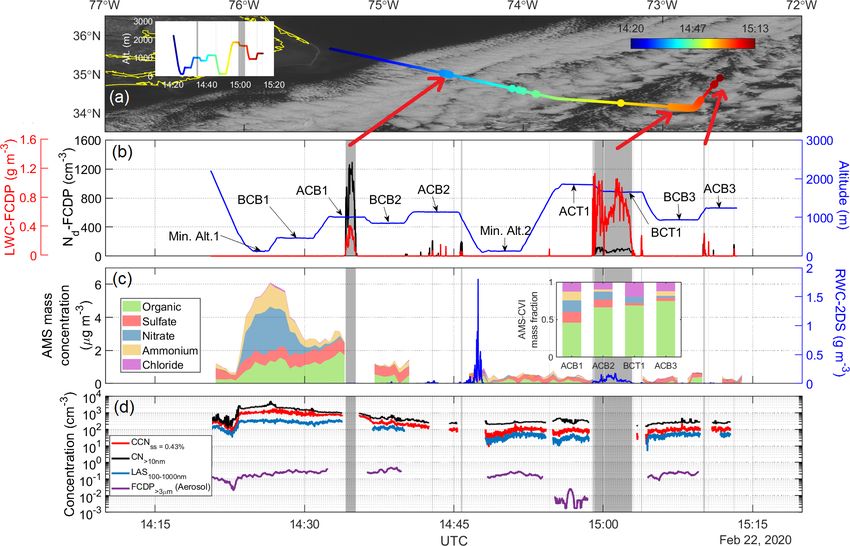
H. Dadashazar et al.: Cloud drop number concentrations over the western North Atlantic Ocean                               10501

(heights within 700–500 hPa), mid-high (heights within 500–        tem (Buchard et al., 2017; Randles et al., 2017). Aerosols in
300 hPa), and high (heights above 300 hPa) level clouds. For       MERRA-2 are simulated with a radiatively coupled version
this study, we only use low-cloud averages.                        of the Goddard Chemistry, Aerosol, Radiation, and Transport
   Nd is estimated based on an adiabatic cloud model               model (GOCART; Chin et al., 2002; Colarco et al., 2010).
(Grosvenor et al., 2018):                                          GOCART treats the sources, sinks, and chemistry of 15 ex-
        √                                                         ternally mixed aerosol mass mixing ratio tracers, which in-
         5 fad Cw τ 1/2

Nd =                       ,                             (1)       clude sulfate, hydrophobic and hydrophilic black and organic
       2π k Qext ρw re5                                            carbon, dust (five size bins), and sea salt (five size bins).
where τ is cloud optical depth and re is cloud drop effective      MERRA-2 includes assimilation of bias-corrected Collec-
radius, both of which are obtained from CERES-MODIS for            tion 5 MODIS AOD, bias-corrected AOD from the Ad-
low-level (i.e., surface to 700 hPa) liquid clouds. Qext is the    vanced Very High Resolution Radiometer (AVHRR) instru-
unitless extinction efficiency factor, assumed to be 2 for liq-    ments, AOD retrievals from the Multiangle Imaging Spectro-
uid cloud droplets, and ρw is the density of water (1 g cm−3 ).    Radiometer (MISR) over bright surfaces, and ground-based
Methods described in Painemal (2018) were used to estimate         Aerosol Robotic Network (AERONET) direct measurements
parameters in Eq. (1) as follows. (i) Adiabatic water lapse        of AOD (Gelaro et al., 2017). In this study we used total
rate (Cw ) was determined using cloud-top pressure and tem-        and speciated (i.e., sea salt, dust, black carbon, organic car-
perature provided by CERES-MODIS. (ii) The Nd estima-              bon, and sulfate) AOD at 550 nm between January 2013 and
tion is often corrected for the sub-adiabatic profile by ap-       December 2017 at times relevant to Aqua’s overpass time
plying the adiabatic value (fad ), but in this work, a value       (13:30 LT). Aerosol index was calculated as the product of
of fad = 1 was assumed due to both lack of consensus on            AOD and the Ångström parameter. MERRA-2 also provides
its value and its relatively minor impact on Nd estimation         surface mass concentrations of aerosol species including sea
(Grosvenor et al., 2018). (iii) k is the parameter represent-      salt, dust, black carbon, organic carbon, and sulfate, which
ing the width of the droplet spectrum and was assumed to           were used as a measure of aerosol levels in the planetary
be 0.8 over the ocean. Statistics of Nd are often estimated        boundary layer (PBL).
after screening daily observations based on cloud fractions           MERRA-2 data were also used for environmental vari-
(Wood, 2012; Grosvenor et al., 2018). The purpose of such          ables including both thermodynamic (e.g., temperature and
filters is to reduce the uncertainties associated with the es-     relative humidity) and dynamic parameters (e.g., sea level
timation of Nd (Eq. 1) driven by the errors in the retrieval       pressure (SLP) and geopotential heights) (Gelaro et al., 2017)
of re and τ from MODIS’s observed reflectance in a highly          listed in Table 1. Bilinear interpolation was applied to trans-
heterogeneous cloud field. However, this may inadvertently         fer all MERRA-2 variables (Table 1) from their original
mask the effects of cloud regime on aerosol–cloud interac-         0.5◦ × 0.625◦ spatial resolution to the equivalent 1◦ × 1◦ grid
tions by only including certain low-level cloud types in the       in CERES-MODIS Level 3 data.
analyses (e.g., closed-cell stratocumulus). Therefore, we use
all Nd data regardless of cloud fraction with exceptions be-       2.2.3   Precipitation data
ing Sects. 3.5 and 4.2 where a filter of low-level liquid cloud
fraction (i.e., CFlow-liq. ≥ 0.1) was applied.                     Daily precipitation data were obtained from the Precipitation
    The Cloud-Aerosol Lidar with Orthogonal Polarization           Estimation from Remotely Sensed Information using Arti-
(CALIOP) instrument aboard the Cloud-Aerosol Lidar and             ficial Neural Networks–Climate Data Record (PERSIANN-
Infrared Pathfinder Satellite Observations (CALIPSO) pro-          CDR) data product (Ashouri et al., 2015; Nguyen et al.,
vides data on the vertical distribution of aerosols (Winker et     2018). Bilinear interpolation was applied to convert the
al., 2009). Nighttime extinction profiles were acquired from       PERSIANN-CDR data from their native spatial resolution
Level 2 version 4.20 products (i.e., 5 km aerosol profile data),   (i.e., 0.25◦ × 0.25◦ ) to equivalent 1◦ × 1◦ grids in CERES-
between January 2013 and December 2017. We averaged the            MODIS Level 3 data. It is important to note that we use
Level 2 daily extinctions in different 4◦ × 5◦ sub-domains         daily averaged PERSIANN-CDR precipitation and, there-
(shown later) to obtain the seasonal profiles after applying       fore, there is some temporal mismatch with the daily Nd
the screening scheme outlined in Tackett et al. (2018).            value from MODIS-Aqua that comes at one time of the day.
                                                                   This can contribute to some level of uncertainty for the dis-
2.2.2   MERRA-2                                                    cussions based on analyses involving relationships between
                                                                   precipitation and Nd .
Aerosol data were obtained from the Modern-Era Retro-
spective Analysis for Research and Applications-Version 2          2.2.4   Surface-based CCN data
(MERRA-2) (Gelaro et al., 2017). MERRA-2 is a multi-
decadal reanalysis where meteorological and aerosol obser-         Cloud condensation nuclei (CCN) data were obtained from
vations are jointly assimilated into the Goddard Earth Ob-         the U.S. Department of Energy’s Two-Column Aerosol
servation System version 5 (GEOS-5) data assimilation sys-         Project (TCAP) (Berg et al., 2016) to examine the seasonal

https://doi.org/10.5194/acp-21-10499-2021                                        Atmos. Chem. Phys., 21, 10499–10526, 2021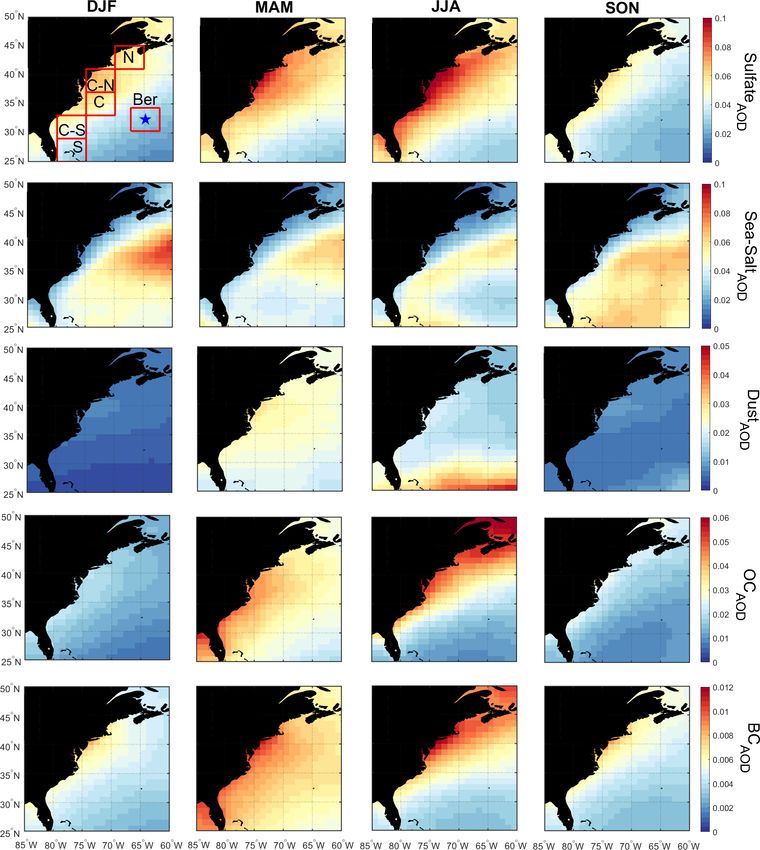
H. Dadashazar et al.: Cloud drop number concentrations over the western North Atlantic Ocean
https://doi.org/10.5194/acp-21-10499-2021
Table 1. Summary of various data products used in this study.
Parameter Data source Spatial Vertical level Date range Spatial area Temporal
resolution resolution
Cloud optical thickness CERES-MODIS 1◦ × 1◦ NA 1 January 2013–31 December 2017 25–50◦ N, 60–85◦ W Daily
Cloud effective radius CERES-MODIS 1◦ × 1◦ NA 1 January 2013–31 December 2017 25–50◦ N, 60–85◦ W Daily
Cloud fraction CERES-MODIS 1◦ × 1◦ NA 1 January 2013–31 December 2017 25–50◦ N, 60–85◦ W Daily
Cloud-top temperature CERES-MODIS 1◦ × 1◦ NA 1 January 2013–31 December 2017 25–50◦ N, 60–85◦ W Daily
Cloud effective height CERES-MODIS 1◦ × 1◦ NA 1 January 2013–31 December 2017 25–50◦ N, 60–85◦ W Daily
Cloud-top pressure CERES-MODIS 1◦ × 1◦ NA 1 January 2013–31 December 2017 25–50◦ N, 60–85◦ W Daily
Precipitation PERSIANN-CDR 1◦ × 1◦ NA 1 January 2013–31 December 2017 25–50◦ N, 60–85◦ W Daily
Aerosol extinction (532 nm) CALIPSO/CALIOP 5 km NA 1 January 2013–31 December 2017 25–50◦ N, 60–85◦ W Daily
Total aerosol extinction AOT (550 nm) MERRA-2 1◦ × 1◦ NA 1 January 2013–31 December 2017 25–50◦ N, 60–85◦ W Daily
Total aerosol Ångström parameter (470–870 nm) MERRA-2 1◦ × 1◦ NA 1 January 2013–31 December 2017 25–50◦ N, 60–85◦ W Daily
Sulfate extinction AOT (550 nm) MERRA-2 1◦ × 1◦ NA 1 January 2013–31 December 2017 25–50◦ N, 60–85◦ W Daily
Sea salt extinction AOT (550 nm) MERRA-2 1◦ × 1◦ NA 1 January 2013–31 December 2017 25–50◦ N, 60–85◦ W Daily
Dust extinction AOT (550 nm) MERRA-2 1◦ × 1◦ NA 1 January 2013–31 December 2017 25–50◦ N, 60–85◦ W Daily
Organic carbon extinction AOT (550 nm) MERRA-2 1◦ × 1◦ NA 1 January 2013–31 December 2017 25–50◦ N, 60–85◦ W Daily
Black carbon extinction AOT (550 nm) MERRA-2 1◦ × 1◦ NA 1 January 2013–31 December 2017 25–50◦ N, 60–85◦ W Daily
Sulfate surface mass concentration MERRA-2 1◦ × 1◦ Surface 1 January 2013–31 December 2017 25–50◦ N, 60–85◦ W Daily
Sea salt surface mass concentration MERRA-2 1◦ × 1◦ Surface 1 January 2013–31 December 2017 25–50◦ N, 60–85◦ W Daily
Dust surface mass concentration MERRA-2 1◦ × 1◦ Surface 1 January 2013–31 December 2017 25–50◦ N, 60–85◦ W Daily
Organic carbon surface mass concentration MERRA-2 1◦ × 1◦ Surface 1 January 2013–31 December 2017 25–50◦ N, 60–85◦ W Daily
Black carbon surface mass concentration MERRA-2 1◦ × 1◦ Surface 1 January 2013–31 December 2017 25–50◦ N, 60–85◦ W Daily
1◦ × 1◦ 25–50◦ N, 60–85◦ W
Atmos. Chem. Phys., 21, 10499–10526, 2021
Sea level pressure MERRA-2 Surface 1 January 2013–31 December 2017 Daily
Geopotential height MERRA-2 1◦ × 1◦ 850 hPa 1 January 2013–31 December 2017 25–50◦ N, 60–85◦ W Daily
Sea surface temperature MERRA-2 1◦ × 1◦ Sea surface 1 January 2013–31 December 2017 25–50◦ N, 60–85◦ W Daily
Air temperature MERRA-2 1◦ × 1◦ Surface, 850, 700 hPa 1 January 2013–31 December 2017 25–50◦ N, 60–85◦ W Daily
Relative humidity MERRA-2 1◦ × 1◦ 1000–500 hPa 1 January 2013–31 December 2017 25–50◦ N, 60–85◦ W Daily
Wind speed MERRA-2 1◦ × 1◦ 2 m, 950 hPa 1 January 2013–31 December 2017 25–50◦ N, 60–85◦ W Daily
Planetary boundary layer height MERRA-2 1◦ × 1◦ NA 1 January 2013–31 December 2017 25–50◦ N, 60–85◦ W Daily
Vertical pressure velocity MERRA-2 1◦ × 1◦ 800 hPa 1 January 2013–31 December 2017 25–50◦ N, 60–85◦ W Daily
Aerosol/cloud Airborne: ACTIVATE – NA 22 February 2020 34.08–37.16◦ N, 72.31–76.64◦ W 1s
CCN-Cape Cod Ground-based measurement Point measurement Surface 16 July 2012–4 May 2013 41.67◦ N, 70.30◦ W 1s
10502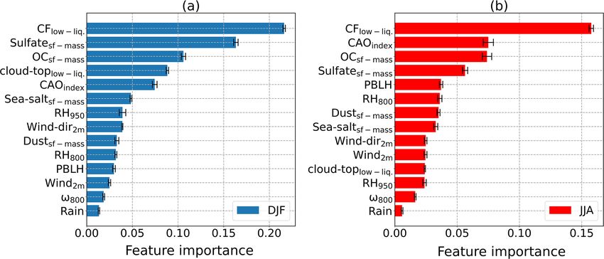
H. Dadashazar et al.: Cloud drop number concentrations over the western North Atlantic Ocean                                 10503

variations in CCN number concentration at a representative         measurement system (TAMMS) for winds and temperature
site by Cape Cod, Massachusetts (41.67◦ N, 70.30◦ W), over         (Thornhill et al., 2003).
the US East Coast. TCAP was a campaign conducted be-                  CCN, LAS, CPC, and AMS data were collected down-
tween June 2012 and June 2013 to investigate aerosol opti-         stream of an isokinetic double diffuser inlet (BMI, Inc.),
cal and physicochemical properties and interactions between        whereas the AMS and LAS also sampled downstream of a
aerosols and clouds (Berg et al., 2016; Liu and Li, 2019).         counterflow virtual impactor (CVI) inlet (BMI, Inc.) when in
CCN data were available between July 2012 and May 2013 at          cloud (Shingler et al., 2012). However, a filter was applied
multiple supersaturations with some gaps in the data collec-       to remove LAS data when the CVI inlet was used. Measure-
tion (i.e., November–December); for simplicity, we focused         ments from the CCN counter, LAS, CPC, and FCDP-aerosol
on CCN data measured at a single supersaturation of 1 %            are only shown in cloud-free and rain-free conditions, dis-
owing to relatively better data coverage compared to lower         tinguished by LWC < 0.05 g m−3 and RWC < 0.05 g m−3 ,
supersaturations. We note that this higher supersaturation is      respectively, and also excluding data collected 20 s before
not necessarily representative of that relevant to the clouds of   and after evidence of rain or cloud. Estimation of supermi-
interest but is still insightful for understanding the seasonal    crometer particles from FCDP measurements was performed
cycle of CCN concentration. The qualitative seasonal cycle         after conducting the following additional screening steps to
of CCN concentration at 1 % matches those at lower super-          minimize cloud droplet artifacts: (i) only samples with RH
saturations (e.g., 0.15 %–0.8 %).                                  < 98 % were included; (ii) data collected during ACB and
                                                                   BCT legs were excluded. CCN, LAS, CPC, and AMS mea-
                                                                   surements are reported at standard temperature and pressure
2.2.5   Airborne in situ data
                                                                   (i.e., 273 K and 101.325 kPa) while FCDP and 2DS measure-
                                                                   ments correspond to ambient conditions.
We used airborne in situ data collected during the fifth re-
search flight (RF05) of the Aerosol Cloud meTeorology In-          2.3   Regression analyses
teractions oVer the western ATlantic Experiment (ACTI-
VATE) campaign. One flight is used both for simplicity and         Regression modeling was conducted to investigate relation-
because it embodied conditions relevant to the discussion of       ships between environmental variables and Nd . The gradient-
other results. The mission concept involves joint flights be-      boosted regression trees (GBRT) model, classified as a ma-
tween the NASA Langley UC-12 King Air and HU-25 Fal-               chine learning (ML) model, is used, consisting of several
con such that the former flies around 8–10 km, and the lat-        weak learners (i.e., regression trees with a fixed size) that are
ter flies in the boundary layer to simultaneously collect data     designed and subsequently trained to improve prediction ac-
on aerosol, cloud, gas, and meteorological parameters in the       curacy by fitting the model’s trees on residuals rather than re-
same column (Sorooshian et al., 2019). The Falcon flew in          sponse values (Hastie et al., 2009). Desirable characteristics
a systematic way to collect data at different vertical regions     of the GBRT model include both its capacity to capture non-
relative to cloud, including the following of relevance to this    linear relationships and being less vulnerable to overfitting
study: BCB – below cloud base; ACB – above cloud base;             (Persson et al., 2017; Fuchs et al., 2018; Dadashazar et al.,
BCT – below cloud top; and Min. Alt – minimum altitude             2020). Two separate GBRT models were trained using daily
the plane flies at (∼ 150 m).                                      CERES-MODIS Nd data (1◦ × 1◦ ) in winter (DJF) and sum-
   This study makes use of the HU-25 Falcon data from              mer (JJA) to reveal potential variables impacting Nd . Winter
the following instruments: fast cloud droplet probe (FCDP;         and summer are chosen as they exhibit the highest and lowest
Dp ∼ 3–50 µm) (SPEC Inc.) aerosol and cloud droplet size           Nd concentrations, respectively, among all seasons over the
distributions for quantification of cloud liquid water con-        WNAO.
tent (LWC), Nd , and aerosol number concentrations with               Many variables were picked as input parameters (Ta-
Dp exceeding 3 µm in cloud-free air (termed FCDP-aerosol);         ble 2) for the GBRT model, categorized as being aerosol, dy-
two-dimensional stereo (2DS; Dp ∼ 28.5–1464.9 µm) (SPEC            namic/thermodynamic, or cloud variables. Aerosol parame-
Inc.) probe for estimation of rain water content (RWC)             ters included MERRA-2 surface mass concentrations for sul-
by integrating raindrop (Dp ≥ 39.9 µm) size distributions;         fate, sea salt, dust, and organic carbon. Black carbon con-
cloud condensation nuclei (CCN; DMT) counter for CCN               centration was removed from input parameters because of
number concentrations; laser aerosol spectrometer (LAS;            its high correlation (R 2 = 0.6) with organic carbon. The fol-
TSI model 3340) and condensation particle counter (CPC;            lowing is the list of thermodynamic/dynamic input param-
TSI model 3772) for aerosol number concentrations with             eters derived from MERRA-2: vertical pressure velocity at
Dp between 0.1–1 µm and above 10 nm, respectively; high-           800 hPa (ω800 ), planetary boundary layer height (PBLH),
resolution time-of-flight aerosol mass spectrometer (AMS;          cold-air outbreak (CAO) index, wind speed and wind direc-
Aerodyne) for submicrometer non-refractory aerosol compo-          tion at 2 m (wind2 m and wind-dir2 m ), and relative humidity
sition (DeCarlo et al., 2008), operated in 1 Hz Fast-MS mode       (RH) in the PBL and free troposphere represented by RH950
and averaged to 25 s time resolution; and turbulent air-motion     and RH800 , respectively. CAO index is defined as the dif-

https://doi.org/10.5194/acp-21-10499-2021                                        Atmos. Chem. Phys., 21, 10499–10526, 2021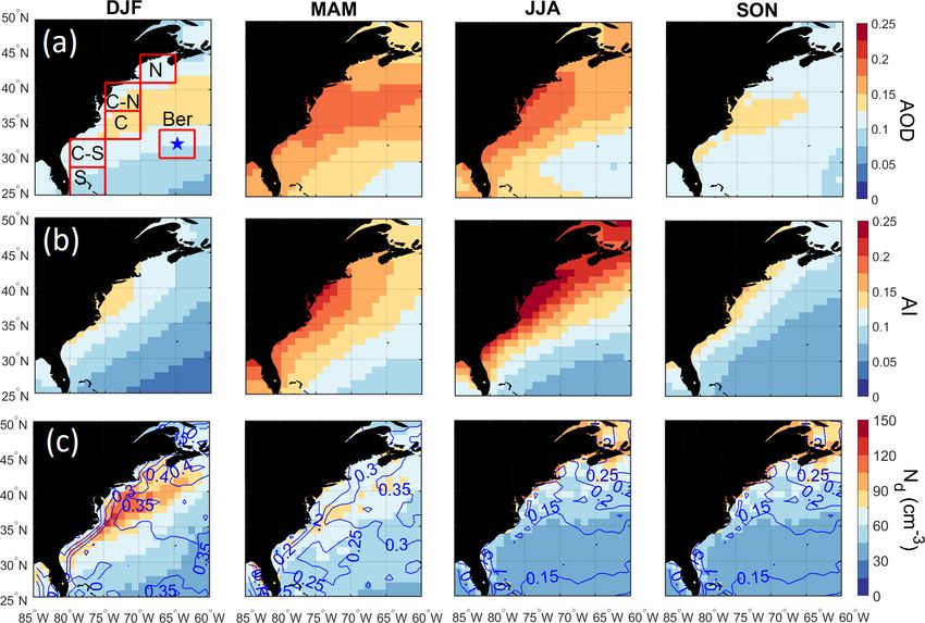
10504                   H. Dadashazar et al.: Cloud drop number concentrations over the western North Atlantic Ocean

Table 2. List of input parameters used as predictor variables in the GBRT and linear models. Variables are grouped into three general
categories.

                                                    Parameter
                            Aerosol                 Sulfate surface mass concentration (Sulfatesf-mass )
                                                    Sea salt surface mass concentration (Sea-saltsf-mass )
                                                    Dust surface mass concentration (Dustsf-mass )
                                                    Organic carbon surface mass concentration (OCsf-mass )
                            Cloud                   Low-level liquid cloud fraction (CFlow-liq. )
                                                    Low-level liquid cloud-top effective height (Cloud-toplow-liq. )
                                                    Precipitation rate (Rain)
                            Dynamic/                                                        ∗ -θ
                                                    Cold-air outbreak index (CAOindex ): θskt   850
                            thermodynamic           Relative humidity at 950 hPa (RH950 )
                                                    Relative humidity at 800 hPa (RH800 )
                                                    Vertical pressure velocity at 800 hPa (ω800 )
                                                    Wind speed at 2 m (Wind2 m )
                                                    Wind direction at 2 m (Wind-dir2 m )
                                                    Planetary boundary layer height (PBLH)
                          ∗ Skin potential temperature.

ference between skin potential temperature (θskt ) and air po-               tation of the results was done with the aid of accumulated
tential temperature at 850 hPa (θ850 ) (Papritz et al., 2015).               local effect (ALE) plots, which are specifically designed to
Updraft velocity plays a crucial role in the activation of                   be unbiased to the correlated input variables (Apley and Zhu,
aerosol into cloud droplets in warm clouds (Feingold, 2003;                  2020). ALE plots illustrate the influence of input variables
Reutter et al., 2009). Since the direct representation of up-                on the response parameter in ML models. The ALE value for
draft speed is not available from reanalysis data, near-surface              a particular variable s at a specific value of xs (i.e., fs,ALE
wind speed (i.e., wind2 m ) is used as a representative proxy                (xs )) can be calculated as follows:
parameter as an input parameter to the regression models.
CERES-MODIS cloud parameters include liquid cloud frac-                                       Zxs Z
tion and cloud-top height for low-level clouds. In addition,                 fs,ALE (xs ) =           f s (zs , xc ) P (xc |zs ) dxc dzs − constant, (2)
PERSIANN-CDR daily precipitation (Rain) was included as                                    z0,1 xc
a relevant cloud parameter.
   Data were split into two sets: training/validation (70 %)                 where f s (zs xc ) is the gradient of model’s response with re-
and testing (30 %). Five-fold cross-validation was imple-                    spect to variable s (i.e., local effect) and P (xc |zs ) is the
mented to train the GBRT model using the training/validation                 conditional distribution of xc , where c denotes the other in-
data. Furthermore, both performance and generalizability of                  put variables rather than s, and xc is the associated point
the trained models were tested via the aid of the test set,                  in the variable space of c. z0,1 is chosen arbitrarily below
which was not used in the training process. Hyperparame-                     the smallest observation of feature s (Apley and Zhu, 2020).
ters of the GBRT models were optimized through a combi-                      The steps in Eq. (2) can be summarized as follows (Molnar,
nation of both random and grid search methods. Table S1 in                   2019; Apley and Zhu, 2020): (i) the average change in the
the Supplement shows the list of important hyperparameters                   model’s prediction is calculated using the conditional distri-
of the GBRT model and associated ranges tested via random                    bution of features; (ii) the average change will then be ac-
and grid search methods. The optimized model hyperparam-                     cumulated by integrating it over feature s; and (iii) a con-
eters can also be found in Table S1. The GBRT models were                    stant will be subtracted to vertically center (i.e., the aver-
performed using the scikit-learn module designed in Python                   age of ALE becomes zero) the ALE plot. The aforemen-
(Pedregosa et al., 2011).                                                    tioned steps, although seemingly complex, assure the avoid-
   The regression analyses were not performed solely to con-                 ance of undesired extrapolation (especially an issue for cor-
struct and provide a highly accurate model useful for pre-                   related variables) occurring in alternative approaches such as
diction, but rather to disclose and examine the possible ef-                 partial dependence (PD) plots. The value of fs,ALE (xs ) can
fects of the relevant input variables on Nd considering all the              be viewed as the difference between the model’s response
shortcomings of such analyses. For instance, there is some                   at xs and the average prediction. We used the source code
level of interdependency between input variables. To reduce                  available in https://github.com/blent-ai/ALEPython (Jumelle
unwanted consequences of correlated features, the interpre-                  et al., 2021) for the calculation of ALE plots.

Atmos. Chem. Phys., 21, 10499–10526, 2021                                                       https://doi.org/10.5194/acp-21-10499-2021
H. Dadashazar et al.: Cloud drop number concentrations over the western North Atlantic Ocean 10505
3 Results and discussion number concentration and AMS non-refractory aerosol for
the two BCB legs were as follows: 277 cm−3 /3.64 µg m−3
3.1 Aircraft case study of Nd gradient (BCB1) and 48 cm−3 /0.42 µg m−3 (BCB3). The higher Nd
value (1298 cm−3 ) relative to LAS aerosol concentration
ACTIVATE Research Flight 5 (RF05) on 22 February 2020 (424 cm−3 ) at the near-shore point is suggestive of aerosol
demonstrates the wide range in Nd offshore in the PBL smaller than 0.1 µm activating into drops. This is sup-
(1.6 km) over the WNAO (Fig. 1). On this day, the ACTI- ported by the fact that both CCN (supersaturation = 0.43 %)
VATE study region was dominated by a surface high-pressure and CPC number concentrations with Dp > 10 nm exhibited
system centered over the southeastern US, with a signifi- mean values of 980 and 1723 cm−3 in the BCB1 leg, respec-
cant ridge axis extending from the main high to the east- tively, dropping to 98 and 260 cm−3 in the BCB3 leg. For the
northeast off the Virginia–North Carolina coast and into the duration of the flight portion shown in Fig. 1, supermicrome-
WNAO. Aloft, the flight region was located in northwest- ter concentrations varied over 2 orders of magnitude (0.002–
erly flow behind a trough offshore. This setup led to subsi- 0.51 cm−3 ) and expectedly did not exhibit a pronounced off-
dence in the region and generally clear skies, except where shore gradient as it is naturally emitted from the ocean.
scattered to broken marine boundary layer clouds formed Closer to shore during the Min. Alt. 1 leg, nitrate was
along and east of the Gulf Stream. The 2 d NOAA HYSPLIT the dominant aerosol species (∼ 70 % mass fraction). Far-
(Stein et al., 2015; Rolph et al., 2017) back trajectories us- ther offshore during both the BCB1 leg and cloud-free por-
ing the “model vertical velocity” method and “REANALY- tion of the ACB1 leg, organics were the dominant constituent
SIS” meteorology data indicate air in the flight region (be- (∼ 46 % mass fraction), whereas farther during the BCB3
tween 0–3 km) had wrapped around the surface high from leg, the mean mass fraction of sulfate was the highest (75 %).
the north and left the New England coast 12–24 h before- Droplet residual particle data show a greater contribution of
hand (with a descending profile). Along the flight segment organics farther offshore, increasing from 46 % to 75 % be-
shown, winds were approximately 6 m s−1 , out of the north- tween the ACB1 and ACB3 legs, respectively. These compo-
northwest during the initial descent, Min. Alt. 1, and BCB1 sition results, albeit limited to the non-refractory portion of
legs and primarily from the northeast for the other sections submicrometer aerosol particles, reveal significant changes
of the flight. Sea surface temperatures were 6–9 ◦ C near the with distance offshore indicative of varying chemical prop-
coast during the descent and Min. Alt. 1 leg (readers are re- erties of particles activating into droplets.
ferred to Fig. 1’s caption for the definition of different legs); The cloudy portions of ACB1 are characterized as having
21–25 ◦ C over the Gulf Stream during the BCB1, ACB1, and little or no rain with a maximum RWC value of 0.02 g m−3
BCB2 legs; and 17–20 ◦ C for the remainder of the flight seg- and mean value of 0.003 g m−3 . There is a notable RWC peak
ment shown. The majority of the segment was in or below the at the beginning of the Min. Alt. 2 leg, reaching as high as
boundary layer clouds, with cloud base around 900–1100 m 1.81 g m−3 associated with clouds aloft. The precipitation oc-
and cloud top around 1750 m. Note that the initial BCB1 leg currence was also evident in a subsequent BCT1 leg where
was much lower at around 460 m, likely reflecting a shal- RWC reached as high as 0.18 g m−3 . GOES satellite imagery
lower marine boundary layer and cloud base near the much of the study region (Fig. 1) also reflects the effect of precipi-
colder waters close to the coast. Static air temperature ranged tation on cloud morphology where clouds farther offshore re-
between 0–10 ◦ C, except for the BCT1 leg where tempera- semble open-cell structures. Associated scavenging of parti-
tures were around −2.3 ◦ C. cles through the washout process is presumed to contribute to
Nd values from the FCDP ranged from a maximum value the decline in aerosol concentrations with distance offshore.
of 1298 cm−3 closer to the coast during the ACB1 leg Figure 1 shows changes in aerosol characteristics coinci-
(35.00◦ N, 74.55◦ W) to a minimum of 19 cm−3 farther away dent with the large gradient in Nd . While ACTIVATE air-
in the BCT1 leg (34.32◦ N, 72.73◦ W). The minimum Nd borne data collection is ongoing to build flight statistics over
value in the ACB3 leg was 85 cm−3 (34.11◦ N, 72.80◦ W), multiple years, the wide changes in microphysical properties
which is a fairer comparison to the ACB1 leg compared to in RF05 motivate looking at other datasets with broader spa-
the BCT1 leg in terms of being closer to cloud base. The tiotemporal coverage to learn about potential seasonally de-
mean Nd values (cm−3 ) in the cloudy portions of the ACB1, pendent drivers of Nd , including meteorological parameters
BCT1, and ACB3 legs were as follows: 849, 77, and 143. that vary throughout the year. Furthermore, other datasets can
Based on the nearest BCB legs adjacent to the maxi- provide insight into the source(s) of seasonal discrepancy be-
mum and minimum Nd values (BCB1 = 35.31◦ N, 74.95◦ W; tween columnar aerosol remote sensing parameters and Nd .
BCB3 = 34.41◦ N, 72.70◦ W), there was a significant off-
shore gradient in LAS submicrometer particle number con- 3.2 Seasonal cycles of Nd and AOD
centration and AMS non-refractory aerosol mass, rang-
ing from as high as 424 cm−3 and 5.60 µg m−3 (dur- Figure 2 illustrates the seasonal differences in MERRA-
ing BCB1) to as low as 21 cm−3 and 0.27 µg m−3 (dur- 2 AOD and CERES-MODIS Nd over the WNAO that
ing BCB3). The mean values of submicrometer particle partly motivate this study. Seasonal mean values (±
https://doi.org/10.5194/acp-21-10499-2021 Atmos. Chem. Phys., 21, 10499–10526, 202110506 H. Dadashazar et al.: Cloud drop number concentrations over the western North Atlantic Ocean Figure 1. Time series of selected parameters measured by the HU-25 Falcon aircraft during a selected segment of RF05 on 22 February 2020. (a) Overlayed flight track on GOES 16 visible imagery obtained at 14:55:04 UTC. (b) Altitude, cloud liquid water content (LWC), and Nd , with the latter two obtained from the FCDP. (c) Rain water content (RWC) measured by 2DS probe, AMS speciated mass concentration in cloud/rain-free air, and AMS mass fractions for droplet residual particles in cloud as measured downstream of a CVI inlet. (d) Number concentrations for CCN at 0.43 % supersaturation and particles for three diameter ranges: above 10 nm (CPC), 100–1000 nm (LAS), and above 3 µm (FCDP). Shaded gray areas in panels (b)–(d) highlight cloudy periods identified as having LWC ≥ 0.05 g m−3 . Locations of the cloudy regions are pointed to with red arrows in the satellite imagery. Level legs are defined as follows: BCB: below cloud base; ACB: above cloud base; Min. Alt.: minimum altitude the plane flies at (∼ 150 m); ACT: above cloud top; BCT: below cloud top. standard deviation) of AOD/Nd (cm−3 ) were as follows pattern owing to continental sources. Dust and sea salt have for the entire WNAO: DJF = 0.11 ± 0.03/64.1 ± 18.0; different spatial distributions with the former derived from MAM = 0.16 ± 0.03/60.4 ± 13.1; sources such as North Africa leading to enhanced AODs JJA = 0.15 ± 0.03/49.1 ± 10.1; and < 30◦ N in particular in JJA and sea salt being enhanced SON = 0.11 ± 0.03/50.3 ± 13.9. In contrast to AOD, offshore in particular in JJA. Nd values and low-cloud fraction (Fig. 2c) were highest in Table 3 probes deeper into individual WNAO sub-domains DJF and lowest in JJA. DJF showed notably high Nd near to compare seasonal AOD and Nd values. For the six sub- the coast, qualitatively consistent with the airborne data. The domains in Fig. 2, MERRA-2 AOD peaks in MAM and seasons with the greatest AOD values, accompanied by the JJA, while Nd peaks in DJF. The Bermuda sub-domain most pronounced spatial gradient offshore, were JJA and was unique in that mean Nd was slightly higher in MAM MAM. The offshore gradient owes to continental pollution (53 cm−3 ) compared to DJF (48 cm−3 ). We attribute the outflow (Corral et al., 2021, and references therein). In slightly different seasonal cycle over Bermuda to its remote contrast, DJF and SON exhibited lower AOD values with a nature, leading to differences in meteorology and aerosol distinct area of higher AOD values offshore between ∼ 35– sources between seasons. 40◦ N accounted for by sea salt. MERRA-2 speciated AOD One factor that could bias AOD towards higher values data (Fig. 3) indicate that sea salt and sulfate dominate total with disproportionately less impact on Nd is aerosol hy- AOD regardless of season and that sulfate, organic carbon, groscopic growth in humid conditions. Table 3 summarizes and black carbon most closely follow the offshore gradient mean MERRA-2 RH values in the PBL and free troposphere Atmos. Chem. Phys., 21, 10499–10526, 2021 https://doi.org/10.5194/acp-21-10499-2021
H. Dadashazar et al.: Cloud drop number concentrations over the western North Atlantic Ocean                                    10507

Figure 2. Seasonal spatial maps for (a) MERRA-2 aerosol optical depth (AOD), (b) MERRA-2 aerosol index (AI), and (c) cloud drop
number concentration (Nd ) over the western North Atlantic Ocean (WNAO). Contours in panel (c) represent low-level (cloud-top pressure
> 700 hPa) liquid cloud fraction (CFlow-liq. ). Cloud data are based on daily Level 3 data from CERES-MODIS. The maps are based on data
between January 2013 and December 2017. The boxes in the top left panel represent sub-domains examined in more detail throughout the
study, with the blue star denoting Bermuda.

Table 3. Average drop number concentration (Nd ), MERRA-2 AOD, and vertically resolved AOD characteristics from CALIOP for each
season over the sub-domains shown in Fig. 2. Total CALIOP AOD is shown outside parentheses, and numbers inside are the percent AOD
fraction in the planetary boundary layer followed by in the free troposphere. Also shown are PBLHs (shown in Fig. 4) and the relative
humidity in the PBL and FT.

                                       S           C-S              C            C-N              N       Bermuda
                   AODMERRA-2 /Nd (cm−3 )
                   DJF           0.10/56        0.11/74        0.13/91        0.12/97        0.11/78        0.10/48
                   MAM           0.14/55        0.17/62        0.18/72        0.19/75        0.16/70        0.14/53
                   JJA           0.14/41        0.16/43        0.17/47        0.19/68        0.17/73        0.11/37
                   SON           0.11/42        0.12/53        0.13/62        0.13/74        0.11/73        0.11/36
                   AODCALIOP (%PBL, %FT)
                   DJF      0.11 (64,36)   0.11 (67,33)   0.15 (68,32)   0.09 (61,39)   0.13 (59,41)   0.14 (72,28)
                   MAM      0.11 (54,46)   0.10 (53,47)   0.12 (58,42)   0.10 (30,70)   0.07 (30,70)   0.12 (58,42)
                   JJA      0.11 (53,47)   0.11 (44,56)   0.10 (46,54)   0.11 (20,80)   0.08 (11,89)   0.08 (49,51)
                   SON      0.09 (63,37)   0.10 (57,43)   0.10 (65,35)   0.08 (47,53)   0.07 (35,65)   0.10 (69,31)
                   PBLH (m)/RHPBL (%)/RHFT (%)
                   DJF       1018/78/37     1156/76/43     1364/79/46     1013/76/52      926/76/58     1198/80/43
                   MAM        903/77/41      955/72/43     1043/75/48      722/72/53      568/79/55      966/79/50
                   JJA        775/81/62      725/81/60      697/81/59      481/78/53      351/85/55      713/82/58
                   SON       1018/80/50     1094/76/45     1181/76/42      825/71/43      593/77/51     1095/81/48

https://doi.org/10.5194/acp-21-10499-2021                                            Atmos. Chem. Phys., 21, 10499–10526, 2021
10508 H. Dadashazar et al.: Cloud drop number concentrations over the western North Atlantic Ocean
Figure 3. Seasonal maps of MERRA-2 speciated AOD based on data between January 2013 and December 2017. The boxes in the top left
panel represent sub-domains examined in more detail throughout the study, with the blue star denoting Bermuda.
(FT). Results show that while RH is highest in JJA (except One factor that could drive the seasonal variation in Nd
for FT of DJF in sub-domain N), differences between sea- is the unwanted effects of retrieval errors in the estimation
sons were not very large. The maximum difference among of Nd at low-cloud-coverage conditions. Uncertainty associ-
the four seasons when considering mean RH in the PBL ated with the estimation of Nd from MODIS observation in-
and FT for all sub-domains ranged between 3 %–9 % and creases as cloud fraction decreases (Grosvenor et al., 2018).
7 %–25 %, respectively. Consequently, humidity effects on This is mainly because of the overestimation of droplet effec-
remotely sensed aerosol parameters are less likely to be the tive radius (re ) in the retrieval algorithm due to the interfer-
sole explanation of the dissimilar seasonal cycle of Nd and ence of cloud-free pixels and also high spatial inhomogene-
AOD, but can plausibly contribute to some extent. ity in low-cloud-coverage conditions that violates horizontal
homogeneity assumptions in the retrieval of re and τ from
Atmos. Chem. Phys., 21, 10499–10526, 2021 https://doi.org/10.5194/acp-21-10499-2021H. Dadashazar et al.: Cloud drop number concentrations over the western North Atlantic Ocean 10509
radiative transfer modeling (Zhang et al., 2012, 2016). To tional AOD contributions to the PBL and FT in Table 3. Al-
test whether retrieval errors in Nd are the main driver of sea- though here we used nighttime observations from CALIOP
sonal trends, Fig. S1 shows the seasonal cycle of Nd at vari- because of having higher signal-to-noise ratio than daytime
ous low-level liquid cloud fractions. The results show that as observations, we expect the general seasonal trends dis-
cloud fraction increases the average Nd increases, regardless cussed here to remain the same regardless of the observation
of season. Perhaps the more important result is that the sea- time. The CALIOP results indicate that aerosol extinction
sonal trend in spatial maps of Nd remains similar regardless more closely follows the Nd seasonal cycle with the high-
of cloud fraction. This finding is important as it confirms that est (lowest) values in the PBL during DJF (JJA). However,
the seasonal cycle in Nd cannot be solely explained by the aerosol extinction coefficient is sensitive to aerosol size dis-
uncertainties associated with the retrieval of Nd at low cloud tribution, and a plausible scenario is that DJF extinction in
fraction. the PBL is primarily contributed by coarse sea salt particles,
which are especially hygroscopic but do not contribute sig-
3.3 Contrasting AOD and aerosol index nificantly to number concentration as demonstrated clearly
by airborne observations (i.e., FCDP>3µm time series shown
While previous studies have pointed to the limitations of in Fig. 1d). This is supported in part by how DJF is marked
AOD as an aerosol proxy (e.g., Stier, 2016; Gryspeerdt et by the highest fractional AOD contribution from the PBL
al., 2017; Painemal et al., 2020), the Nd –AOD anticorrela- (59 %–72 %) where sea salt is concentrated. In contrast, JJA
tion at seasonal scale over the WNAO is at odds with find- has the lowest fractional AOD contribution from the PBL
ings for other regions supporting the relationship between (11.3 %–52.6 %). It is also possible that the higher fractional
these two parameters (Nakajima et al., 2001; Sekiguchi et AOD contribution from the PBL in winter is partly owed to
al., 2003; Quaas et al., 2006, 2008; Grandey and Stier, 2010; aerosol particles being more strongly confined to the PBL
Penner et al., 2011; Gryspeerdt et al., 2016) and also that be- compared to the summer. Sub-domains C-N and N exhibit
tween sulfate and Nd (Boucher and Lohmann, 1995; Lowen- the greatest changes in AOD fraction in the PBL between
thal et al., 2004; Storelvmo et al., 2009; McCoy et al., 2017, seasons with a maximum in DJF (59 %–61 %) and a min-
2018; MacDonald et al., 2020). Values of Nd are influenced imum in JJA (11 %–19 %), suggesting they are relatively
by the number concentration of available CCN, which is de- more sensitive to the aerosol vertical distribution in leading
termined by aerosol properties (size distribution and compo- to contrasting AOD and Nd seasonal cycles. Bermuda stands
sition) and supersaturation level. AOD is an imperfect CCN out as having the highest AOD fractional contributions in the
proxy variable because it does not provide information about PBL in DJF (72 %) and SON (69 %) and among the highest
composition and size distribution and is sensitive to relative seasonal total AODs in those two seasons (0.14 in DJF and
humidity. Aerosol index (AI) is more closely related to CCN 0.10 in SON) assisted in large part by sea salt (Fig. 3) (Ald-
as it partially accounts for the size distribution of aerosols haif et al., 2021), coincident with high seasonal wind speeds
(Deuze et al., 2001; Nakajima et al., 2001; Breon et al., 2002; (Corral et al., 2021).
Hasekamp et al., 2019). The sensitivity of AI to size is evi- To explore aerosol number concentration characteristics
dent in spatial maps for each season showing more of an off- in the PBL in different seasons, we next discuss results
shore gradient (like sulfate AOD in Fig. 3) in each season from an opportune dataset over the US East Coast (Cape
and lacking both the offshore peak in sea salt between ∼ 35– Cod, MA) providing an annual profile of CCN concentra-
40◦ N and the maximum AOD for dust south of 30◦ N in JJA. tion at 1 % supersaturation (Fig. 5). Cape Cod is a coastal
However, when comparing absolute values between the four location representative of the outflow, providing an im-
seasons in Fig. 2b, AI exhibits a similar seasonal cycle to portant fraction of the CCN impacting offshore low-level
AOD, thereby indicating that size distribution alone cannot clouds. As the supersaturation examined is relatively high
explain diverging seasonal cycles for Nd and AOD. We next (1 %), the measured CCN include smaller particles repre-
compare Nd to aerosol data in the PBL where CCN more senting high number concentrations that would not apprecia-
relevant to droplet activation are confined. Size distribution bly contribute to the high aerosol extinctions from CALIOP
effects in the PBL can instead be more of a factor, especially in the PBL in direct contrast to sea salt (i.e., high ex-
as sea salt is abundant. tinction due to fewer but larger particles). Seasonal mean
CCN values do not follow the seasonal cycle of Nd nor
3.4 Aerosol size distribution and vertical aerosol CALIOP extinction in the PBL, with values being as follows:
distribution DJF = 1436 cm−3 ; MAM = 1533 cm−3 ; JJA = 1895 cm−3 ;
and SON = 1326 cm−3 . These results suggest the follow-
Vertical profiles of aerosol extinction coefficient estimated ing: (i) size distribution effects are significant in the PBL
from CALIOP nighttime observations are shown in Fig. 4 when comparing extinction to number concentration, and
for the six sub-domains. Also shown are the seasonally rep- (ii) aerosol vertical distribution behavior cannot alone ex-
resentative planetary boundary layer heights (PBLHs) from plain the divergent seasonal cycles of Nd and aerosol param-
MERRA-2, with numerical values of both PBLH and frac- eters (e.g., AOD, AI, surface number concentrations).
https://doi.org/10.5194/acp-21-10499-2021 Atmos. Chem. Phys., 21, 10499–10526, 202110510 H. Dadashazar et al.: Cloud drop number concentrations over the western North Atlantic Ocean Figure 4. Vertical profiles of CALIPSO aerosol extinction for different seasons in (a)–(f) six different sub-domains of the WNAO. Average seasonal planetary boundary layer heights (PBLH) from MERRA-2 are denoted with dashed lines. We next compare MERRA-2 speciated aerosol concen- than the other species, supporting the previous speculation trations at the surface (Fig. 6) to those of speciated AOD that sea salt dominates the aerosol extinction in the PBL from (Fig. 3). Surface mass concentrations have the limitation CALIOP. of being biased by larger particles (similar to extinction). The seasonal cycle of mean values for speciated AOD and 3.5 Aerosol–cloud interactions surface concentration for individual sub-domains generally agree with the exception that there was disagreement for sul- Studies of China’s east coast have shown that the aerosol in- fate in each sub-domain (see seasonal mean values in Ta- direct effect is especially strong in wintertime, whereby pol- ble S2). Sulfate exhibited higher AODs in JJA but with sur- lution outflow leads to high Nd and suppressed precipitation face concentrations usually being highest in DJF or MAM; (Berg et al., 2008; Bennartz et al., 2011). It is hypothesized although differences in seasonal mean mass concentrations that a similar effect is taking place off of North America’s were relatively small (< 1 µg m−3 ). A plausible explanation east coast, which could in part explain enhanced Nd without is enhanced secondary production of sulfate via oxidation of a significant jump in aerosol parameter (e.g., AOD, AI) val- SO2 or DMS convectively lifted to the free troposphere in ues necessarily. Grosvenor et al. (2018) suggested that high JJA. An important result confirmed by the surface mass con- cloud fractions in wintertime off these east coasts relative to centrations is that sea salt is an order of magnitude higher other seasons are coincident with strong temperature inver- Atmos. Chem. Phys., 21, 10499–10526, 2021 https://doi.org/10.5194/acp-21-10499-2021
H. Dadashazar et al.: Cloud drop number concentrations over the western North Atlantic Ocean                                     10511

Figure 5. Monthly statistics of CCN concentration (1 % supersaturation) measured at Cape Cod between July 2012 and May 2013. Red
lines represent the median, whiskers are the monthly range, and the top and bottom of the boxes represent the 75th and 25th percentiles,
respectively. The notches in the box plots demonstrate whether medians are different from each other with 95 % confidence. Boxes with
notches that do not overlap with each other have different medians with 95 % confidence.

sions usually associated with cold-air outbreaks that serve to        bulent structures of the marine boundary layer; (ii) aerosol
concentrate and confine surface layer aerosols. We examine            size distributions and consequently varying particle number
the relative seasonal strength of the aerosol indirect effect         concentrations for a fixed mass concentration; and (iii) hy-
via spatial maps of the following metric commonly used in             groscopicity of particles, especially as a result of changes
aerosol–cloud interaction (ACI) studies:                              in the composition of the carbonaceous aerosol fraction. Re-
                                                                      garding dynamical processes and the effects of turbulence,
ACI = d ln(Nd )/d ln(α),                                      (3)     Fig. 2 in Painemal et al. (2021) shows that heat fluxes (i.e.,
where α represents an aerosol proxy parameter that                    latent and sensible fluxes) are strongest (lowest) in the win-
is represented here as AI, AOD, the speciated sulfate                 ter (summer) over the WNAO. The greater heat fluxes in DJF
AOD (SulfateAOD ), and sulfate surface mass concentration             can contribute to more turbulent and coupled marine bound-
(Sulfatesf-mass ). The expected range by common convention            ary layer conditions in winter than summer, presumably re-
is 0–1, with higher values suggestive of greater enhancement          sulting in more efficient transport and activation of aerosol
in Nd for the same increase in the aerosol proxy parameter.           in the marine boundary layer, leading to higher ACI values.
   Table 4 shows that DJF always exhibits the highest ACI             Forthcoming work will probe this issue in greater detail.
values regardless of the aerosol proxy used, consistent with
a stronger aerosol indirect effect in DJF over East Asia. The
                                                                      4     Discussion of potential influential factors
mean ACI values in DJF using AI, AOD, SulfateAOD , and
Sulfatesf-mass ranged from 0.25 to 0.55, 0.28–0.59, 0.25–             We probe deeper into factors related to the Nd seasonal cycle
0.53, and 0.22–0.47, respectively, depending on the sub-              by using (Sect. 4.1) composite analyses based on high- and
domain. Spatial maps of ACI (Fig. 7) do not point to sig-             low-Nd days and (Sect. 4.2) advanced regression techniques
nificant geographic features. Coefficients of determination           tackling non-linear relationships. We focus the analyses on
(R 2 ) for the linear regression between ln(Nd ) and ln(α) when       one sub-domain (C-N) for both simplicity and intriguing
computing seasonal ACI values were generally low (≤ 0.30),            characteristics: (i) among the highest anthropogenic AOD
with spatial maps of R 2 and data point numbers in Fig. S2.           values over the WNAO; (ii) significant seasonal changes in
Poor correlations are suggestive of the non-linear nature of          fractional AOD contribution to the PBL; (iii) close to the
aerosol–cloud interactions (e.g., Gryspeerdt et al., 2017) and        Cape Cod site where CCN data were shown; and (iv) the
the influence of other likely factors such as dynamical pro-          aerosol indirect effect (Table 4) strongest (weakest) in DJF
cesses and turbulence, data spatial resolution and dataset            (JJA).
size, cloud adiabaticity, wet scavenging effects, and aerosol
size distribution (McComiskey et al., 2009). The results of           4.1    Composite analysis
this section suggest though that aerosol indirect effects could
be strongest in DJF, meaning that Nd values increase more             Discussion first addresses the behavior of different environ-
for the same increase in aerosol. Factors that can contribute         mental parameters on days with the highest and lowest Nd
to higher ACI values in winter than summer include seasonal           values. Seasonal histograms of averaged daily Nd were gen-
differences in the following: (i) dynamical processes and tur-        erated for sub-domain C-N. The histograms are based on the

https://doi.org/10.5194/acp-21-10499-2021                                             Atmos. Chem. Phys., 21, 10499–10526, 2021
10512 H. Dadashazar et al.: Cloud drop number concentrations over the western North Atlantic Ocean Figure 6. Seasonal maps of MERRA-2 speciated aerosol concentrations at the surface based on data between January 2013 and December 2017. The boxes in the top left panel represent sub-domains examined in more detail throughout the study, with the blue star denoting Bermuda. natural logarithm of Nd to better resemble a normal distri- composite map results are shown for Nd itself and other pa- bution. We assign values as being low in each season if they rameters including those in Table 2. are less than 1 standard deviation below the seasonal value; The resulting composite maps indicate high-Nd days conversely, high values are those exceeding 1 standard devi- are characterized by (i) reduced SLP; (ii) more northerly- ation above the seasonal mean. Cut-off Nd values (cm−3 ) are northwesterly flow for all seasons (except JJA) and especially as follows (low/high): 33/153 (DJF), 29/118 (MAM), 38/100 stronger winds in DJF and SON; (iii) higher low-level liquid (JJA), and 31/115 (SON). Next, composite maps for these cloud fraction, especially in DJF; (iv) higher CAO index in groups were created (Figs. 8–12) for sea level pressure, near- the seasons when CAO events occur more frequently (DJF, surface wind, low-level cloud fraction, cold-air outbreak in- SON, MAM); and (v) enhanced AOD. Low-Nd days gen- dex, and AOD. The figures contrast the low- and high-Nd erally exhibited opposite conditions when compared to sea- maps with those showing mean seasonal values to investigate sonal mean values: (i) enhanced SLP; (ii) wind ranging from potential factors that contribute to seasonal Nd variability. In- southerly to westerly without any significant wind speed en- terested readers are referred to Figs. S3–S20 where similar hancement; (iii) reduced low-level liquid cloud fraction, es- Atmos. Chem. Phys., 21, 10499–10526, 2021 https://doi.org/10.5194/acp-21-10499-2021
You can also read