Reactive organic carbon emissions from volatile chemical products - Recent
←
→
Page content transcription
If your browser does not render page correctly, please read the page content below
Atmos. Chem. Phys., 21, 5079–5100, 2021
https://doi.org/10.5194/acp-21-5079-2021
© Author(s) 2021. This work is distributed under
the Creative Commons Attribution 4.0 License.

Reactive organic carbon emissions from volatile
chemical products
Karl M. Seltzer1 , Elyse Pennington2,3 , Venkatesh Rao4 , Benjamin N. Murphy5 , Madeleine Strum4 , Kristin K. Isaacs5 ,
and Havala O. T. Pye5
1 Oak  Ridge Institute for Science and Education Postdoctoral Fellow in the Office of Research and Development,
U.S. Environmental Protection Agency, Research Triangle Park, NC 27711, USA
2 Oak Ridge Institute for Science and Education Fellow in the Office of Research and Development, U.S. Environmental

Protection Agency, Research Triangle Park, NC 27711, USA
3 California Institute of Technology, Pasadena, CA 91125, USA
4 Office of Air and Radiation, U.S. Environmental Protection Agency, Research Triangle Park, NC 27711, USA
5 Office of Research and Development, U.S. Environmental Protection Agency, Research Triangle Park, NC 27711, USA

Correspondence: Havala Pye (pye.havala@epa.gov)

Received: 26 October 2020 – Discussion started: 9 November 2020
Revised: 8 February 2021 – Accepted: 9 February 2021 – Published: 31 March 2021

Abstract. Volatile chemical products (VCPs) are an increas-       NEI for approximately half of all counties, with 5 % of all
ingly important source of anthropogenic reactive organic car-     counties having greater than 55 % higher emissions. Cate-
bon (ROC) emissions. Among these sources are everyday             gorically, application of the VCPy framework yields higher
items, such as personal care products, general cleaners, ar-      emissions for personal care products (150 %) and paints and
chitectural coatings, pesticides, adhesives, and printing inks.   coatings (25 %) when compared to the NEI, whereas pesti-
Here, we develop VCPy, a new framework to model organic           cides (−54 %) and printing inks (−13 %) feature lower emis-
emissions from VCPs throughout the United States, includ-         sions. An observational evaluation indicates emissions of key
ing spatial allocation to regional and local scales. Evapora-     species from VCPs are reproduced with high fidelity us-
tion of a species from a VCP mixture in the VCPy framework        ing the VCPy framework (normalized mean bias of −13 %
is a function of the compound-specific physiochemical prop-       with r = 0.95). Sector-wide, the effective secondary organic
erties that govern volatilization and the timescale relevant      aerosol yield and maximum incremental reactivity of VCPs
for product evaporation. We introduce two terms to describe       are 5.3 % by mass and 1.58 g O3 g−1 , respectively, indicating
these processes: evaporation timescale and use timescale.         VCPs are an important, and likely to date underrepresented,
Using this framework, predicted national per capita organic       source of secondary pollution in urban environments.
emissions from VCPs are 9.5 kg per person per year (6.4 kg C
per person per year) for 2016, which translates to 3.05 Tg
(2.06 Tg C), making VCPs a dominant source of anthro-
pogenic organic emissions in the United States. Uncertainty       1   Introduction
associated with this framework and sensitivity to select pa-
rameters were characterized through Monte Carlo analy-            Reactive organic carbon (ROC), which includes both non-
sis, resulting in a 95 % confidence interval of national VCP      methane organic gases and organic aerosol (OA), is central
emissions for 2016 of 2.61–3.53 Tg (1.76–2.38 Tg C). This         to atmospheric oxidant levels and modulates the concentra-
nationwide total is broadly consistent with the U.S. EPA’s        tion of all reactive species (Heald and Kroll, 2020; Safied-
2017 National Emission Inventory (NEI); however, county-          dine et al., 2017). Gas-phase ROC features both biogenic and
level and categorical estimates can differ substantially from     anthropogenic sources and, following oxidation, can lead to
NEI values. VCPy predicts higher VCP emissions than the           the formation of tropospheric ozone (O3 ) and secondary or-
                                                                  ganic aerosol (SOA). Organic aerosol is often the dominant

Published by Copernicus Publications on behalf of the European Geosciences Union.
5080                                K. M. Seltzer et al.: Reactive organic carbon emissions from volatile chemical products

component of total fine particulate matter (PM2.5 ) through-        large fractions of oxygenated species (e.g., glycol ethers,
out the world (Jimenez et al., 2009; Zhang et al., 2007), and       siloxanes), many of which feature uncertain SOA yields (Mc-
SOA is often the dominant component of OA in both ur-               Donald et al., 2018). Second, adequate chemical mechanism
ban and rural settings (Jimenez et al., 2009; Volkamer et al.,      surrogates for species common in VCPs (e.g., siloxanes) are
2006; Williams et al., 2010; Xu et al., 2015). Since ozone          lacking (Qin et al., 2020). As VCPs and their components
and PM2.5 are both associated with impacts on human health          could have significant SOA potential (Li et al., 2018; Shah
and welfare (U.S. Environmental Protection Agency, 2019a,           et al., 2020), revisiting VCP emissions mapping to chemi-
2020) that are global in nature (Burnett et al., 2018; Mills        cal mechanisms could help reduce modeled bias, which has
et al., 2018) and persist at low concentrations (Di et al., 2017;   historically been difficult to resolve (Baker et al., 2015; Ens-
Kazemiparkouhi et al., 2020), accurately understanding the          berg et al., 2014; Lu et al., 2020; Woody et al., 2016). Third,
sources, magnitude, and speciation of organic emissions is          VCPs feature substantial quantities of intermediate-volatility
critical.                                                           organic carbon (IVOC) compounds (CARB, 2019), and bet-
   Historically, the leading source of anthropogenic organic        ter representing their source strength could help resolve the
emissions in the United States has been motor vehicles              high IVOC concentrations observed in urban atmospheres
(Khare and Gentner, 2018; McDonald et al., 2013; Pollack            (Lu et al., 2020; Zhao et al., 2014). Fourth, if the VCP
et al., 2013). However, successful emission reduction strate-       sector is systematically biased low in the NEI or select ur-
gies implemented over several decades have dramatically re-         ban areas, there could be implications for ozone pollution
duced mobile emissions (Bishop and Stedman, 2008; Khare             (Zhu et al., 2019). Finally, reducing organic emissions from
and Gentner, 2018; McDonald et al., 2013), resulting in             VCPs has traditionally been viewed through the lens of min-
substantial declines in both ambient gas-phase non-methane          imizing near-field chemical exposure (Isaacs et al., 2014) or
volatile organic compounds (NMVOCs) and OA concentra-               mitigating ozone pollution (Ozone Transport Commission,
tions (Gentner et al., 2017; McDonald et al., 2015; Pollack         2018), both of which can be accomplished through prod-
et al., 2013; Warneke et al., 2012). Due to these changes,          uct reformulation. For example, reducing the magnitude of
volatile chemical products (VCPs) are now viewed as the             regulatory VOC emissions from VCPs can be accomplished
foremost source of anthropogenic organic emissions (Khare           by reformulating a product with lower-volatility ingredients
and Gentner, 2018; McDonald et al., 2018). The U.S. EPA             that are less likely to evaporate (Ozone Transport Commis-
has long accounted for VCPs in the National Emissions In-           sion, 2016). However, if these lower-volatility replacement
ventory (NEI) as the “solvent sector”. In 1990, the mobile          ingredients eventually evaporate on atmospherically relevant
and VCP sectors were the two highest emitters of volatile           timescales, they could be efficient SOA precursors (Li et al.,
organic compounds (VOCs; a regulatory-defined collection            2018).
of organic species that excludes certain compounds, such               Given these implications, the need to understand and re-
as acetone) at the national level. Mobile and VCP sources           solve differences among inventories becomes increasingly
emitted 7.2 and 5.0 Tg of VOCs, respectively (U.S. Environ-         important. Here, we develop VCPy, a new framework to
mental Protection Agency, 1995). By 2017, EPA estimates of          model organic emissions from VCPs throughout the United
VOC emissions from both the mobile and VCP sectors each             States, including spatial allocation to the county-level. In this
dropped to 2.7 Tg (U.S. Environmental Protection Agency,            framework, fate and transport assumptions regarding evapo-
2020). For VCPs, factors driving the emissions decrease             ration of a species in a product into ambient air are a func-
over this period include, but are not limited to, reformula-        tion of the compound-specific physiochemical properties that
tion of consumer products (Ozone Transport Commission,              govern volatilization and the timescale available for a prod-
2016) and implementation of National Emissions Standards            uct to evaporate. We introduce two terms to describe these
for Hazardous Air Pollutants regulations for industrial pro-        processes: evaporation timescale and use timescale. Since
cesses (Strum and Scheffe, 2016). Potentially complicating          product ingredients are considered individually, determina-
the trend and assessment of relative roles of different sectors,    tion of emission composition is explicit. This approach also
new inventory methods have suggested that VCP emissions             enables quantification of emission volatility distributions and
in the NEI could be biased low by a factor of 2–3 (McDonald         the abundance of different compound classes. In addition, we
et al., 2018).                                                      test the sensitivity of predicted emission factors to uncertain
   The decades-long increasing relative contribution of VCPs        parameters, such as evaporation timescale and use timescale,
to total anthropogenic organic emissions could have sev-            through Monte Carlo analysis, evaluate the VCPy inventory
eral important implications for modeling and improving              using published emission ratios, and estimate the effective
air quality. First, modeling studies of SOA from an-                SOA and ozone formation potential of both the complete sec-
thropogenic VOCs have generally focused on combustion               tor and individual product use categories.
sources (Hodzic et al., 2010; Jathar et al., 2017; Murphy
et al., 2017), which are typically rich in aromatics and alka-
nes (Gentner et al., 2012; Lu et al., 2018). In contrast, emis-
sions from VCPs occur through evaporation and contain

Atmos. Chem. Phys., 21, 5079–5100, 2021                                               https://doi.org/10.5194/acp-21-5079-2021
K. M. Seltzer et al.: Reactive organic carbon emissions from volatile chemical products 5081
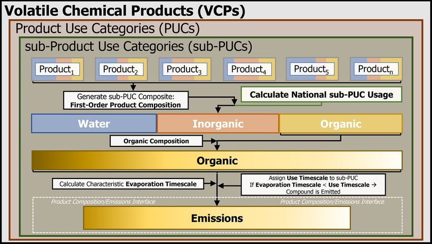
Figure 1. Conceptual overview of the VCPy framework. Note that PUC stands for product use category.
2 Methods ing quantitative structure–activity relationship (QSAR) mod-
eled physiochemical properties and compared to the assigned
2.1 VCPy: a framework for estimating reactive organic use timescale. If the characteristic evaporation timescale of
carbon emissions from volatile chemical products the organic component is less than the assigned use timescale
of the composite, it is assumed that the compound is emitted.
If not, the compound is retained in the product or other con-
The VCPy framework is based on the principle that the mag-
densed phase (e.g., water) and permanently sequestered.
nitude and speciation of organic emissions from VCPs are
directly related to (1) the mass of chemical products used,
(2) the composition of these products, (3) the physiochemical
properties of their constituents that govern volatilization, and 2.1.1 Product use categories (PUCs) and sub-product
(4) the timescale available for these constituents to evaporate use categories (sub-PUCs)
(Fig. 1). Since the VCP sector includes residential, commer-
cial, institutional, and industrial sources, a consistent stream
of data sources for all product categories is difficult. As such, VCPy disaggregates the VCP sector into several components
this work implements a hybridized methodology that utilizes called product use categories (PUCs). An individual PUC is
the best features of prior emission inventory methods, while not exclusively used in a singular setting (e.g., residential vs.
introducing new methods to make improvements where nec- commercial), and examples include personal care products,
essary. The result produces national-level per capita emis- cleaning products, and paints and coatings. PUCs are further
sion factors for all product categories in the VCP sector that divided into sub-PUCs, which are composites of individual
can be further tailored for regional or localized analysis. The product types featuring similar use patterns. In addition to
per capita basis is useful for comparison across frameworks permitting tailored fate and transport assumptions, similar hi-
and over time, but emissions can be recast in other units as erarchical product schema are also useful for models estimat-
needed. Briefly, survey data are used to generate a first-order ing near-field exposure to chemicals through routes such as
product composition profile for a composite of product types, dermal contact and indoor inhalation (Isaacs et al., 2020). As
which quantifies the fraction of organic, inorganic, and wa- an example, there are two sub-PUCs allocated to the personal
ter components. The organic component is further divided care product PUC: short-use products and daily use products.
into individual species (e.g., ethanol, isobutane, isopropyl al- These two sub-PUCs are differentiated by the length of use
cohol). A variety of data sources are used to estimate the prior to removal (i.e., the use timescale). The mass of chem-
national-level product usage, and each composite is assigned ical products used and subsequent organic emission factors,
a use timescale, reflecting the elapsed time between use and which are the main output from VCPy, are calculated at the
any explicit removal process. Finally, the characteristic evap- sub-PUC level (Fig. 1). Currently, there are 10 PUCs and 16
oration timescale of each organic component is calculated us- sub-PUCs implemented in VCPy (Table 1).
https://doi.org/10.5194/acp-21-5079-2021 Atmos. Chem. Phys., 21, 5079–5100, 2021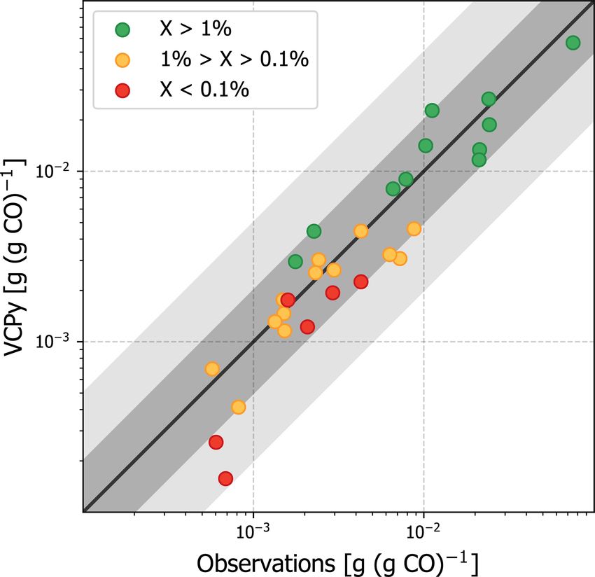
5082                                  K. M. Seltzer et al.: Reactive organic carbon emissions from volatile chemical products

Table 1. Description of all PUCs and sub-PUCs currently implemented in VCPy, their estimated mass usage for 2016, and product examples
of each. See Table S2 for a derivation of all product usage estimates.

  Product use         Sub-product use           2016 annual usage   Product examples
  categories          categories                   [kg per person
  (PUCs)              (sub-PUCs)                        per year]
  Cleaning products   Detergents and soaps                 40.58    Soaps, detergents, metal cleaners, scouring cleaners
                      General cleaners                     28.47    Disinfectants, air fresheners, glass and bathroom cleaners,
                                                                    windshield washer fluid, hand sanitizer, automotive and
                                                                    floor polishes, bleaches, surfactants
  Personal care       Daily use products                     8.83   Hair products, perfumes, colognes, cleansing and moisturizing creams,
  products                                                          sunscreens, hand and body lotion and oils, cosmetics, deodorants
                      Short-use products                     3.16   Shampoo, conditioners, shaving cream, aftershave,
                                                                    mouthwashes, toothpaste
  Adhesives and       Adhesives and sealants               15.23    Glues and adhesives, epoxy adhesives, other adhesives, structural
  sealants                                                          and nonstructural caulking compounds and sealants
  Paints and          Architectural coatings               13.27    Exterior/interior flat/gloss paints, primers, sealers, lacquers
  coatings            Aerosol coatings                       0.39   Paint concentrates produced for aerosol containers
                      Allied paint products                  1.26   Thinners, strippers, cleaners, paint/varnish removers
                      Industrial coatings                    7.42   Automotive, appliance, furniture, paper, electrical insulating, marine,
                                                                    maintenance, and traffic marking finishes and paints
  Printing inks       Printing inks                          3.20   Letterpress, lithographic, gravure, flexographic,
                                                                    non-impact/digital inks
  Pesticides and      FIFRA pesticides                       1.46   Lawn and garden pesticides and chemicals, household and
  FIFRA products                                                    institutional pesticides and chemicals
                      Agricultural pesticides              10.32    Agricultural and commercial pesticides and other organic chemicals
  Dry cleaning        Dry cleaning                           0.03   Dry cleaning fluids
  Oil and gas         Oil and gas                            1.32   Cleaners, deicers
  Misc. products      Misc. products                         0.18   Pens, markers, arts and crafts, dyes
  Fuels and lighter   Fuels and lighter                      2.80   Lighter fluid, fire starter, other fuels

2.1.2   National-level product usage                                    vey of Manufactures (ASM; U.S. Census Bureau, 2016a),
                                                                        which provides annual statistical estimates for all manufac-
                                                                        turing establishments. Values are available for all six-digit
To estimate VCP product use, some prior work has used na-               North American Industry Classification System (NAICS)
tional economic statistics, such as market sales or shipment            codes, provided as product shipment values (USD yr−1 ), and
values (e.g., U.S. Environmental Protection Agency, 2020;               are reported with associated relative standard errors (gener-
McDonald et al., 2018). Others have incorporated product                ally < 5 %). To translate shipment values (USD yr−1 ) to us-
usage statistics based on consumer habits and practices (e.g.,          age (kg yr−1 ), we use commodity prices (USD kg−1 ) from
Isaacs et al., 2014; Qin et al., 2020), but these statistics are        the U.S. Department of Transportation’s 2012 Commodity
generally unavailable for commercial and industrial chem-               Flow Survey (U.S. Department of Transportation, 2015). An
ical usage, which limits their application. To better ensure            exception is for all paint and coating sub-PUCs. Commod-
the capture of all chemical product usage, including usage in           ity prices for these sub-PUCs are taken from the U.S. Cen-
residential, commercial, institutional, and industrial settings,        sus Bureau’s Paint and Allied Products Survey (U.S. Census
where possible national economic statistics are utilized (Ta-           Bureau, 2011a) and are representative of 2010. To translate
ble S1 in the Supplement).                                              these commodity prices, which are from 2010 and 2012, to
   Product usage from 12 sub-PUCs is estimated using                    values reflective of 2016, we use producer price indices re-
national-level shipment statistics, commodity prices, and               ported by the Federal Reserve Bank of St. Louis (U.S. Bu-
producer price indices. National-level economic statistics              reau of Labor Statistics, 2020). Commodity price indices
are retrieved from the U.S. Census Bureau’s Annual Sur-

Atmos. Chem. Phys., 21, 5079–5100, 2021                                                       https://doi.org/10.5194/acp-21-5079-2021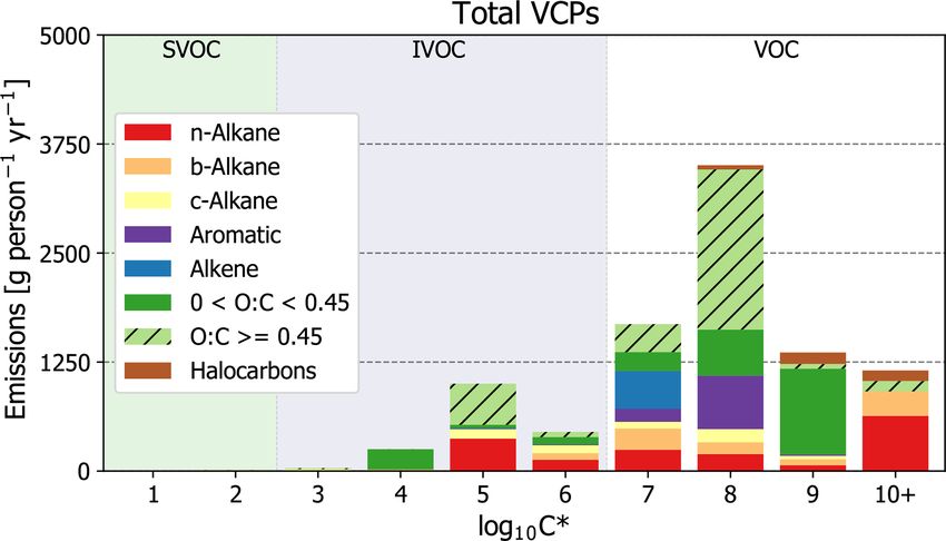
K. M. Seltzer et al.: Reactive organic carbon emissions from volatile chemical products                                      5083

from the Federal Reserve Bank are updated for all NAICS           order product composition profiles of industrial maintenance
manufacturing codes monthly, which we average to create           coatings and graphic arts coatings, respectively. The first-
annual price indices (Table S2). An implicit assumption in        order product composition profile for aerosol coatings uses
this methodology is that manufacturing and product usage          data from the California Air Resources Board’s 2010 Aerosol
are, on average, annually balanced.                               Coatings Survey (CARB, 2012), which includes more than
   We preferentially utilize product usage numbers derived        20 aerosolized product types. Only the evaporative organic
from the above methodology, when possible, as all data            composition of aerosol coating products was reported, so the
sources have the following characteristics: (1) they are na-      remaining mass was evenly split between water and inorgan-
tionally derived and therefore less influenced by regional        ics. For dry cleaning and oil and gas, as the product usage
differences in manufacturing and formulation, and (2) all         for these sub-PUCs was derived from the organic functional
datasets are freely available to the public. However, due to      solvent mass usage, it is assumed that this mass is entirely
data limitations, product usage for four sub-PUCs is esti-        evaporative organics.
mated using other sources. The dry cleaning and oil and gas          The second composite is the organic composition profile.
product usage estimates are derived from the national-level       Again, the California Air Resources Board’s 2015 Consumer
solvent mass usage reported by an industry study (The Free-       and Commercial Products Survey (CARB, 2019) was used
donia Group, 2016). The miscellaneous products and fuels          to derive a composite of product types for 10 sub-PUCs
and lighter product usage estimates are derived from reported     (Table S4). These product types are then mapped to an as-
sales data, specific to California, from the California Air Re-   sociated organic profile (CARB, 2018; see Table S3) and
sources Board’s 2015 Consumer and Commercial Products             weighted based on their evaporative organic contributions to
Survey Data (CARB, 2019). These sales numbers are scaled          the total sub-PUC. For architectural coatings, a 94 % water-
upwards to a national-level by assuming equivalent per capita     based and 6 % solvent-based paint (CARB, 2014) com-
product usage.                                                    posite is generated. Aerosol coatings are calculated on a
                                                                  weighted basis using the potentially evaporative organic con-
2.1.3   First-order and organic product composition               tributions reported by CARB’s 2010 Aerosol Coatings Sur-
                                                                  vey (CARB, 2012). The organic composition profiles for in-
Each sub-PUC features two composite profiles. The ini-            dustrial coatings, printing inks, and dry cleaning all utilize
tial composite is the first-order product composition profile,    profiles (3149, 2570, 2422, respectively) from EPA’s SPECI-
which disaggregates the total mass of each sub-PUC into           ATEv5.0 database (EPA, 2019b). Approximately 65 % of the
its water, inorganic, and organic fractions (Table 2). The or-    solvents used in the oil and gas sector are alcohols, and the
ganic component is further decomposed into non-evaporative        remainder are a broad range of hydrocarbons (The Freedonia
and evaporative organics. The quantification and accounting       Group, 2016). Since detailed composition data for oil and gas
of evaporative organics in this framework are necessary as        solvents are sparse, all oil and gas alcohols are assumed to
CARB’s organic profiles are processed to exclude organics         be methanol, as it is widely used in and emitted from oil and
that are not anticipated to evaporate on atmospherically rel-     gas operations (Lyman et al., 2018; Stringfellow et al., 2017;
evant timescales. For 10 sub-PUCs, the first-order product        Mansfield et al., 2018). The remaining 35 % is allocated to
composition profile uses data from the California Air Re-         naphtha, a blend of hydrocarbon solvents.
sources Board’s 2015 Consumer and Commercial Products                Several components within CARB profiles are lumped cat-
Survey (CARB, 2019). Various product types are sorted into        egories or complex mixtures. This includes naphtha, min-
each sub-PUC and the first-order product composition pro-         eral spirits, distillates, Stoddard solvent, fragrances, volatile
files are calculated on a weighted basis using the reported       methyl siloxanes, and a series of architectural coating and
sales from manufacturers and formulators in California. Due       consumer product “bins.” All naphtha, mineral spirits, distil-
to omissions stemming from confidentiality concerns, not all      lates, and Stoddard solvent occurrences in individual profiles
sales and composition data from the survey are available.         are treated as a single-mineral spirit profile (Carter, 2015).
We utilize the publicly available portions of the data, which     Volatile methyl siloxanes include several compounds (e.g.,
constitutes most of the survey and includes over 330 prod-        D4 , D5 , D6 ), all of which are emitted in varying proportions
uct types. For example, 126 product types and 20 product          (Janechek et al., 2017). Here, the lumped volatile methyl
types were sorted into the general cleaners and adhesives and     siloxane identity is preserved but the physiochemical prop-
sealants (Table S3) sub-PUCs, respectively.                       erties of decamethylcyclopentasiloxane is applied to the sur-
   For architectural coatings, industrial coatings, and print-    rogate. Fragrances are a diverse mixture of organic com-
ing inks, the first-order product composition profile is de-      pounds that include many terpenes and alkenes (Nazaroff and
rived from data in the California Air Resources Board’s 2005      Weschler, 2004; Sarwar et al., 2004; Singer et al., 2006b).
Architectural Coatings Survey (CARB, 2007). The Architec-         However, since the proportion of these constituents are un-
tural Coatings sub-PUC uses data from all profiles in the sur-    known, all fragrances are physically treated as d-limonene
vey, which is dominated by flat paint, non-flat paints, and       since it is the most prevalent terpene emitted from fragranced
primers. Industrial coatings and printing inks use the first-     products (Sarwar et al., 2004; Singer et al., 2006b). Finally,

https://doi.org/10.5194/acp-21-5079-2021                                           Atmos. Chem. Phys., 21, 5079–5100, 2021
5084 K. M. Seltzer et al.: Reactive organic carbon emissions from volatile chemical products
Table 2. First-order product composition profiles and evaporative organics proportion for all sub-PUCs.
Product use categories Sub-product use categories Water Inorganic Non-evaporative Evaporative
(PUCs) (sub-PUCs) [%] [%] organicsa organicsa
[%] [%]
Cleaning products Detergents and soapsb 67.8 13.9 15.4 2.9
General cleanersb 73.3 8.6 11.1 6.9
Personal care products Daily use productsb 48.8 10.7 16.9 23.7
Short-use productsb 72.2 5.8 17.7 4.3
Adhesives and sealants Adhesives and sealantsb 12.8 53.2 29.0 5.0
Paints and coatings Architectural coatingsc 45.5 49.6 0.0 5.0
Aerosol coatingsd 12.7 12.7 0.0 74.7
Allied paint productsb 5.1 3.5 0.6 90.8
Industrial coatingse 15.0 70.0 0.0 14.0
Printing inks Printing inksf 8.0 67.0 0.0 25.0
Pesticides and FIFRA products FIFRA pesticidesb 74.8 4.9 15.1 5.1
Agricultural pesticidesb 74.8 4.9 15.1 5.1
Dry cleaning Dry cleaningg 0.0 0.0 0.0 100
Oil and gas Oil and gasg 0.0 0.0 0.0 100
Misc. products Misc. productsb 27.1 14.6 48.8 9.5
Fuels and lighter Fuels and lighterb 0.0 92.9 0.0 7.1
a “Non-evaporative organics” and “evaporative organics” sum to total product organics. “Evaporative organics” represent the potentially evaporative organic
fraction of the total product and excludes assumed “non-evaporative” (i.e., assumed non-volatile) organics, which are not included in the California Air
Resource Board’s organic profiles. b California Air Resources Board 2015 Consumer and Commercial Products Survey Data (CARB, 2019). c California Air
Resources Board 2005 Architectural Coatings Survey (CARB, 2007). VOC + exempt is used for both organic and evaporative organics. Non-evaporative
organic proportions not provided. Sales proportions of water-based vs. solvent-based architectural coatings based on California Air Resource Board 2014
Architectural Coatings Survey (CARB, 2014). d California Air Resources Board 2010 Aerosol Coatings Survey (CARB, 2012); only evaporative organics is
provided; the remainder (∼ 25 %) is split evenly between water and inorganics. e Industrial maintenance composition data from California Air Resources
Board 2005 Architectural Coatings Survey (CARB, 2007). f Graphic Arts composition data from California Air Resources Board 2005 Architectural
Coatings Survey (CARB, 2007). g All product usage is composed of organic functional solvents (The Freedonia Group, 2016). Therefore, all mass is
assumed to be potentially evaporative.
for the architectural coating and consumer product “bins,” of the most stringent limits in the country (Ozone Transport
we use the representative chemical compositions derived by Commission, 2016). As the first-order and organic composi-
Carter, 2015. tion profiles utilized here are almost exclusively derived from
product composition data, pre-use controls are implicitly rep-
2.1.4 Controls resented. In fact, since the product composition data is from
manufacturers and formulators in California, where product
There are two methods for controlling organic emissions VOC content limits are typically more stringent than national
from VCPs. The first method is through product reformu- regulations, applying these profiles nationally likely results
lation, which would occur prior to product usage. Strategies in conservative assumptions.
that fit this definition include switching from a hydrocarbon The second pathway of controlling organic emissions from
solvent-based ingredient to one that is water-based, replac- VCPs is through post-use controls. Strategies that fit this def-
ing an organic component with a non-organic component, inition include add-on controls, manufacturing process mod-
and reformulating a product with lower-volatility ingredients ifications, and disposal techniques. Add-on control strategies
that are less likely to evaporate (Ozone Transport Commis- and manufacturing process modifications are limited to in-
sion, 2016). VCP emissions that stem from residential, com- dustrial and commercial emission sources, such as indus-
mercial, and institutional settings rely on these pre-use con- trial coating (U.S. EPA, 2007, 2008) and printing ink (U.S.
trols to reduce emissions. Regulators often set VOC content EPA, 2006a, b) facilities. Since adoption of these technolo-
limits for chemical products (e.g., national standards: Sec- gies vary widely in space and time, assigning post-use con-
tion 183(e) of the Clean Air Act; 40 CFR 59), with Cali- trols via these strategies is not considered here. As several
fornia (e.g., CARB – Title 17 CCR) typically setting some of these industrial sources (e.g., coatings, printing inks, dry
Atmos. Chem. Phys., 21, 5079–5100, 2021 https://doi.org/10.5194/acp-21-5079-2021K. M. Seltzer et al.: Reactive organic carbon emissions from volatile chemical products 5085
cleaning) feature controls, as required by Section 112 of the model OPERA (Mansouri et al., 2018) are used here. All
Clean Air Act (40 CFR 63), this assumption could lead to lo- physiochemical properties, including OPERA results, are re-
calized high bias and will be refined in future work. Here, we trieved from the U.S. EPA’s CompTox Chemistry Dashboard
only consider post-use controls through disposal techniques (https://comptox.epa.gov/dashboard, last access: 31 August
for the oil and gas and fuels and lighter sub-PUCs. For oil 2020).
and gas, we assume that the solvents used in these processes Use timescale is the timescale available for a sub-PUC to
become entrained in the produced water at these sites. Since evaporate and is based on the length of its direct use phase
produced water is largely (∼ 89 %–98 %) reinjected for en- (i.e., the elapsed time between application and any explicit
hanced oil and gas recovery or disposal (Lyman et al., 2018; removal process). As this value is subjective, broad values
Liden et al., 2018), we apply a post-use control efficiency of are applied to each sub-PUC (Table S5). For example, it
94 % (i.e., average of reported reinjection rates) to this sub- is assumed that all products used in the bath and shower
PUC. However, it should be noted that reinjection frequency are quickly sequestered and washed down the drain, thus
and solvent usage can vary regionally. For fuels and lighters, largely unavailable for emission (Shin et al., 2015). As such,
we assume 90 % of the organics are destroyed through com- short-use personal care products are assigned a “minutes”
bustion upon use (CARB, 2019). use timescale. In contrast, it is also assumed that each per-
son bathes once a day, and associated daily use personal care
2.1.5 Evaporation timescale and use timescale products are therefore assigned a “days” use timescale.
Emissions are determined by comparing the calculated
Fate and transport in the VCPy framework is a function of evaporation timescale for each component with the assigned
the predicted compound-specific evaporation timescale and use timescale for the sub-PUC. If the use timescale for the
the assigned use timescale of each sub-PUC. It should be sub-PUC is greater than the evaporation timescale for a com-
noted that this methodology explicitly results in the organic pound, the compound is emitted. Else, the compound is re-
speciation of emissions differing from the organic composi- tained in the product or other condensed phase and perma-
tion of products from which they volatilize. For example, the nently sequestered. Overall, organic emissions (E) for the
composition of organics within a product may differ from complete sector are calculated as a summation over all or-
the speciation of emitted organics if the product contains ganic compounds, i, and sub-PUCs, j , as follows:
low-volatility compounds that do not evaporate on relevant
timescales.
0
The evaporation timescale is the compound-specific (i.e.,
independent of the sub-PUC of interest) characteristic X if use timescalej < evaporation timescalei
E= (2)
timescale of emission from a surface layer and is calcu- U · f · f · (1 − f )
i,j j E j S i,j C j
lated using previously published methods (Khare and Gen-
if use timescale ≥ evaporation timescale ,
tner, 2018; Weschler and Nazaroff, 2008). This timescale is j i
defined as a relationship between the mass of a compound
applied and the rate of its emission, which can be expressed where U is the product usage (Table 1), fE is the evaporative
by organic fraction (Table 2), fS is the fraction of an organic
compound in the evaporative organics portion of a sub-PUC
Mapplied KOA · d (Table S4), and fC is the fraction of emissions that feature
Evaporation timescale [h] = = , (1) post-use controls on a mass basis. Application of Eq. (2) de-
Remission ve
termines the difference between organic product composition
where KOA is the octanol–air partitioning coefficient of the and organic emissions speciation.
compound, d [m] is the assumed depth of the applied prod-
uct layer, and ve [m h−1 ] is the mass transfer coefficient of 2.2 Uncertainty analysis
the compound from the surface layer into the bulk air, which
is a function of aerodynamic and boundary layer resistances. The sensitivity of emission estimates to a variety of input
Median values for d [0.1 mm] and ve [30 m h−1 ] from Khare variables are tested through a systematic Monte Carlo anal-
and Gentner (2018) are selected here. It should be noted ysis. We perform 10 000 simulations where product usage,
that ve can vary substantially based on outdoor vs. indoor evaporative organic proportions, variables associated with
atmospheric conditions, and future work will incorporate a the characteristic evaporation timescale, the assigned use
two-box model to better account for such differences. A com- timescale, and post-use control assumptions are tested, both
pound’s KOA is the ratio of an organic chemical’s concentra- individually and collectively. For product usage, the primary
tion in octanol to the organic chemical’s concentration in air sources of uncertainty are shipment values provided by the
at equilibrium. It is often used to quantify the partitioning be- ASM, commodity prices, the balance of imports (including
havior of an organic compound between air and a matrix. As tourism) and exports, and unused product disposal. The ASM
experimental values of KOA are sparse, modeled estimates provides standard error estimates for most shipment values,
from the quantitative structure–activity relationship (QSAR) which are typically less than 5 %. Uncertainty estimates are
https://doi.org/10.5194/acp-21-5079-2021 Atmos. Chem. Phys., 21, 5079–5100, 20215086 K. M. Seltzer et al.: Reactive organic carbon emissions from volatile chemical products
not provided for commodity prices, and national-level ex- sion, data in the County Business Patterns (CBP) is withheld
ports generally outweigh traditional imports for most sub- due to confidentiality concerns. In those instances, we take
PUCs (∼ 2 %–15 %; U.S. Census Bureau, 2016), but there the midpoint of the range associated with each data suppres-
are also imports of personal care products through tourism. sion flag. For agricultural pesticides, emissions are allocated
Therefore, we assume there is a ± 25 % uncertainty (95 % CI) based on county-level agricultural pesticide use and again
for all product usage estimates. CARB does not provide un- taken from the 2017 NEI (U.S. EPA, 2020). Oil and gas emis-
certainty estimates associated with the composition of prod- sions are allocated using oil and gas well counts (U.S. EIA,
uct types or sales proportions. To account for these uncer- 2019).
tainties, as well as the uncertainties associated with gener-
ating composites, we assume there is a ± 25 % uncertainty 2.4 Inventory evaluation
(95 % CI) for all “evaporative organic” (Table 2) proportions.
For the characteristic evaporation timescale, there are several Previously published emission ratios from the Los Ange-
layers of uncertainty. Application patterns vary by product les basin during the summer of 2010 (de Gouw et al.,
type, which impacts assumptions regarding the depth of the 2018, 2017) are used to evaluate the VCPy emissions in-
chemical layer. In addition, indoor vs. outdoor product use ventory (Table S7). Emissions ratios are generated by post-
and application of products to variable surface types (e.g., ab- processing observed concentrations of organic gases, typi-
sorbing vs. non-absorbing) can impact mass transfer rates. As cally normalized to carbon monoxide (CO) or acetylene, to
such, we apply broad uncertainties for variables associated a period of “no chemistry” (Borbon et al., 2013; de Gouw
with the characteristic evaporation timescale. We assume d et al., 2005; Warneke et al., 2007). As the air parcel is not
(i.e., the depth of the applied chemical layer) is lognormally photochemically aged (i.e., “no chemistry”), it is an ideal tool
distributed with a median value of 0.1 mm (95 % CI ∼ [0.01– for evaluating an emissions inventory. An important caveat is
1 mm]), and ve (i.e., the mass transfer coefficient) is normally that this method assumes the species being used for normal-
distributed with a mean value of 30 m h−1 (95 % CI = [10– ization (e.g., CO) is accurately inventoried and measured.
50 m h−1 ]). Since use timescales are categorical (e.g., min- Since the emission ratios are not specific to a sector and
utes, days, years), we apply uncertainty by assuming the represent total emissions, all other sectors must be quantified
95 % CI of the assigned use timescale features a ± 1 categor- and speciated. For this purpose, all non-VCP anthropogenic
ical uncertainty (e.g., mean: minutes; 95 % CI = [seconds – emissions from the 2017 NEI (U.S. EPA, 2020) are collected
hours]). Finally, for non-zero post-use controls, we assume and speciated using EPA’s SPECIATEv5.0 database (EPA,
a ± 25 % uncertainty (95 % CI) in the post-use control effi- 2019b; Table S8). This includes all on road, non-road, non-
ciency. It should be noted that additional avenues of uncer- point, and point sources. All VCP emissions from the 2017
tainty likely persist but are difficult to quantify and there- NEI are also collected and speciated for supplementary eval-
fore not included here. For example, due to the scarcity of uation. In addition, biogenic emissions of ethanol, methanol,
large-scale product surveys, many of the first-order prod- and acetone for May and June 2016, as simulated by the Bio-
uct composition profiles (e.g., architectural coatings) and or- genic Emission Inventory System (Bash et al., 2016), were
ganic profiles (e.g., printing inks) used in this analysis are included to capture non-anthropogenic sources of these com-
more than a decade old. As a result, the proportion of or- pounds. May and June were selected to coincide with the ob-
ganics in these product types and their organic components servational sampling months (de Gouw et al., 2018, 2017).
(i.e., the mean values applied here) may have changed in As the observed emission ratios are specific to the Los An-
the interim period. Furthermore, the uncertainty associated geles basin, we derive all VCPy inventory emission ratios
with the evaporative organic composition of individual prod- using data for Los Angeles County. Total CO emissions, in-
uct types is not known or provided by the source data. cluding all on-road, non-road, nonpoint, and point sources,
for Los Angeles County in 2017 are ∼ 320 Gg. While the
2.3 Spatial allocation of national-level emissions observed and VCPy inventory emission ratios are separated
by 6–7 years, the ambient non-methane hydrocarbon to CO
Emissions are calculated at the national-level and spatially concentration ratio in Los Angeles has been consistent for
allocated to the county-level using several proxies. A total of several decades, indicating changes in emission controls fea-
10 sub-PUCs, including all cleaning products and personal ture similar improvements for both pollutants over time (Mc-
care products, are allocated using population (Table S6; U.S. Donald et al., 2013). In addition, the magnitude of observed
Census Bureau, 2020). Four sub-PUCs (industrial coatings, emission ratios for a given region do not appreciably change
allied paint products, printing inks, dry cleaning), all typi- over marginal time horizons (Warneke et al., 2007).
cally industrial in nature, are allocated using county-level
employment statistics from the U.S. Census Bureau’s County 2.5 Air quality impact potential
Business Patterns (U.S. Census Bureau, 2018). The employ-
ment mapping scheme for these four sub-PUCs utilize the Each organic compound is assigned a SOA yield and max-
methods from the 2017 NEI (U.S. EPA, 2020). On occa- imum incremental reactivity (MIR) to facilitate an approx-
Atmos. Chem. Phys., 21, 5079–5100, 2021 https://doi.org/10.5194/acp-21-5079-2021K. M. Seltzer et al.: Reactive organic carbon emissions from volatile chemical products 5087
imation of the potential air quality impacts of VCPs. For
SOA, a wide collection of published yields, including both
chamber results and prediction tools, were utilized (Fig. S1
in the Supplement). These include (1) all linear alkanes use a
quadratic polynomial fit to the volatility basis set (VBS) data
from Presto et al. (2010) at 10 µg m−3 ; (2) all cyclic alka-
nes use linear alkane yields that are three carbons larger in
size (Tkacik et al., 2012); (3) all branched alkanes use yields
obtained from the Statistical Oxidation Model (SOM; Cappa
and Wilson, 2012), as reported in McDonald et al. (2018);
(4) benzene and xylenes use the average yields from Ng et al.
(2007) under high-NOx conditions; (5) toluene uses the aver-
age from Ng et al. (2007) under high-NOx conditions and the
Figure 2. Sector-wide volatility distribution of emissions by com-
VBS data from Hildebrant et al. (2009) at 10 µg m−3 ; (6) all pound class.
alkenes use yields obtained from SOM, as reported in Mc-
Donald et al. (2018); (7) volatile methyl siloxanes use the
two-product model parameters from Janecheck et al. (2019),
which includes additional SOA yields from Wu and Johnson is equal in magnitude to the sum of all mobile sources na-
(2017), at 10 µg m−3 ; (8) all glycol ethers use chamber results tionally, which is broadly consistent with the national-level
and molecular structure relationships from Li and Cocker emissions estimate from the 2017 NEI. Categorically, emis-
(2018) for reported and unreported glycol ethers, respec- sion factors are largest for paints and coatings, which total
tively; (9) benzyl alcohol uses the average of the lower-bound 3.1 kg per person per year (2.2 kg C per person per year) and
yields reported by Charan et al. (2020); (10) all remaining are approximately 33 % of the total sector (Table 3). The next
non-cyclic oxygenates, where available, use the arithmetic largest PUCs are personal care products and cleaning prod-
average of SOM results and a 1-D VBS approach, as reported ucts, which contribute 2.1 kg per person per year (22 %) and
by McDonald et al. (2018); (11) all remaining cyclic oxy- 2.0 kg per person per year (21 %), respectively. Printing inks,
genates, where available, use yields obtained from SOM, as adhesives and sealants, and pesticides each account for 6 %–
reported by McDonald et al. (2018); (12) all halocarbons and 9 % each, and the remaining PUCs contribute less than 2 %
compounds with less than five carbons are assigned a yield in total.
of zero; and (13) all remaining species are conservatively as- For the complete sector (Fig. 2), the most abundantly
signed a yield of zero if the effective saturation concentra- emitted compound classes were oxygenated species (53 %),
tion (i.e., C ∗ = (P vap ·MW)/(R·T )) is ≥ 3 × 10⁶ µg m−3 and followed by alkanes (31 %; including straight-chained,
assigned the same yield as n-dodecane if the effective satu- branched, and cyclic), aromatics (8 %), alkenes (5 %), and
ration concentration is < 3 × 10⁶ µg m−3 . The MIR of each halocarbons (3 %). Individually, organic emissions are dom-
compound, which measures the formation potential of ozone inated by ethanol (daily use products, general cleaners), ace-
under various atmospheric conditions where ozone is sensi- tone (paints and coatings, general cleaners), isopropyl alco-
tive to changes in organic compounds (Carter, 2010b), is cal- hol (daily use products, general cleaners), toluene (paints
culated using the SAPRC-07 chemical mechanism (Carter, and coatings, adhesives and sealants), n-tetradecane (print-
2010a) and expressed as a mass of additional ozone formed ing inks), fragrances (daily use products, general clean-
per mass of organic emitted (Carter, 2010b). ers), propane (aerosol coatings, industrial coatings), and
volatile methyl siloxanes (daily use products, adhesives and
sealants). Each of these species compose > 3 % of total VCP
3 Results and discussion organic emissions (see Table S9 for the top 200 most emitted
compounds).
3.1 National-level PUC and sub-PUC emissions In terms of volatility classification (Donahue et al.,
2012), as determined by the effective saturation con-
National-level, per capita organic emissions from VCPs are centration (i.e., C∗ ), total emissions are predominately
9.5 kg per person per year (6.4 kg C per person per year) VOCs (C ∗ > 3 × 10⁶ µg m−3 ), but there are also con-
for 2016 (Table 3), which translates to 3.05 Tg (2.06 Tg C). siderable contributions from IVOCs (3 × 10² µg m−3 <
When filtered to remove regulatory exempt organics, total C ∗ < 3 × 10⁶ µg m−3 ; Figs. 2 and 3). IVOC emissions, which
emissions from VCPs are 2.6 Tg of VOC. In comparison, the are efficient SOA precursors (Chan et al., 2009; Presto et al.,
2017 NEI reports a combined total of 2.6 Tg of VOC emis- 2010), are approximately 20 % of total emissions. Of the
sions for on-road mobile, non-road mobile, and other mobile 20 % that are IVOCs, 52 % are oxygenated compounds (e.g.,
(i.e., aircraft, commercial marine vessels, and locomotives) Texanol™, propylene glycol, ethylene glycol, siloxanes, ben-
sources. Therefore, when measured as VOC, the VCP sector zyl alcohol, and glycol ethers), 30 % are n-alkanes, and the
https://doi.org/10.5194/acp-21-5079-2021 Atmos. Chem. Phys., 21, 5079–5100, 20215088 K. M. Seltzer et al.: Reactive organic carbon emissions from volatile chemical products
Table 3. National-level emissions, volatilization fraction, and proportion of all usage that is emitted for all sub-PUCs.
Product use Sub-product use ROC Organic Total product
categories categories emissions volatilization emitted
(PUCs) (sub-PUCs) fraction [%]a [%]
[kg per person [kg C per person
per year] per year]
Cleaning products Detergents and soaps 0.12 0.06 1.6 0.3
General cleaners 1.85 1.25 36.0 6.5
Personal care products Daily use products 2.04 1.12 56.9 23.1
Short-use products 0.02 0.01 3.3 0.7
Adhesives and sealants Adhesives and sealants 0.76 0.56 14.7 5.0
Paints and coatings Architectural coatings 0.67 0.37 100b 5.0
Aerosol coatings 0.29 0.22 100b 74.7
Allied paint products 1.14 0.80 99.2 90.6
Industrial coatings 1.04 0.79 100b 14.0
Printing inks Printing inks 0.80 0.65 100b 25.0
Pesticides and FIFRA FIFRA pesticides 0.07 0.06 25.2 5.1
products Agricultural pesticides 0.53 0.41 25.2 5.1
Dry cleaning Dry cleaning 0.01 0.01 34.5 34.5
Oil and gas Oil and gas 0.08 0.04 6.0 6.0
Misc. products Misc. products 0.02 0.01 16.3 9.5
Fuels and lighter Fuels and lighter 0.02 0.02 10.0 0.7
Total 9.45 6.38 31.5 6.9
a Volatilization fraction represents the fraction of the total organic content of products that volatilize and emit to ambient air. b The “organic” portion of these
sub-PUCs is entirely composed of “evaporative organics” (see Table 2). Only data from the California Air Resources Board’s 2015 Consumer and Commercial
Products Survey featured the disaggregation of evaporative and non-evaporative organics. Prior surveys typically combined the non-evaporative organic
portion of each profile with solids or inorganics.
rest are largely branched and cyclic alkanes. The promi- but 40.6 % of daily use products are organic while general
nence of oxygenated IVOC emissions from VCPs is note- cleaners are overwhelming composed of water (Table 2), and
worthy, as SOA yields from these compounds have not his- the annual mass usage of general cleaners is ∼ 3× higher
torically been evaluated or included as SOA precursors in than daily use products (Table 1). As a result, net emis-
model chemical mechanisms (Qin et al., 2020). However, sions of general cleaners are within 10 % of those from daily
work has been undertaken in recent years to better under- use products (1.85 and 2.04 kg per person per year, respec-
stand these compounds (e.g., Wu and Johnson, 2017; Li and tively). The emissions of short-use products, which is as-
Cocker, 2018; Janechek et al., 2019; Charan et al., 2020). signed a “minutes” use timescale, can further illustrate the
Overall, paints and coatings is the largest source of IVOC importance of considering fate and transport. Under these use
emissions (∼ 760 g per person per year; Fig. 3), followed by timescale assumptions, only high-volatility compounds (i.e.,
printing inks (∼ 350 g per person per year), cleaning prod- C ∗ > 3 × 10⁷ µg m−3 ) are emitted and a majority (∼ 97 %) of
ucts (∼ 180 g per person per year), and pesticides (∼ 170 g its organics are retained (Table 3). Besides daily use products
per person per year). While paints and coatings emit more and general cleaners, all remaining sub-PUCs emit ≤ 1.14 kg
IVOCs by mass than all other PUCs, printing ink and pesti- per person per year, with six emitting less than 0.1 kg per per-
cide emissions both feature greater proportions of IVOCs to son per year (Table 3). Generally, sub-PUCs with low emis-
their total emissions (∼ 44 % and ∼ 28 %, respectively). sions stem from minimal use (e.g., misc. products), short-use
These results also highlight how emissions from each PUC timescales (e.g., short-use products), or high control assump-
and sub-PUC are uniquely driven by the mass of products tions (e.g., oil and gas, fuels and lighter).
used, organic composition, and use timescale. For example,
the two largest sub-PUC sources are daily use products and
general cleaners. Both are assigned a use timescale of 24 h,
Atmos. Chem. Phys., 21, 5079–5100, 2021 https://doi.org/10.5194/acp-21-5079-2021K. M. Seltzer et al.: Reactive organic carbon emissions from volatile chemical products 5089
Figure 3. PUC and sector-wide volatility distribution of organic emissions. Other is a summation of dry cleaning, oil and gas, misc. products,
and fuels and lighter. Pie charts are first-order product composition and organic emission proportions for PUCs and the complete sector. Note
that the “organic” portion of all paints and coatings and printing inks pie charts is entirely composed of “evaporative organics” (see Table 2).
3.2 Uncertainty analysis of national-level emission in a total sector-wide emission uncertainty of ± 15 % (Fig. 4;
factors 9.5 kg per person per year, 95 % CI: 8.1–10.9). Interestingly,
the interaction of evaporation and use timescales can result
Uncertainty associated with product usage, proportion of in a threshold effect, where small changes in either do not
evaporative organics, assumptions related to evaporation and necessarily translate into changes in the magnitude of emis-
use timescale, and post-use controls, where applicable, result sions for a given sub-PUC (Fig. S2). For many PUCs, such
https://doi.org/10.5194/acp-21-5079-2021 Atmos. Chem. Phys., 21, 5079–5100, 20215090 K. M. Seltzer et al.: Reactive organic carbon emissions from volatile chemical products
Figure 4. Monte Carlo sensitivity results for organic emissions. (a) Mean, interquartile range, and 95 % confidence intervals for six PUCs
and a combination of the remaining four (dry cleaning, oil and gas, misc. products, and fuels and lighter). (b) Probability distribution of
sector-wide emission estimates. See Table S10 for a tabulation of this figure.
as paints and coatings, adhesives and sealants, and printing half the emissions magnitude reported elsewhere (McDonald
inks, the use timescale is sufficiently long (i.e., years) for et al., 2018).
all evaporative organics to evaporate, regardless of the un-
certainty associated with the evaporation and use timescales. 3.3 State- and county-level emissions allocation
Under such conditions, only uncertainty in product usage and
product composition affect uncertainty in the emission mag-
The magnitude of VCP emissions varies substantially
nitude. As a result, these two variables are the largest drivers
throughout the country, with the most populated states and
of uncertainty for the complete sector (Fig. S2). However, un-
counties featuring the highest ROC emissions (Fig. 5). Cal-
certainties associated with evaporation and use timescale as-
ifornia (349 Gg), Texas (247 Gg), and Florida (173 Gg) are
sumptions can be important for certain sub-PUCs with mod-
the largest state-level emitters and contribute ∼ 25 % of all
erate to low use timescales (see cleaning products in Fig. S2).
VCP emissions. In contrast, the 30 smallest state-level emit-
For example, detergents and soaps is assigned a “minutes”
ters (plus Washington, D.C.) together emit ∼ 780 Gg. At the
use timescale, which results in a 0.12 kg per person per year
county-level, Los Angeles County, Cook County (Chicago),
emission factor (Table 3). If the use timescale for this sub-
and Harris County (Houston) are the largest emitters. How-
PUC was changed “hours,” the emission factor would in-
ever, after normalizing by population, these three counties
crease by a factor of 5.
all feature per capita emissions (8.21, 8.88, and 8.76 kg per
From a national emissions perspective, these Monte Carlo
person per year, respectively) less than the national average
results contain several important results. First, as mentioned
(9.45 kg per person per year) due to less industrial activity.
above, the largest drivers of uncertainty are associated with
National spatial variability in per capita emissions are
a sub-PUC’s usage and composition, not assumptions related
largely driven by sub-PUCs tied to industrial and commer-
to fate and transport (i.e., evaporation and use timescales).
cial activity (Fig. 5c). These sub-PUCs include allied paint
Second, the most uncertain PUCs are cleaning products, per-
products (1.14 kg per person per year), industrial coatings
sonal care products, and paints and coatings, and their un-
(1.04 kg per person per year), printing inks (0.80 kg per per-
certainty generates a significant amount of emissions poten-
son per year), agricultural pesticides (0.53 kg per person
tial. The 95 % confidence interval for all three span > 1.24 kg
per year), and oil and gas (0.08 kg per person per year).
per person per year, which is equivalent to > 400 Gg of or-
The employment proxies for allied paint products, indus-
ganic emissions per year. Finally, the 95 % confidence inter-
trial coatings, and printing inks are usually consistent with
val for the national-level emissions from the complete sector
the underlying population (Fig. S3), with peaks in Califor-
for 2016 is 2.6–3.5 Tg (1.8–2.4 Tg C), which is broadly con-
nia, Texas, Florida, New York, and the industrial Midwest.
sistent with the U.S. EPA’s 2017 NEI (2.8 Tg) and, largely
In contrast, emissions from agricultural pesticides and oil
due to differences in predicted evaporation, approximately
and gas drive the large per capita emissions in the Midwest
Atmos. Chem. Phys., 21, 5079–5100, 2021 https://doi.org/10.5194/acp-21-5079-2021K. M. Seltzer et al.: Reactive organic carbon emissions from volatile chemical products 5091
emissions, respectively. Both sub-PUCs also contribute to
atypically high per capita emissions in other states, such as
Texas, Colorado, Idaho, and Wyoming.
While national VCP emissions from the 2017 NEI and the
VCPy inventory are broadly consistent, county-level and cat-
egorical estimates can differ substantially between the two
(Fig. S4). For example, VCPy reports > 35 % lower emis-
sions for 5 % of all counties and > 55 % higher emissions
for another 5 % of all counties. When compared to the 2017
NEI, the states with the greatest emissions increases were
Delaware, California, and Colorado, and the states with the
greatest emissions decreases were North Dakota and South
Dakota. There are also many spatial similarities between the
two inventories. Both feature peaks in per capita emissions
over the Midwest and Great Plains (Fig. S4), and approx-
imately half of all county-level emissions in the VCPy in-
ventory are within 15 % of their value in the 2017 NEI.
To compare the two inventories categorically, all product
use categories are mapped to individual source classification
codes (SCCs; Table S11). Categorically, VCPy reports higher
emissions for personal care products (150 %) and paints and
coatings (25 %), whereas pesticides (−54 %) and printing
inks (−13 %) feature emission decreases. The VCPy inven-
tory also includes marginal increases in cleaning products
and adhesives and sealants emissions, while also quantifying
solvent-borne emissions in oil and gas operations (included
as “other” in Fig. S5).
3.4 Evaluation of inventory using emission ratios
Predicted per capita VCP emissions in Los Angeles County
are 8.21 kg per person per year and consist of 250+ organic
compounds. Observed emission ratios were available for 30
species (Table S7), including some of the most abundantly
emitted (e.g., ethanol, acetone, isopropyl alcohol, toluene).
In fact, of the 30 available emission ratios, 24 were for
compounds that contributed more than 0.1 % to total VCP
emissions (Fig. 6), providing the opportunity to evaluate im-
portant markers. For most compounds, the VCPy estimate
was well within a factor of 2 when compared to obser-
vations. Some important markers were marginally low bi-
ased (e.g., ethanol, isopropyl alcohol), while others were
marginally high biased (e.g., acetone, methyl ethyl ketone,
isobutane), illustrating the difficulty in precisely speciating
organic emissions and uncertainties introduced by composit-
Figure 5. (a) State-level, (b) county-level, and (c) county-level per ing. However, when considered as a whole, the complete
capita VCP emissions. VCPy inventory performs remarkably well with a correlation
of 0.95. In total, the observed emission ratio for all 30 com-
pounds was 0.259 g (g CO)−1 and the inventory estimate is
and Great Plains (Fig. 5c). Emissions from these two sub- 0.226 g (g CO)−1 , indicating a 13 % low bias. In addition, the
PUCs are heavily concentrated in the central United States VCPy inventory shows a marked improvement over the 2017
(Fig. S3), including North Dakota, South Dakota, Iowa, Ne- NEI, which reports 3.28 kg per person per year of VCP emis-
braska, Kansas, and Oklahoma. Collectively, these states sions in Los Angeles County. For the 30 compounds consid-
contain < 4.5 % of the United States population but 24.1 % ered here, the 2017 NEI reports 0.143 g (g CO)−1 , which is
and 17.5 % of the agricultural pesticides and oil and gas VCP 45 % lower than observations (Fig. S6). Most notably, the
https://doi.org/10.5194/acp-21-5079-2021 Atmos. Chem. Phys., 21, 5079–5100, 2021You can also read