An ensemble square root filter for the joint assimilation of surface soil moisture and leaf area index within the Land Data Assimilation System ...
←
→
Page content transcription
If your browser does not render page correctly, please read the page content below
Hydrol. Earth Syst. Sci., 24, 325–347, 2020
https://doi.org/10.5194/hess-24-325-2020
© Author(s) 2020. This work is distributed under
the Creative Commons Attribution 4.0 License.

An ensemble square root filter for the joint assimilation of surface
soil moisture and leaf area index within the Land Data Assimilation
System LDAS-Monde: application over the Euro-Mediterranean
region
Bertrand Bonan1 , Clément Albergel1 , Yongjun Zheng1 , Alina Lavinia Barbu1 , David Fairbairn2 , Simon Munier1 , and
Jean-Christophe Calvet1
1 CNRM,   Université de Toulouse, Météo-France, CNRS, Toulouse, France
2 European Centre for Medium-Range Weather Forecasts, Reading, UK

Correspondence: Clément Albergel (clement.albergel@meteo.fr)

Received: 26 July 2019 – Discussion started: 20 August 2019
Revised: 19 November 2019 – Accepted: 7 December 2019 – Published: 23 January 2020

Abstract. This paper introduces an ensemble square root           SSM and soil moisture in deeper soil layers is found, as ex-
filter (EnSRF) in the context of jointly assimilating ob-         pected, showing seasonal patterns that vary geographically.
servations of surface soil moisture (SSM) and the leaf            Moderate correlation and anti-correlations are also noticed
area index (LAI) in the Land Data Assimilation System             between LAI and soil moisture, varying in space and time.
LDAS-Monde. By ingesting those satellite-derived products,        Their absolute value, reaching their maximum in summer
LDAS-Monde constrains the Interaction between Soil, Bio-          and their minimum in winter, tends to be larger for soil mois-
sphere and Atmosphere (ISBA) land surface model (LSM),            ture in root-zone areas, showing that assimilating LAI can
coupled with the CNRM (Centre National de Recherches              have an influence on soil moisture. Finally an independent
Météorologiques) version of the Total Runoff Integrating          evaluation of both assimilation approaches is conducted us-
Pathways (CTRIP) model to improve the reanalysis of land          ing satellite estimates of evapotranspiration (ET) and gross
surface variables (LSVs). To evaluate its ability to produce      primary production (GPP) as well as measures of river dis-
improved LSVs reanalyses, the EnSRF is compared with the          charges from gauging stations. The EnSRF shows a system-
simplified extended Kalman filter (SEKF), which has been          atic albeit moderate improvement of root mean square dif-
well studied within the LDAS-Monde framework. The com-            ferences (RMSDs) and correlations for ET and GPP prod-
parison is carried out over the Euro-Mediterranean region at      ucts, but its main improvement is observed on river dis-
a 0.25◦ spatial resolution between 2008 and 2017. Both data       charges with a high positive impact on Nash–Sutcliffe effi-
assimilation approaches provide a positive impact on SSM          ciency scores. Compared to the EnSRF, the SEKF displays a
and LAI estimates with respect to the model alone, putting        more contrasting performance.
them closer to assimilated observations. The SEKF and the
EnSRF have a similar behaviour for LAI showing perfor-
mance levels that are influenced by the vegetation type. For
SSM, EnSRF estimates tend to be closer to observations than       1   Introduction
SEKF values. The comparison between the two data assimi-
lation approaches is also carried out on unobserved soil mois-    Land surface variables (LSVs) are key components of the
ture in the other layers of soil. Unobserved control variables    Earth’s water, vegetation and carbon cycles. Understand-
are updated in the EnSRF through covariances and correla-         ing their behaviour and simulating their evolution is a chal-
tions sampled from the ensemble linking them to observed          lenging task that has significant implications on various
control variables. In our context, a strong correlation between   topics, from vegetation monitoring to weather prediction

Published by Copernicus Publications on behalf of the European Geosciences Union.
326                                                                           B. Bonan et al.: An ensemble square root filter

and climate change (Bonan, 2008; Dirmeyer et al., 2015;            2019, among others) and particle filters (see e.g. Pan et al.,
Schellekens et al., 2017). Land surface models (LSMs) play         2008; Plaza et al., 2012; Zhang et al., 2017; Berg et al.,
an important role in improving our knowledge of land surface       2019) for estimating soil moisture profiles. Those various ap-
processes and their interactions with the other components of      proaches have been extensively compared in the context of
the climate system such as the atmosphere. Forced by atmo-         the sole assimilation of soil moisture retrievals (Reichle et
spheric data and coupled with river routing models, they aim       al., 2002; Sabater et al., 2007; Fairbairn et al., 2015).
to simulate LSVs such as soil moisture (SM), biomass and              LDASs are, however, not restricted to soil moisture. Re-
the leaf area index (LAI). However, LSMs are prone to errors       cently, monitoring vegetation dynamics through LDASs has
owing to inaccurate initialization, misspecified parameters,       gained attention. LAI is a key land biophysical variable; it is
flawed forcing or inadequate model physics. Another way to         defined as half the total area of green elements of the canopy
monitor LSVs is to use observations either from in situ net-       per unit horizontal ground area. One way to monitor LAI is to
works or satellites. While in situ networks generally provide      assimilate observations already used for surface soil moisture
sparse spatial coverage, remote sensing provides global cov-       and indirectly linked to LAI, such as the brightness temper-
erage of LSVs at spatial resolutions ranging from the kilo-        ature for low microwave frequencies (see e.g. Vreugdenhil
metre scale to the metre scale but at a daily frequency at best    et al., 2016) and radar backscatter coefficient (Lievens et al.,
(Lettenmaier et al., 2015; Balsamo et al., 2018). Not all key      2017; Shamambo et al., 2019, among others). This is the ap-
LSVs are observed directly from space. For example, passive        proach followed by Sawada et al. (2015) and Sawada (2018),
microwave satellite sensors used traditionally to estimate soil    who assimilate brightness temperatures using a particle fil-
moisture are sensible only to the near-surface (0–2 cm depth)      ter to jointly estimate soil moisture profiles and LAI in the
moisture content (Schmugge, 1983), leading to the develop-         Coupled Land Vegetation LDAS (CLVLDAS).
ment of indirect approaches to estimate root-zone soil mois-          Another way to constrain LAI is through the assimila-
ture from satellite data (see e.g. Albergel et al., 2008).         tion of direct LAI observations in LDASs. Satellite-derived
   Combining observations with LSMs can overcome flaws             LAI products benefit from recent advances in remote sens-
in both approaches. This is the objective of Land Data As-         ing (Fang et al., 2013; Baret et al., 2013; Xiao et al., 2013),
similation Systems (LDASs). Many of them focus on assim-           and datasets are now available at the global scale and at high
ilating observations related to surface soil moisture (SSM),       resolution. While other studies have assimilated LAI in crop
either using passive microwave brightness temperatures, mi-        models and at a more local scale (see e.g. Pauwels et al.,
crowave backscatter coefficients or soil moisture retrievals       2007; Ines et al., 2013; Jin et al., 2018), such assimilation has
obtained from the aforementioned satellite observations, to        been, to our knowledge, seldom performed by LDASs. Jar-
estimate soil moisture profiles (Lahoz and De Lannoy, 2014;        lan et al. (2008) and Sabater et al. (2008) have succeeded in
Reichle et al., 2014; De Lannoy et al., 2016; Maggioni et          introducing such an approach in LDASs. The latter study has
al., 2017, and references therein). One popular approach has       notably shown that jointly assimilating observations of SSM
been the simplified extended Kalman filter (SEKF). Intro-          and LAI can improve the quality of root-zone SM estimates
duced at Météo-France by Mahfouf et al. (2009), it was ini-        for one location in southwestern France. This work has been
tially designed for assimilating screen level observations to      carried out with the CO2 -responsive version of the Interac-
correct soil moisture estimates in the context of numerical        tions between Soil, Biosphere and Atmosphere (ISBA) LSM
weather prediction and is now involved in the operational          (Calvet et al., 1998, 2004; Gibelin et al., 2006), developed by
systems of both the European Centre for Medium-Range               CNRM (Centre National de Recherches Météorologiques).
Weather Forecast (ECMWF; Drusch et al., 2009; de Ros-              This version of ISBA allows for the simulation of vegetation
nay et al., 2013) and the UK Met Office. The SEKF has              dynamics including biomass and LAI. Building on that work,
also been applied to the sole assimilation of soil moisture        Albergel et al. (2010), Rüdiger et al. (2010) and Barbu et al.
retrievals (Draper et al., 2009) and then to the joint assim-      (2011) introduced a SEKF jointly assimilating SSM and LAI
ilation of soil moisture retrievals and leaf area indices (Al-     and tested the approach on the SMOSREX (Surface Monitor-
bergel et al., 2010; Barbu et al., 2011). Even though the          ing Of the Soil Reservoir EXperiment) site located in south-
SEKF approach has provided good results, it suffers from           western France. Their study has been extended to a series of
several limitations. It relies on a climatological background      locations over France (Dewaele et al., 2017) and to France
error covariance matrix assuming uncorrelated variables be-        (Barbu et al., 2014; Fairbairn et al., 2017) leading to the de-
tween grid points and involves the computation of a Jaco-          velopment of the LDAS-Monde (Albergel et al., 2017). The
bian matrix to build covariances between control variables at      LDAS-Monde suite is available through the CNRM mod-
the same location. This Jacobian matrix is computed with fi-       elling platform SURFEX (SURFace EXternalisée; Masson
nite differences, meaning that one model run is required per       et al., 2013) and it has been successfully applied to various
control variable, thus limiting the size of the control vector.    parts of the globe: Europe and the Mediterranean basin (Al-
That is why SEKF has been in competition with more flexi-          bergel et al., 2017, 2019; Leroux et al., 2018), the contiguous
ble approaches, such as the ensemble Kalman filter (EnKF)          United States (Albergel et al., 2018b), and Burkina Faso (Tall
(Reichle et al., 2002; Fairbairn et al., 2015; Blyverket et al.,   et al., 2019).

Hydrol. Earth Syst. Sci., 24, 325–347, 2020                                       www.hydrol-earth-syst-sci.net/24/325/2020/
B. Bonan et al.: An ensemble square root filter                                                                               327

   Lately other LDASs have started assimilating LAI using             – and assimilating satellite-derived soil water index (SWI;
an EnKF assimilation approach. For example, Fox et al.                  as a proxy for SSM) and LAI products from the Coper-
(2018) assimilated LAI and biomass in order to reconstruct              nicus Global Land Service (CGLS).
the vegetation and carbon cycles for a site in Mexico, while
Ling et al. (2019) compared various approaches for the as-        The performance of both data assimilation (DA) approaches
similation of LAI at a global scale. In addition Kumar et al.     is assessed with (i) satellite-driven model estimates of land
(2019) assimilated LAI with an EnKF in the North Amer-            evapotranspiration (ET) from the Global Land Evaporation
ican Land Data Assimilation System phase 2 (NLDAS-2)              Amsterdam Model (GLEAM, Miralles et al., 2011; Martens
and studied its impact not only on vegetation but also on soil    et al., 2017), (ii) upscaled ground-based observations of gross
moisture, with those LSVs being updated indirectly through        primary production (GPP) from the FLUXCOM project (Tra-
the model using the updated LAI. These studies did not up-        montana et al., 2016; Jung et al., 2017) and (iii) river dis-
date both SM and LAI, as we will do in this study.                charges from the Global Runoff Data Centre (GRDC). The
   This paper aims to develop an EnKF approach for the            paper is organized as follows: Sect. 2 details the various com-
joint assimilation of LAI and SSM in the LDAS-Monde.              ponents involved in LDAS-Monde including the data assim-
To that end, it will build upon the work of Fairbairn et al.      ilation schemes. Section 3 describes the experimental setup
(2015), which introduced an ensemble square root filter (En-      and the different datasets used in the experiment such as at-
SRF; Whitaker and Hamill, 2002) in the LDAS-Monde in              mospheric forcing or assimilated observations. Section 3 also
the context of assimilating SSM alone. The EnSRF is one of        details the datasets used to assess the performance of the En-
the many deterministic formulations of the EnKF (see e.g.         SRF and the SEKF. The impact of the EnSRF on LSVs is
Tippett et al., 2003; Livings et al., 2008; Sakov and Oke,        then assessed in Sect. 4, including the comparison with the
2008). Fairbairn et al. (2015) compared the performance of        SEKF. Finally, the paper discusses the issues encountered
the EnSRF with the SEKF, routinely used in the LDAS-              during the experiment and provides prospects for future work
Monde, over 12 sites in southwestern France. While perform-       in Sect. 5, before concluding in Sect. 6.
ing better on synthetic experiments, the EnSRF provides re-
sults that are equivalent to the SEKF for real cases. Related
                                                                  2     LDAS-Monde
to that work, Blyverket et al. (2019) used another determin-
istic EnKF to assimilate satellite-derived SSM values from        LDAS-Monde is the offline, global-scale and sequential-
the Soil Moisture Active Passive (SMAP) satellite over the        data-assimilation system dedicated to land surfaces devel-
contiguous United States with the ISBA LSM. This work fo-         oped by the Météo-France research centre, CNRM (Albergel
cused on soil moisture in the near surface, while it did not      et al., 2017). Embedded within the open-access SURFEX
update root-zone soil moisture directly through data assimi-      surface modelling platform (Masson et al., 2013; https://
lation.                                                           www.umr-cnrm.fr/surfex/, last access: 16 January 2020), it
   The present paper aims to (1) adapt the EnSRF to the           consists of the ISBA land surface model coupled with the
joint assimilation of LAI and SSM within the LDAS-Monde,          CTRIP river routing system and data assimilation. Those
(2) study the impact of assimilating LAI and SSM on LSVs          routines routinely assimilate satellite-based products of SSM
using an ensemble approach, and (3) compare the EnSRF             and LAI to analyse and update soil moisture and LAI mod-
with the routinely used SEKF and its ability to provide im-       elled by ISBA. The most recent SURFEX v8.1 implemen-
proved LSV estimates. To achieve these goals, LDAS-Monde          tation is used in our experiments. We quickly recall the
with EnSRF and SEKF is applied to the Euro-Mediterranean          main components of LDAS-Monde and subsequently de-
region for a 10-year experiment (from 2008 to 2017):              tail the novel EnSRF approach for the joint assimilation of
                                                                  SSM and LAI. More information can be found in Albergel
  – using the vegetation interactive ISBA-A-gs (CO2 -             et al. (2017) (see also https://www.umr-cnrm.fr/spip.php?
    responsive version of the ISBA LSM) LSM (Calvet et            article1022&lang=en, last access: 16 January 2020).
    al., 1998, 2004; Gibelin et al., 2006) with the multi-layer
    soil diffusion scheme from Decharme et al. (2011),            2.1    ISBA land surface model

                                                                  The ISBA LSM aims to simulate the evolution of LSVs such
  – coupled daily with CNRM version of the Total Runoff
                                                                  as soil moisture, soil heat or biomass (Noilhan and Planton,
    Integrating Pathways (CTRIP) river routing model
                                                                  1989; Noilhan and Mahfouf, 1996). In this paper we use the
    (Decharme et al., 2019) to simulate hydrological vari-
                                                                  ISBA multilayer diffusion scheme which solves the mixed
    ables such as river discharge,
                                                                  form of the Richards equation (Richards, 1931) for water and
                                                                  the one-dimensional Fourier law for heat (Boone et al., 2000;
  – forced by the latest ERA5 atmospheric reanalysis from         Decharme et al., 2011). The soil is discretized in 14 layers
    ECMWF (Hersbach and Dee, 2016; Hersbach et al.,               over a depth of 12 m. The lower boundary of each layer is
    2020),                                                        0.01, 0.04, 0.1, 0.2, 0.4, 0.6, 0.8, 1.0, 1.5, 2.0, 3.0, 5.0, 8.0

www.hydrol-earth-syst-sci.net/24/325/2020/                                        Hydrol. Earth Syst. Sci., 24, 325–347, 2020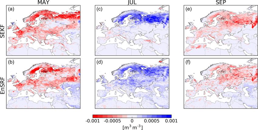
328                                                                               B. Bonan et al.: An ensemble square root filter

and 12 m depth (see Fig. 1. of Decharme et al., 2013). The        2.3     Data assimilation
chosen discretization minimizes the errors from the numeri-
cal approximation of the diffusion equations.                     LDAS-Monde is a sequential data assimilation system with a
   Regarding vegetation dynamics and interactions between         24 h assimilation window. Each cycle is divided in two steps:
the water and carbon cycles, we use the ISBA-A-gs config-         forecast and analysis. Quantities produced during the fore-
uration (Calvet et al., 1998, 2004; Gibelin et al., 2006). This   cast step (analysis step) are denoted with a superscript f (su-
CO2 -responsive version represents the relationship between       perscript a ). The state of the studied system is described by
the leaf-level net photosynthesis rate (A) and stomatal aper-     x [p] , the control vector that contains every prognostic vari-
ture (gs). Dynamics of vegetation variables such as LAI or        able of the ISBA LSM for a patch p and a given grid point.
biomass are induced by photosynthesis in response to atmo-        In this paper, we consider LAI and soil moisture from lay-
spheric variations. The LAI growing phase from a prescribed       ers 2 (1–4 cm depth; SM2) to 7 (60–80 cm depth; SM7) in
threshold (1.0 m2 m−2 for coniferous trees, 0.3 m2 m−2 for        the control vector, with soil moisture in layer 1 being driven
every other type of vegetation) results from an enhanced pho-     mostly by atmospheric forcings (Draper et al., 2011; Barbu et
tosynthesis and CO2 uptake. On the contrary, a deficit of pho-    al., 2014). As in many LDASs, LDAS-Monde performs DA
tosynthesis leads to higher mortality rates and a decreased       for each grid point independently (no spatial covariances are
LAI. Leaf biomass is determined from LAI (and vice versa)         considered).
through dividing LAI by the specific leaf area (one of the            The forecast step consists of propagating the state of the
ISBA parameters depending on the vegetation type). For arc-       system from a time t to t + 24 h using ISBA. Patches in each
tic regions, hydraulic and thermal soil properties are modi-      ISBA grid cell do not interact between each other. This im-
fied in order to include a dependency on soil organic carbon      plies that, for a patch p, the forecast of x [p] , denoted by
content (Decharme et al., 2016).                                  x f[p] (t + 24 h), only depends on the analysis at time t, x a[p] (t)
   From a practical point of view, ISBA is run in this pa-        and the ISBA LSM using the parametrization for patch p,
per at a regular 0.25◦ spatial resolution. Each ISBA grid cell    denoted by M[p] . This yields
is divided into 12 generic patches: nine representing differ-
ent types of vegetation (deciduous forests, coniferous forests,   x f[p] (t + 24 h) = M[p] x a[p] (t) .                            (1)
evergreen forests, C3 crops, C4 crops, C4 irrigated crops,
grasslands, tropical herbaceous and wetlands) and three oth-      The analysis step then corrects forecast estimates by assimi-
ers depicting bare soils, bare rocks and permanent snow or        lating observations of LAI and SSM.
ice surfaces. Each patch covers a varying percentage of grid
cells. Denoted α[p] for patch p of a given grid cell, this per-   2.3.1    Simplified extended Kalman filter
centage is also known as the patch fraction. Vegetation and
soil parameters for each ISBA patch and grid cell are derived     LDAS-Monde routinely uses a simplified extended Kalman
from the ECOCLIMAP II land cover database (Faroux et al.,         filter for the analysis step (Mahfouf et al., 2009). Observa-
2013), which is fully integrated in SURFEX.                       tions (SSM and/or LAI) are interpolated on the ISBA grid
                                                                  for assimilation (see Sect. 3.2 for more information). For
2.2   CTRIP river routing model                                   each ISBA grid cell, we consider the vector y o containing
                                                                  all the observations available for that grid cell at the time of
The ISBA LSM is coupled with CTRIP to simulate hy-                assimilation. The SEKF analysis step is in two parts. First we
drological variables at a continental scale. Based originally     calculate the model equivalent, denoted by y f , at the ISBA
on the work of Oki and Sud (1998), CTRIP aims to con-             grid cell level. This is performed by aggregating control vari-
vert simulated runoff into simulated river discharges. The        ables from each patch of the ISBA grid cell using a weighted
model is fully described in the following papers: Decharme        average.
et al. (2010), Decharme et al. (2012), Vergnes and Decharme
(2012), Vergnes et al. (2014), and Decharme et al. (2019).                12
                                                                          X
   CTRIP is available at a 0.5◦ spatial resolution. The cou-      yf =          α[k] Hx f[k] ,                                     (2)
pling between ISBA and CTRIP occurs on a daily basis                      k=1

through the OASIS3-MCT coupler (Model Coupling Toolkit            where H denotes the linear operator selecting model equiva-
of the OASIS coupler) (Voldoire et al., 2017). ISBA pro-          lent from each patch (modelled LAI for observed LAI; mod-
vides updated runoff, drainage, groundwater and floodplain        elled soil moisture in layer 2 for SSM).
recharges to CTRIP, while the river routing model returns            Then, the SEKF analysis step is performed for each ISBA
the water table depth or rise, floodplain fraction, and flood     grid cell. We further assume that there are no covariances
potential infiltration to the LSM.                                between the patches. Therefore, each patch is updated sepa-
                                                                  rately. For each patch, the SEKF analysis follows the tradi-
                                                                  tional Kalman update. It replaces the forecast error covari-
                                                                  ance matrix with a fixed prescribed error covariance matrix

Hydrol. Earth Syst. Sci., 24, 325–347, 2020                                            www.hydrol-earth-syst-sci.net/24/325/2020/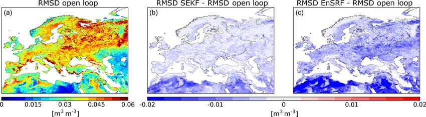
B. Bonan et al.: An ensemble square root filter                                                                                 329

B. The observation operator is the product of the model state        To that end, we first calculate the model equivalent of the ob-
evolution from t to t + 24 h and the conversion of the model         servations by aggregating the mean of the forecast ensemble
state into the observation equivalent. Thus, the Jacobian of         over all the patches.
the observation operator involves H and M[p] , the Jacobian
                                                                            12
matrix of M[p] . In the end, for each patch p, we have                      X
                                                                     yf =         α[k] Hx f[k]                                   (8)
                                 T                                       k=1
x a[p] = x f[p] + α[p] B HM[p]        C−1    o
                                       SEKF y − y
                                                  f
                                                              (3)
                                                                     The analysis step then updates the ensemble whose analysed
and                                                                  mean and covariance matrix exactly matches the analysis of
                                                                     the Kalman filter when the observation operator is linear.
            12
            X
                    2
                                    T                                  We choose to neglect the ensemble covariances between
CSEKF =            α[k] HM[k] B HM[k] + R,                    (4)    patches in the analysis step of the EnSRF. This assumption is
            k=1
                                                                     in line with the SEKF method, and it ensures a fair compari-
where R is the observation error covariance matrix. In prac-         son between the two approaches. The approach outlined here
tice, columns of M[p] are calculated by finite differences us-       is in line with other studies (Fairbairn et al., 2015; Carrera
ing perturbed model runs. For each component xj of the con-          et al., 2015) showing that 1-D EnKFs can achieve promising
trol vector and its perturbation δxj , the j th column of M[p]       results with around 20 ensemble members.
can be written as                                                        Following this assumption, for a given patch p, the anal-
                                                                     ysed mean and perturbation matrix are given by the following
        ∂x f (t + 24 h)                                            equations:
 M[p] j =
                ∂xj
                                                                     x a[p] = x f[p] + α[p] Pf[p] HT C−1      y o
                                                                                                                  − y f
                                                                                                                                (9)
             M[p] x a (t) + δxj − x f (t + 24 h)

                                                                                                      EnSRF
           ≈                                     .            (5)
                            δxj                                      and
Details on how to obtain Eqs. (3) and (4) can be found in the        Xa[p] = I − α[p] K
                                                                                      e[p] H Xf

                                                                                                                                (10)
                                                                                              [p]
Supplement.
                                                                     with
2.3.2     Ensemble square root filter
                                                                                   12
                                                                                   X
                                                                                          2
We adapt the EnSRF from Whitaker and Hamill (2002) to                CEnSRF =            α[k] HPf[k] HT + R                     (11)
the context of LDAS-Monde following the work of Fair-                              k=1
bairn et al. (2015). The EnSRF is an EnKF-based approach             and
in which the state of a system and associated uncertain-
                                                                                              −1/2                 −1
ties
n are described oby an ensemble of Ne control vectors

                                                                     e[p] = α[p] Pf HT CT              1/2       1/2
    (i)
                                                                     K            [p]   EnSRF        C EnSRF + R         . (12)
  x [p] , i = 1, . . ., Ne for patch p of a given grid cell.The
EnKF approximates the classical Kalman filter equations us-          Such an approach, contrary to the SEKF, updates the state
ing the ensemble mean                                                covariance matrix that will evolve in time. This ensures that
                                                                     information from the analysis is stored in the ensemble and
          Ne
          X      (i)                                                 is propagated forward in time.
x [p] =         x [p]                                         (6)
          i=1
                                                                     3     Experimental setup and datasets
to describe the state of the system and the ensemble covari-
ance matrix                                                          We detail in the following subsections the atmospheric forc-
           1                                                         ing, the assimilated observations and the validation datasets
P[p] =         X[p] XT[p] ,                                    (7)   employed in this paper before detailing the experimental
        Ne − 1
                                                                     setup.
               h                                  i
                  (1)                 (N )
where X[p] = x [p] − x [p] , . . ., x [p]e − x [p] is the ensemble   3.1    Atmospheric forcing
perturbation matrix used to describe the uncertainties of the
estimation.                                                          The ISBA LSM is forced with the ERA5 atmospheric re-
   In the forecast step, we propagate, as in Eq. (1), each en-       analysis (Hersbach and Dee, 2016; Hersbach et al., 2020)
semble member from time t to t + 24 h using the ISBA LSM.            developed by ECMWF. The ERA5 reanalysis is available
The analysis step then corrects the ensemble mean and the            with an hourly frequency at a 31 km horizontal spatial res-
ensemble perturbation matrix by assimilating observations.           olution. To be used, surface atmospheric variables such as

www.hydrol-earth-syst-sci.net/24/325/2020/                                               Hydrol. Earth Syst. Sci., 24, 325–347, 2020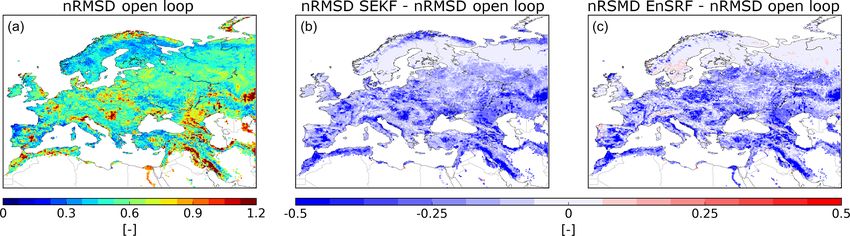
330 B. Bonan et al.: An ensemble square root filter
air temperature, surface pressure, solid and liquid precipita- 3.3 Validation datasets
tions, incoming shortwave and longwave radiations values,
and wind speed are interpolated to a 0.25◦ spatial resolu- We consider independent datasets of evapotranspiration
tion using bilinear interpolation. Replacing ECMWF’s atmo- (ET), gross primary production (GPP) and river discharges
spheric ERA-Interim reanalysis with ERA5 has been shown to assess the validity of our approach and measure the influ-
to be beneficial in the context of LSV reanalyses with LDASs ence of the EnSRF on the improvement of LSV reanalyses.
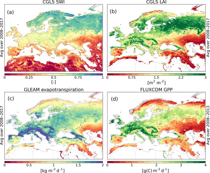
(Albergel et al., 2018a, b). Satellite-derived estimates of ET come from the GLEAM
v3.3b product (Miralles et al., 2011; Martens et al., 2017).
3.2 Observations for assimilation Daily estimates available for the period 1980–2018 at a 0.25◦
spatial resolution are fully driven by satellite observations
In this paper we assimilate observations from the SWI-001 and, as such, are independent of LDAS-Monde estimates.
and GEOLAND2 version 1 (GEOV1) LAI datasets, both Figure 1c displays GLEAM ET averaged over the period
being distributed by the Copernicus Global Land Service. 2008–2017 considered for validation in this paper.
These satellite-derived products have already been success- Observations of GPP are derived from the FLUXCOM
fully assimilated into LDAS-Monde (e.g. Leroux et al., 2018; project. This dataset is obtained by merging upscaled mea-
Albergel et al., 2019). surements from eddy-covariance flux towers and satellite
The SWI-001 product consists of soil water indices ob- observations using machine learning. More details can be
tained through a recursive exponential filter (Albergel et al., found in Tramontana et al. (2016) and Jung et al. (2017). The
2008) using backscatter observations from the ASCAT (Ad- FLUXCOM data are available at a 0.5◦ spatial resolution on
vanced SCATterometer) C-band radar (Wagner et al., 1999; a monthly basis for the period 1982–2013. Figure 1d shows
Bartalis et al., 2007). A 1 d timescale is used in the recursive FLUXCOM GPP averaged over the period 2008–2013 con-
filter in order to estimate the wetness of the first centimetres sidered for validation in this paper.
of the soil. This product is available daily at a 0.1◦ spatial River discharge output data from the CTRIP river routing
resolution. The raw SWI-001 averaged over the 2008–2017 model are compared to daily streamflow data obtained from
period can be seen in Fig. 1a. the Global Runoff Data Centre (https://www.bafg.de/GRDC,
Prior to the assimilation, the SWI-001 product needs to be last access: 16 January 2020). Due to the low resolution
rescaled to the model climatology to avoid introducing any of CTRIP (0.5◦ spatial resolution), we only consider data
bias in the LDAS system (Reichle and Koster, 2004; Drusch for sub-basins with rather large drainage areas (greater than
et al., 2005). We apply a linear rescaling to SWI-001 to match 10 000 km2 ) with a long enough time series (4 complete
the observation mean and variance to the mean and variance years or more over 2008–2017).
of the modelled soil moisture in the second layer of soil (1–
4 cm). Introduced by Scipal et al. (2008), this rescaling gives 3.4 Experimental setup
in practice very similar results to CDF (cumulative distribu-
tion function) matching. The linear rescaling is performed on To assess the impact of EnSRF on LSV reanalyses and
a seasonal basis (with a 3-month moving window). Draper et compare its skill with the routinely used SEKF, we have
al. (2009) and Barbu et al. (2014) have highlighted the im- run LDAS-Monde over the Euro-Mediterranean region (lon-
portance of allowing seasonal variability in the rescaling. gitude from 11.5◦ W to 62.5◦ E, latitude from 25.0◦ N to
The GEOLAND2 version 1 LAI product is obtained 75.5◦ N) at a 0.25◦ spatial resolution during the decade 2008–
through a neural network algorithm (Baret et al., 2013) trans- 2017 for three different configurations: one model run with-
forming observations of reflectance from SPOT-VGT and out assimilation (i.e. open loop), one using the SEKF and
PROBA-V satellites into LAI. This dataset is available ev- another one using the EnSRF with a 20-member ensemble.
ery 10 d with the finest spatial resolution being 1 km. The This size of the ensemble is consistent with Fairbairn et al.
GEOV1 LAI averaged over the 2008–2017 period can be (2015) and Carrera et al. (2015). All three configurations start
seen in Fig. 1b. from the same initial state obtained after spinning up ISBA–
Following Barbu et al. (2014), both observation datasets CTRIP 20 times over 2008. This provides an initial state for
are interpolated on the model grid (0.25◦ spatial resolution) which the system has reached equilibrium.
where and when at least half of the observation grid points For the SEKF configuration, the Jacobian matrix Eq. (5)
are available. As in previous LDAS-Monde studies, we use is obtained by finite differences using perturbed model runs.
a 24 h assimilation window, and observations are assimilated Following Draper et al. (2009) and subsequent studies, per-
at 09:00 UTC. turbations are taken proportional to the dynamic range (dif-
ference between the volumetric field capacity wfc and the
wilting point wwilt ) for the soil moisture variable. In prac-
tice, perturbations for SM are set to 10−4 ×(wfc − wwilt ). Re-
garding the fixed background error covariance, we prescribe
a mean volumetric standard deviation (SD) of 0.04 m3 m−3
Hydrol. Earth Syst. Sci., 24, 325–347, 2020 www.hydrol-earth-syst-sci.net/24/325/2020/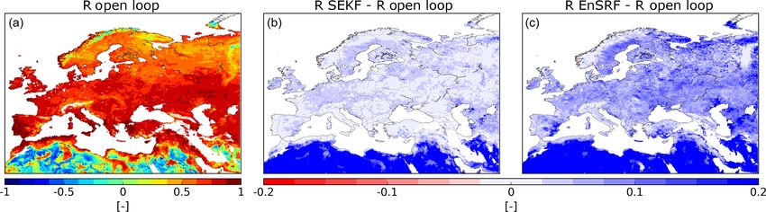
B. Bonan et al.: An ensemble square root filter                                                                                       331

Figure 1. Satellite-derived products of the (a) original soil water index (SWI), (b) leaf area index (LAI), (c) evapotranspiration (ET) and
(d) gross primary production (GPP) values. They are averaged over 2008–2017 for (a), (b) and (c) and over 2008–2013 for (d).

for SM in the second layer and 0.02 m3 m−3 for SM in deeper             model. We prescribe an associated Gaussian noise with zero
layers, both are then scaled by the dynamic range of SM. For            mean and an SD of λ (wfc − wwilt ) for SM, with λ = 0.5 for
LAI, perturbations are set to a fraction (0.001) of the mod-            SM in layer 2 (1–4 cm depth), 0.2 for SM in layer 3 (4–10 cm
elled LAI following Rüdiger et al. (2010). LAI background               depth), 0.05 for SM in layer 4 (10–20 cm depth) and 0.02 for
error SD is set to 20 % of the LAI value for modelled val-              SM in deeper layers. These values are in line with Fairbairn
ues above 2.0 m2 m−2 and to a constant 0.4 m2 m−2 for mod-              et al. (2015). For LAI, we prescribe a Gaussian noise with
elled values below 2.0 m2 m−2 . This SEKF configuration is              zero mean and an SD of 0.5 m2 −2 . We also fix the time cor-
the same as the one detailed in Albergel et al. (2017).                 relation to 1 d for SM in the second layer and 3 d for SM in
   About the EnSRF configuration, the initial ensemble is ob-           deeper layers. This is similar to the work of Reichle et al.
tained by perturbing the initial state using perturbations sam-         (2002) and Mahfouf (2007). For LAI, a rather small 1-day
pled from a multivariate Gaussian distribution with a zero              time correlation has to be used in order to avoid a collapse of
mean and using the prescribed B covariance matrix used in               the ensemble during the winter season due to the LAI thresh-
the SEKF as the covariance matrix of that multivariate Gaus-            old in ISBA.
sian distribution. Ensemble Kalman filters tend to underes-                For both SEKF and EnSRF configurations, we follow pre-
timate variances and ensembles spreads. This brings about               vious LDAS-Monde studies and set SSM observational er-
an artificially small spread leading ultimately to filter diver-        rors to 0.05 m3 m−3 scaled to the dynamic range and LAI ob-
gence if not counteracted. Hamill and Whitaker (2005) has               servational errors to 20 % of the observed LAI values (see e.g
shown that adding random perturbations to each ensemble                 Albergel et al., 2017; Leroux et al., 2018; Tall et al., 2019).
member (additive inflation) at the start of each assimilation
cycle can overcome this issue. It can also be used to repre-            3.5   Evaluation strategy
sent model error. As in Fairbairn et al. (2015) we use time-
correlated model errors using a first-order auto-regressive             As a check, we first verify that EnSRF estimates of SSM and
                                                                        LAI are closer to observations than their open-loop counter-

www.hydrol-earth-syst-sci.net/24/325/2020/                                               Hydrol. Earth Syst. Sci., 24, 325–347, 2020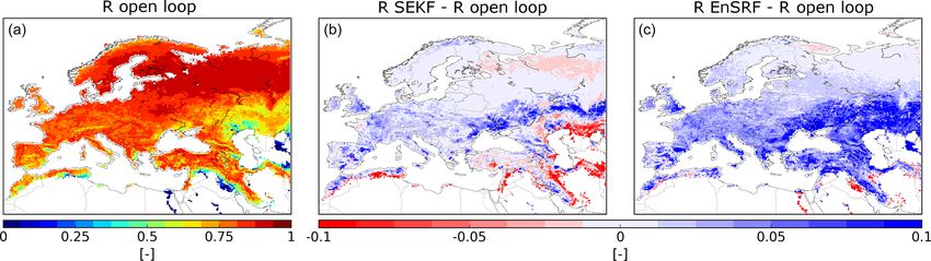
332                                                                          B. Bonan et al.: An ensemble square root filter

parts. We also compare the impact of EnSRF and SEKF on            vations. Both DA systems efficiently correct model simula-
SM in layer 2 (1–4 cm depth; SM2) and LAI. This is achieved       tions for that latter phase. However, both SEKF and EnSRF
using scores such as biases, correlation coefficients (R), root   fail to compensate for the slower LAI dynamics of the model
mean square differences (RMSDs) and normalized root mean          during spring. This is in compliance with what Albergel et
square differences (nRMSDs; RMSD divided by the aver-             al. (2017) and Leroux et al. (2018) have observed over the
aged value of the studied variable).                              Euro-Mediterranean region. During the growing phase, mod-
   The impact of assimilation on unobserved control vari-         elled LAI is more sensitive to atmospheric conditions than to
ables (SM in deeper layers) is then assessed using a daily        initial LAI conditions. This implies that, while DA can ar-
analysis increment. Moreover, we study the evolution of           tificially add LAI and biomass, its impact can be limited by
the ensemble correlations between unobserved and observed         the atmospheric forcing. During the senescence, LAI dynam-
variables in the EnSRF configuration. They drive (as Jaco-        ics is driven by the rate of mortality, thus making DA more
bian values in the SEKF configuration) the influence of ob-       efficient.
servations on unobserved control variables. We focus on SM            As expected, both DA approaches produce estimates
in layer 4 (10–20 cm depth; SM4) and layer 6 (40–60 cm            that are closer to the assimilated LAI observations than
depth; SM6), as SM in layer 3 (4–10 cm depth) exhibits the        their open-loop counterpart. RMSDs are reduced from
same behaviour as SM4, and soil moisture in layer 5 (20–          0.880 m2 m−2 for the open loop to 0.671 m2 m−2 for SEKF
40 cm depth) and layer 7 (60–80 cm depth) have the same           and 0.694 m2 m−2 for EnSRF. Correlations with assimilated
behaviour as SM6 (not shown).                                     observations are increased from 0.593 for the model to 0.732
   Potential improvements in EnSRF and SEKF estimates of          for SEKF and 0.723 for EnSRF. A full summary of statistics
ET and GPP are measured using the same metrics as for SSM         for LAI can be found in Table 1. We also note that the maxi-
and LAI.                                                          mum LAI for EnSRF is smaller than the model or the SEKF
   Finally the influence on river discharges for both DA ap-      maxima. The averaged bias for the open loop is rather small
proaches is measured by the Nash–Sutcliffe efficiency (NSE)       with −0.020 m2 m−2 , but it hides a negative bias during win-
score.                                                            ter and summer that is compensated for by a positive bias
             PT                                                   during autumn. DA approaches mostly correct the positive
                   (Qst − Qot )2                                  autumnal bias, thus making the averaged bias more negative,
NSE = 1 − Pt=1               o 2,                          (13)
                T     ot
                t=1 (Q − Q )
                                                                  −0.116 m2 m−2 for the SEKF and −0.201 m2 m−2 for the
                                                                  EnSRF. The bias is more negative for the EnSRF than for the
where Qst is the simulated or analysed river discharge at time    SEKF for every season. This is due in part to a systematic
                                                             o
t, Qot is the observed river discharge at the same time and Q     negative bias introduced by the EnSRF model perturbations.
is the observed averaged river discharge. The NSE is a quan-      This bias can sometimes lead to degraded performances. As
tity between −∞ and 1. An NSE value of 1 means that the           pointed out by Fairbairn et al. (2015), model perturbations
model or analysis perfectly matches observations. An NSE          can introduce a bias into the system in LDASs.
value of 0 means that the model or analysis has the same NSE          Figure 3 shows nRMSD calculated over 2008–2017 for
as the observed averaged river discharge. Improvements or         the open loop (a) and the difference between nRMSD for
degradations caused by the SEKF or the EnSRF compared to          the open loop and the estimates produced with SEKF (b)
the open loop is measured with the normalized information         and EnSRF (c). On average nRMSD is reduced from 0.57
contribution index (NIC).                                         (open loop) to 0.42 (EnSRF) and 0.40 (SEKF). Both as-
                                                                  similation approaches display the same geographical pat-
                  NSEanalysis − NSEmodel
NICNSE = 100 ×                                            (14)    terns significantly reducing nRMSD over most parts of the
                     1 − NSEmodel                                 Euro-Mediterranean region (in blue in Fig. 3). For example,
                                                                  roughly 20 % of the domain has an nRMSD reduced by 0.25.
4     Results                                                     We note that the largest nRMSD reductions occur in places
                                                                  where nRMSD is large. The main differences between the
4.1    Impact of assimilation on LAI                              two methods occur in Ireland, western Great Britain, north-
                                                                  west Spain, the Alps, Scandinavia and Arctic regions, where
Figure 2 displays the open-loop, SEKF and EnSRF analyses          the SEKF shows a greater positive impact than EnSRF, the
and observed LAI 10 d time series averaged over Europe and        latter even providing slightly degraded estimates compared
the Mediterranean basin and spanning the period 2008–2017.        to the open loop for 3 % of the total domain (in red in Fig. 3c).
It shows that the model simulation underestimates LAI com-            The geographical patterns identified in Fig. 3 can be ex-
pared to observations during winter and summer. The grow-         plained in part by the type of vegetation covering grid cells.
ing phase of vegetation occurs at a slower pace with averaged     We investigate the impact of DA for each of the four main
LAI reaching its maximum early August instead of late June        vegetation types encountered in the Euro-Mediterranean re-
to early July for observations. The senescence phase subse-       gion: deciduous forests, coniferous forests, C3 crops and
quently takes place later in the autumn compared to obser-        grasslands. To that end, we consider only grid cells (GCs) in

Hydrol. Earth Syst. Sci., 24, 325–347, 2020                                      www.hydrol-earth-syst-sci.net/24/325/2020/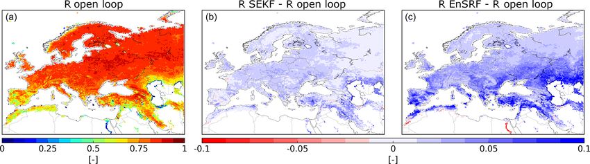
B. Bonan et al.: An ensemble square root filter                                                                                      333

Figure 2. 10 d time series of LAI averaged over the whole domain from the open loop (blue line), observations (green dots and dotted line)
and analyses obtained with the SEKF (dashed purple line) and the EnSRF (red line) for the period 2008–2017.

Table 1. Statistics (RMSD: root mean square difference, nRMSD: normalized RMSD, R: correlation and bias) between LDAS-Monde
estimates (open loop, SEKF and EnSRF) and observations for CGLS SSM, CGLS LAI, GLEAM ET and FLUXCOM GPP averaged over
the Euro-Mediterranean region for the period 2008–2017 (for SSM, LAI and ET) or 2008–2013 (for GPP).

                      Variable    Experiment     RMSD                   nRMSD          R                      Bias
                                  open loop      0.880 m2 m−2              0.568    0.593         −0.020 m2 m−2
                      LAI         SEKF           0.671 m2 m−2              0.401    0.732         −0.116 m2 m−2
                                  EnSRF          0.694 m2 m−2              0.419    0.723         −0.201 m2 m−2
                                  open loop      0.035 m3 m−3              0.161    0.544           0.002 m3 m−3
                      SSM         SEKF           0.032 m3 m−3              0.138    0.652           0.001 m3 m−3
                                  EnSRF          0.027 m3 m−3              0.117    0.760           0.001 m3 m−3
                                  open loop      0.833 kg m−2 d−1          0.712    0.789      −0.328 kg m−2 d−1
                      ET          SEKF           0.778 kg m−2 d−1          0.689    0.803      −0.114 kg m−2 d−1
                                  EnSRF          0.745 kg m−2 d−1          0.678    0.823      −0.059 kg m−2 d−1
                                  open loop      1.369 g(C) m−2 d−1        0.913    0.784    −0.412 g(C) m−2 d−1
                      GPP         SEKF           1.393 g(C) m−2 d−1        0.962    0.786    −0.146 g(C) m−2 d−1
                                  EnSRF          1.344 g(C) m−2 d−1        0.908    0.817    −0.105 g(C) m−2 d−1

which at least 50 % of their surface is covered by one of these        (Fig. 5d) as RMSDs are decreased by 0.18 m2 m−2 from the
vegetation types. Figure 4 displays the spatial distribution           open-loop to SEKF estimates but by 0.09 m2 m−2 for EnSRF
of those grid cells: 1589 GCs for deciduous forests (5.7 %             estimates. The largest RMSD reductions occur for both cases
of the domain), 4223 GCs for coniferous forests (15.2 %),              in April and September. This explains the reduced perfor-
1672 GCs for C3 crops (6.0 %) and 1725 GCs for grass-                  mance of the EnSRF compared to the SEKF over grasslands-
lands (6.2 %). We calculate the averaged seasonal RMSD                 dominated Ireland, western Great Britain and Arctic regions.
for the open loop and SEKF and EnSRF analyses for the                  For coniferous trees (Fig. 5b), the SEKF has a small positive
entire domain (Fig. 5a) and for each dominant vegetation               impact on RMSDs, and the EnSRF has a slightly negative
type (Fig. 5b–e). The biggest impact of assimilating LAI oc-           impact. This explains the rather poor performance of the En-
curs in autumn for deciduous forests (Fig. 5e). For exam-              SRF over Scandinavia. This also explains what happens in
ple, RMSD is reduced from 2.69 m2 m−2 for the open loop                northwestern Spain and in the Alps. While not being domi-
to 1.72 m2 m−2 for the SEKF and 1.45 m2 m−2 for the En-                nated by one type of vegetation, coniferous trees and grass-
SRF. For C3 crops (Fig. 5c) both assimilation approaches re-           lands, the two types for which the EnSRF performs poorly,
duce RMSD in a similar manner, the largest decrease hap-               represent more than 70 % of the vegetation in those places.
pening between August and October. The SEKF and the En-                   The scale of reduction in RMSD for EnSRF analyses is
SRF offer contrasting performances in the case of grasslands           directly connected to estimated variances and standard devi-

www.hydrol-earth-syst-sci.net/24/325/2020/                                              Hydrol. Earth Syst. Sci., 24, 325–347, 2020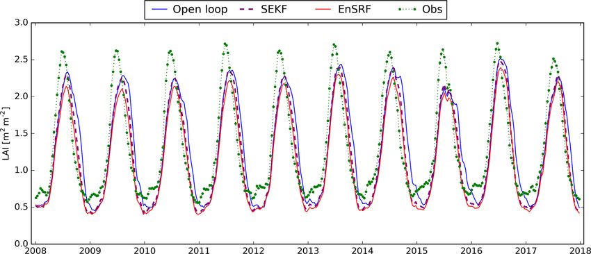
334                                                                              B. Bonan et al.: An ensemble square root filter

Figure 3. (a) Normalized RMSD (nRMSD) between observed LAI and its open-loop equivalent for the period 2008–2017 and the nRMSD
difference between assimilation experiments (SEKF in b and EnSRF in c) and the open loop.

                                                                      the same distribution. However, the behaviour of ensemble
                                                                      standard deviations varies greatly seasonally and for each
                                                                      type of vegetation. Standard deviations for coniferous trees
                                                                      are so low it leads to almost no impact of DA. Such behaviour
                                                                      can be explained by two caveats: first, ISBA-modelled LAI
                                                                      evolves over a prescribed threshold (1 m2 m−2 for conifer-
                                                                      ous forests, 0.3 m2 m−2 for other vegetation patches). Model
                                                                      perturbations can lead to LAI values below this threshold. To
                                                                      avoid model issues, estimated LAI is reset to that threshold
                                                                      when this is the case. It can lead to an artificially reduced
                                                                      ensemble standard deviation when modelled LAI is close to
                                                                      that threshold as in winter. Secondly, since LAI dynamics
                                                                      are smooth, reduced ensemble standard deviations due to the
                                                                      winter season still have an impact in spring through the ISBA
                                                                      LSM. An approach for model errors tailored for each vege-
                                                                      tation patch could overcome the observed caveats.

                                                                      4.2   Impact of assimilation on SSM
Figure 4. Grid cells of the domain where a vegetation type (or
patch) is predominant (patch fraction above 50 %). Coniferous trees
                                                                      This section studies the impact of assimilating jointly LAI
are dominant for around 15 % of the domain that has plants (dark
green); deciduous broadleaved trees (green), C3 crops (orange) and
                                                                      and SSM on estimated SSM. We firstly recall that observed
grasslands (light green) are in the majority for 6 % of the domain    SSM is derived from the SWI-001 satellite product and is
each.                                                                 matched to the model climatology of soil moisture in the
                                                                      second layer of soil (1–4 cm depth) using a seasonal lin-
                                                                      ear rescaling. This means that assimilating observed SSM
ations from the ensemble. The bigger the ensemble variances           mostly corrects the short-term variability of estimated SSM
are, the larger the weight of observations in the DA system           and does not modify its climatological seasonal cycle. Re-
is. Figure 6 displays the seasonal evolution of ensemble stan-        sults from either SEKF or EnSRF experiments are in line
dard deviations averaged over the whole domain and for grid           with this statement. For example, the bias between observed
cells dominated by one type of vegetation. Ensemble stan-             and estimated SSM remains, on average over 2008–2017, be-
dard deviations are clearly larger in summer than in winter           low 0.002 m3 m−3 over all the domain (see also Table 1 all
peaking in July for C3 crops at 0.22 m2 m−2 , in August for           the averaged scores with observed SSM).
grasslands at 0.14 m2 m−2 and in September for coniferous                Figure 7 displays RMSD calculated over 2008–2017 for
forests at 0.07 m2 m−2 . The maximum standard deviation is            the open loop (a) and the difference between RMSD for the
observed for deciduous forests and reaches 0.35 m2 m−2 also           open loop and the estimates produced with SEKF (b) and En-
in September.                                                         SRF (c). On average, RMSD is reduced from 0.035 m3 m−3
   Standard deviations in the EnSRF relies heavily on the             (open loop) to 0.032 m3 m−3 (SEKF) and 0.027 m3 m−3 (En-
model perturbations. In the case of LAI, model perturbations          SRF). RMSD for the open loop tends to be generally larger in
applied to LAI in every vegetation patch are sampled from             wetter places than in drier places with the exception of south-

Hydrol. Earth Syst. Sci., 24, 325–347, 2020                                          www.hydrol-earth-syst-sci.net/24/325/2020/
B. Bonan et al.: An ensemble square root filter 335
Figure 5. Seasonal RMSD between LAI from observations and the open loop (blue line), the SEKF analysis (dashed purple line) and the
EnSRF analysis (red line) averaged over (a) the whole domain and grid cells where (b) coniferous trees, (c) C3 crops, (d) grasslands and
(e) deciduous broadleaved trees represent more than 50 % of plants for the period 2008–2017.
dard deviation than the one prescribed in the SEKF for SSM.
This leads to a bigger weight to SSM observations in EnSRF
than in SEKF, thus, making EnSRF estimates closer to SSM
observations than SEKF estimates.
Assimilation also improves correlations with observed
SSM from 0.544 for the open loop on average to 0.652 for
SEKF and 0.760 for EnSRF. Figure 8 illustrates correlations
for the open loop (a) and the difference between correla-
tions for the open loop and SEKF (b) and EnSRF (c) out-
puts. From correlation results, similar conclusions are drawn
as from RMSDs. In particular the main improvement occurs
in northern Africa for both approaches. Finally we observe
Figure 6. Seasonal standard deviation of the ensemble from the En- negative correlations between the open-loop and observed
SRF averaged over the whole domain (thick blue line) and grid cells
SSM (even with the seasonal linear rescaling) in arid places
where deciduous broadleaved trees (green squares), coniferous trees
(black triangles), C3 crops (red circles) and grasslands (dashed pur-
such as the Sahara and deserts in the Arabian Peninsula. This
ple line) represent the majority of plants for the period 2008–2017. shows that the short-term variability of the observations is
different from what we model with ISBA in this region. It
raises the question of the quality of ISBA and/or SSM obser-
eastern Spain and parts of northern Africa where RMSDs can vations (after seasonal linear rescaling) in arid places. Stoffe-
be larger than 0.050 m3 m−3 . Both assimilation approaches len et al. (2017) have shown that observed SSM derived from
significantly reduce RMSD in many places over the domain scatterometers can have poor quality in arid places. Further
(in blue in Fig. 7b–c). The main reduction occurs for both studies of such aspects are beyond the scope of this paper.
approaches in the southern part of the Euro-Mediterranean
region where grid cells consist of bare soil and bare rocks. 4.3 Correlations between observed and unobserved
In those places, vegetation is sparse, and SSM is the main control variables
source of information in assimilated observations, making its
impact more straightforward. We also notice that the EnSRF Examining Jacobians in the SEKF has provided interesting
tends to systematically produce estimates that are closer to insights into the sensitivity of SSM and LAI on soil mois-
observations than SEKF estimates. This is due to the model ture in deeper layers (see e.g. Albergel et al., 2017, for cov-
perturbations for the EnSRF and the prescribed background erage of the Euro-Mediterranean region between 2000 and
error covariance matrix in the SEKF. The prescribed model 2012). In the EnSRF, the Jacobian is replaced by correla-
error for the EnSRF leads to ensembles with a bigger stan- tions sampled from the ensemble covariance matrix. Fig-
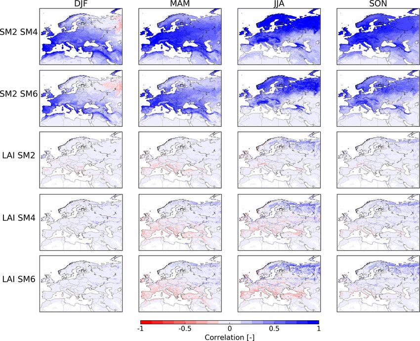
www.hydrol-earth-syst-sci.net/24/325/2020/ Hydrol. Earth Syst. Sci., 24, 325–347, 2020336 B. Bonan et al.: An ensemble square root filter Figure 7. (a) Root mean square difference (RMSD) between observed (rescaled) SSM and its open-loop equivalent for the period 2008–2017 and RMSD difference between assimilation experiments (SEKF in b and EnSRF in c) and the open loop. Figure 8. (a) Correlation (R) between observed (rescaled) SSM and its open-loop equivalent for the period 2008–2017 and R difference between assimilation experiments (SEKF in b and EnSRF in c) and the open loop. ure 9 shows maps of correlations between soil moisture soil. We further notice that SM2 and SM6 are uncorrelated in in layer 2 (1–4 cm depth; SM2, which is used as a proxy summer over Spain and northern Africa. This decorrelation for SSM) and SM in layer 4 (10–20 cm depth; SM4) and between surface and root-zone soil moisture occurs during layer 6 (40–60 cm depth; SM6) and correlations between very dry conditions, such as those which occurred in Spain LAI and SM2, SM4 and SM6. Correlations are averaged by and northern Africa during summer. The same phenomenon season (December–January–February, March–April–May, appears in very arid places such as in the Sahara. SM2 is not June–July–August and September–October–November) over correlated to soil moisture in deeper layers such as SM4 or the whole period 2008–2017. SM6 for each season. This implies that assimilating SSM in The first two rows of Fig. 9 show the seasonal evolution of those areas will not modify soil moisture in deeper layers, as correlations between SM2 and SM4 and SM6. SM4 is highly we will show in the next section. correlated to SM2 (in blue), with R being above 0.5 for most The last three rows of Fig. 9 show the seasonal evolution of places of the domain for each season. SM6 is also highly cor- correlations between LAI and soil moisture in layers 2, 4 and related to SM2, but it is to a lesser extent, meaning that corre- 6. Soil moisture tends to be less correlated on average to LAI lations with SSM decrease in absolute value when we reach than to SSM; nevertheless the values reached are relatively deeper soil layers. We also notice seasonal tendencies. For large (between −0.5 and 0.5). It means that assimilating LAI example, correlations with SM2 tend to be larger in western has an impact on estimated soil moisture. In detail, correla- Europe during spring, while they reach their maximum dur- tions between LAI and SM6 are larger in absolute value than ing summer in Scandinavia. Negative correlations with SM2 SM4 and SM2, meaning that LAI is more correlated to root- (between −0.35 and −0.20) tend to appear during winter zone soil moisture than with SSM. We also observe seasonal over Russia. It means that in those areas in winter, there is geographical patterns. Positive correlations tend to appear in less liquid water in the surface when there is more liquid wa- summer in northern Europe, where deciduous and conifer- ter in deeper layers. This is linked to snow and freezing as we ous forests are dominant, meaning more water in the soil only compare liquid soil moisture from the different layers of leads to a greater LAI. On the contrary in spring and sum- Hydrol. Earth Syst. Sci., 24, 325–347, 2020 www.hydrol-earth-syst-sci.net/24/325/2020/
B. Bonan et al.: An ensemble square root filter 337
Figure 9. Correlation between the model variables sampled from ensembles and averaged seasonally (DJF: December–January–February,
MAM: March–April–May, JJA: June–July–August and SON: September–October–November). From top to bottom: correlation between soil
moisture in the second layer (1–4 cm; SM2) and the fourth layer (10–20 cm; SM4), between SM2 and soil moisture in the sixth layer (40–
60 cm; SM6), between LAI and SM2, between LAI and SM4, and between LAI and SM6. Areas is blue exhibit positive correlations; areas
in red exhibit anti-correlations.
mer, negative correlations appear around the Mediterranean 4.4 Impact of assimilation on soil moisture in deeper
basin. This means a higher LAI leads to reduced soil mois- layers
ture due to plant transpiration in part. Barbu et al. (2011) has
already highlighted this kind of behaviour for Jacobians for Figure 10 displays soil moisture for layers 4 and 6 averaged
grassland places in southwest France. over 2008–2017 from the open loop (left) and the averaged
Overall conclusions drawn from correlations are in ac- difference with SEKF estimates (central panels) and EnSRF
cordance with those derived from the analyses of SEKF estimates (right). We observe that the SEKF and the EnSRF
Jacobians drawn in Albergel et al. (2017) over the Euro- overall have averaged SM4 values similar to the open loop.
Mediterranean region and Tall et al. (2019) over Burkina The main difference occurs in northern Africa and in the Ara-
Faso. Nevertheless, we note that correlation can be influ- bian Peninsula, where the soil is estimated wetter than in
enced by the way we apply model error. Another type of SEKF, with a difference reaching 0.02 m3 m−3 . This dispar-
model error, perturbing for example atmospheric forcing, ity over arid regions in due solely to a wet bias introduced by
may have led to different characteristics of the covariances model error. In those places, EnSRF cannot correct this bias
between the ISBA variables. using observations of SSM or LAI. In other places, EnSRF
can correct the bias potentially introduced by the model per-
turbations to unobserved control variables through the help
of correlations. We also identify greater EnSRF SM4 esti-
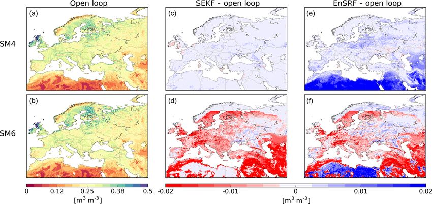
www.hydrol-earth-syst-sci.net/24/325/2020/ Hydrol. Earth Syst. Sci., 24, 325–347, 2020338 B. Bonan et al.: An ensemble square root filter
mates over places such as Poland and Spain, but the differ- EnSRF provides estimates that are more correlated with this
ence with the open loop is always below 0.01 m3 m−3 . independent dataset for almost all grid cells; it improves cor-
Regarding SM6 estimates, both SEKF and EnSRF pro- relation (between 0.05 and 0.1) especially over Spain, north-
duce a drier soil layer than the model for most of the do- ern Africa or around the Caspian Sea, where correlations be-
main as shown in Fig. 10. We identify these patterns for ev- tween the open loop and GLEAM were poorer than for the
ery month without any seasonality (not shown). Also, En- rest of the domain, showing its positive impact on ET. Simi-
SRF SM6 is wetter for regions where bare soil dominates in lar conclusions can be drawn from geographical patterns ob-
northern Africa than SM6 obtained with SEKF or the open served for RMSD and nRMSD (not shown; see Table 1 for
loop. Again this is due solely to the wet bias introduced by averaged results).
model soil moisture perturbations as SM6 and SM2 are un- Figure 13 depicts the correlation between GPP from the
correlated in those places. Then, we can observe for SM6 an FLUXCOM dataset and open-loop estimates (a) and the dif-
abrupt change in the Arctic region for both SEKF and En- ference between correlations for the open loop and the esti-
SRF compared to the open loop. This difference is due to mates produced with SEKF (b) and EnSRF (c). As for ET,
modified hydraulic and thermal soil properties in ISBA for EnSRF provides GPP estimates that are more correlated to
Arctic regions. This modification has been implemented by the FLUXCOM dataset than open-loop and SEKF estimates
Decharme et al. (2016) in order to include a dependency on for almost everywhere, on average 0.817 compared to 0.784
soil organic carbon content. for the model and 0.786 for SEKF. The biggest improve-
Figure 11 shows analysis increments in SM4 for SEKF ments are noticeable around the Caspian Sea (above 0.05),
(top row) and EnSRF (bottom row) for May, July and where correlations between the model and FLUXCOM GPP
September. We see that increments in SM4 tend to be neg- were poorer than for the rest of the domain. Also contrary
ative in May and September in most parts of the domain and to the SEKF, degradations are confined to only few places in
positive in July, particularly in northern Europe for SEKF. Iraq, Iran and close to the Arctic Circle. Again similar con-
The SM4 analyses increments for SEKF and EnSRF tend to clusions can be drawn from geographical patterns observed
be similar, except for arid regions. This makes the SM4 esti- for RMSD and nRMSD (not shown; see Table 1 for averaged
mates less dependent on the data assimilation method. results).
For analysis increments for SM6, SEKF increments are Overall the EnSRF exhibits moderate improvements for
close to zero for every season (not shown). This implies that GPP and ET compared to SEKF.
the drier estimates are solely due to the joint effect of the
ISBA LSM and the updated LAI and soil moisture near the 4.6 Evaluation using river discharges
surface. For EnSRF, this joint effect also occurs, but analysis
increments are not negligible (−0.01 m3 m−3 for the biggest We limit our evaluation to 92 stations over Europe with a
values). The EnSRF SM6 analysis increments compensate model NSE above −1. The NIC of EnSRF compared to the
for the wet bias from model error (not shown) and lead to open loop is displayed for those stations in Fig. 14. Most sta-
similar SM6 estimates as the SEKF in most places as shown tions are located in France and Germany. Blue circles denote
previously. a positive impact (above 3 %) of EnSRF on estimated river
Overall SEKF and EnSRF provide similar estimates for discharges; red circles denote a negative one (below −3 %);
soil moisture in deeper layers for most places but not neces- and grey diamonds denote a neutral impact (between −3 %
sarily through the same mechanisms. and 3 %). A positive NIC is observed for 61 stations and a
negative NIC for only 11 stations. The rest of the stations
4.5 Evaluation using evapotranspiration and gross (20) showed a neutral impact. The largest NIC values are
primary production seen for German stations. Such a positive influence for En-
SRF contrasts with the rather neutral effect of SEKF on river
We now evaluate the performance of our data assimilation discharges. In compliance with previous studies (Albergel et
systems using independent satellite-based datasets of ET and al., 2017; Fairbairn et al., 2017), we observe a significantly
GPP. positive NIC of SEKF for only 15 stations and a negative
The open loop tends to underestimate ET leading to NIC for 3 stations (not shown).
an averaged negative bias of −0.328 kg m−2 d−1 reaching The rather systematic improvement of EnSRF estimates
−0.8 kg m−2 d−1 in June and July. Both SEKF and EnSRF compared to the open loop may be due in part to the assim-
reduce this bias to −0.114 and −0.059 kg m−2 d−1 , respec- ilation of SSM and LAI. It may also be due in part to a bias
tively. More statistics on ET can be found in Table 1. Fig- added by the EnSRF ensemble formulation (as observed for
ure 12 displays correlations between the GLEAM dataset other LSVs) that compensates for an existing bias due to the
and open-loop estimates (a) and the difference between cor- coupling between ISBA and CTRIP. Further investigations
relations for the open loop and the estimates produced with have to be conducted to explore this question. Moreover, a
SEKF (b) and EnSRF (c). Overall the correlation is increased negative NIC is observed for most of the Spanish stations,
on average from 0.789 to 0.803 (SEKF) and 0.823 (EnSRF). where anthropogenic effects (irrigation, importance of dams,
Hydrol. Earth Syst. Sci., 24, 325–347, 2020 www.hydrol-earth-syst-sci.net/24/325/2020/You can also read


