Consistency of satellite-based precipitation products in space and over time compared with gauge observations and snow-hydrological modelling in ...
←
→
Page content transcription
If your browser does not render page correctly, please read the page content below
Hydrol. Earth Syst. Sci., 23, 595–619, 2019
https://doi.org/10.5194/hess-23-595-2019
© Author(s) 2019. This work is distributed under
the Creative Commons Attribution 4.0 License.

Consistency of satellite-based precipitation products in space and
over time compared with gauge observations and snow-
hydrological modelling in the Lake Titicaca region
Frédéric Satgé1,2 , Denis Ruelland3 , Marie-Paule Bonnet2 , Jorge Molina4 , and Ramiro Pillco4
1 CNES,  UMR Hydrosciences, University of Montpellier, Place E. Bataillon, 34395 Montpellier CEDEX 5, France
2 IRD, UMR 228 Espace-Dev, Maison de la télédétection, 500 rue JF Breton, 34093 Montpellier CEDEX 5, France
3 CNRS, UMR Hydrosciences, University of Montpellier, Place E. Bataillon, 34395 Montpellier CEDEX 5, France
4 Universidad Mayor de San Andres, Instituto de Hidraulica e Hidrologia, calle 30 Cota Cota, La Paz, Bolivia

Correspondence: Frédéric Satgé (frederic.satge@ird.fr) and Denis Ruelland (denis.ruelland@um2.fr)

Received: 5 June 2018 – Discussion started: 13 September 2018
Revised: 11 January 2019 – Accepted: 14 January 2019 – Published: 1 February 2019

Abstract. This paper proposes a protocol to assess the space–      precipitation data rather than precipitation derived from the
time consistency of 12 satellite-based precipitation products      available precipitation gauge networks, whereas the SPP’s
(SPPs) according to various indicators, including (i) direct       ability to reproduce the duration of MODIS-based snow
comparison of SPPs with 72 precipitation gauges; (ii) sensi-       cover resulted in poorer simulations than simulation using
tivity of streamflow modelling to SPPs at the outlet of four       available precipitation gauges. Interestingly, the potential of
basins; and (iii) the sensitivity of distributed snow models to    the SPPs varied significantly when they were used to repro-
SPPs using a MODIS snow product as reference in an un-             duce gauge precipitation estimates, streamflow observations
monitored mountainous area. The protocol was applied suc-          or snow cover duration and depending on the time window
cessively to four different time windows (2000–2004, 2004–         considered. SPPs thus produce space–time errors that can-
2008, 2008–2012 and 2000–2012) to account for the space–           not be assessed when a single indicator and/or time window
time variability of the SPPs and to a large dataset com-           is used, underlining the importance of carefully considering
posed of 12 SPPs (CMORPH–RAW v.1, CMORPH–CRT                       their space–time consistency before using them for hydro-
v.1, CMORPH–BLD v.1, CHIRP v.2, CHIRPS v.2, GSMaP                  climatic studies. Among all the SPPs assessed, MSWEP v.2.1
v.6, MSWEP v.2.1, PERSIANN, PERSIANN–CDR, TMPA–                    showed the highest space–time accuracy and consistency in
RT v.7, TMPA–Adj v.7 and SM2Rain–CCI v.2), an unprece-             reproducing gauge precipitation estimates, streamflow and
dented comparison. The aim of using different space scales         snow cover duration.
and timescales and indicators was to evaluate whether the
efficiency of SPPs varies with the method of assessment,
time window and location. Results revealed very high dis-          1     Introduction
crepancies between SPPs. Compared to precipitation gauge
observations, some SPPs (CMORPH–RAW v.1, CMORPH–                   1.1    On the need for and difficulty involved in
CRT v.1, GSMaP v.6, PERSIANN, and TMPA–RT v.7) are                        estimating precipitation fields
unable to estimate regional precipitation, whereas the oth-
ers (CHIRP v.2, CHIRPS v.2, CMORPH–BLD v.1, MSWEP                  Water resources are facing unprecedented pressure due to the
v.2.1, PERSIANN–CDR, and TMPA–Adj v.7) produce a re-               combined effects of population growth and climate change.
alistic representation despite recurrent spatial limitation over   In the 20th century, water extraction underwent a 6-fold in-
regions with contrasted emissivity, temperature and orogra-        crease to sustain food needs and economic levels due to the
phy. In 9 out of 10 of the cases studied, streamflow was           increasing world population (vision, water council, 2000). At
more realistically simulated when SPPs were used as forcing        the same time, global warming has led to the redistribution

Published by Copernicus Publications on behalf of the European Geosciences Union.
596                             F. Satgé et al.: Consistency of satellite-based precipitation products in space and over time

of precipitation, which has favoured the occurrence of both        Japan Aerospace Exploration Agency (JAXA). Over the last
drought and extreme flood events (Trenberth, 2011).                18 years, the TRMM Multisatellite Precipitation Analysis
   As a key component of the hydrologic cycle, it is there-        (TMPA) (Huffman and Bolvin, 2018), the Climate predic-
fore crucial to have accurate precipitation estimates in many      tion centre MORPHing (CMORPH) (Joyce et al., 2004), the
research fields, including hydrological and snow modelling         Precipitation Estimation from remotely Sensed Information
(e.g. Hublart et al., 2016), climate studies (e.g. Espinoza Vil-   using Artificial Neural Networks (PERSIANN) (Sorooshian
lar et al., 2009), extreme flooding (e.g. Ovando et al., 2016),    et al., 2000) and the Global Satellite Mapping Precipitation
drought (e.g. Satgé et al., 2017a), and monitoring to under-       (GSMaP) (GSMaP, 2012) SPP datasets have been developed
stand past and ongoing changes and to optimize water re-           based on the TRMM mission to deliver precipitation esti-
sources management (e.g. Fabre et al., 2015, 2016).                mates at the 0.25◦ grid scale. In 2014, the Global Precipi-
   Measurements of precipitation are usually retrieved from        tation Measurement (GPM) mission was launched to ensure
point gauge stations. Considered as ground truth at the point      TRMM continuity. The second generation of SPPs based on
level, precipitation estimates are then spatialized to represent   GPM missions included the Integrated Multi-SatellitE Re-
the distribution of precipitation in space and over time to be     trievals for GPM (IMERG) (Huffman et al., 2017) and a
used as inputs for impact modelling. However, in most cases,       new GSMaP version product which deliver precipitation es-
the gauge network is too sparse and unevenly distributed to        timates at a finer grid scale (0.1◦ ) than the first generation of
correctly capture the spatial variability of precipitation. This   SPPs but estimates are limited to the period from 2014 to the
is especially true for remote regions such as tropical forests,    present. At the same time, some SPPs took advantage of pre-
mountainous areas and deserts where the usual insufficient         vious SPPs and missions to estimate precipitation over larger
installation and maintenance operations seriously compro-          time window: long-term SPP generation. This is the case
mise precipitation monitoring. An alternative approach con-        of PERSIANN-Climate Data Record (PERSIANN–CDR)
sists in using precipitation derived from weather radar using      (Ashouri et al., 2015), Multi-Source Weighted-Ensemble
the backscattering of electromagnetic waves via hydromete-         Precipitation (MSWEP) (Beck et al., 2017) and Climate Haz-
ors (e.g. Mahmoud et al., 2018). Unlike measurements using         ards Group InfraRed Precipitation (CHIRP) with Station data
traditional gauges, this technique monitors large areas in a       (CHIRPS) (Funk et al., 2015).
distributed way, thus offering the opportunity to monitor pre-        However, SPPs are indirect measurements made from
cipitation over remote regions. However, ground radar mea-         satellite/sensor constellations, including passive microwaves
surements are rarely available at the global or even regional      (PMWs) and infra-red (IR) sensors on board low earth or-
scale (Tang et al., 2016) and are limited in the case of com-      bital (LEO) and geosynchronous satellites, and are subject to
plex terrain which interferes with the radar signal (Zeng et       uncertainty due to technical limitations. Indeed, the irregular
al., 2018). More recently, some authors (Messer et al., 2006;      sampling and limited overpass of LEO PMW measurements
Overeem et al., 2011; Zinevich et al., 2008) reported on           impede the correct capture of short-term and slight precip-
the possibility of estimating precipitation from wireless net-     itation events (Gebregiorgis and Hossain, 2013; Tian et al.,
works such as commercial cellular phone microwave links.           2009) which can introduce error into precipitation estimates
These estimations are based on the attenuation of the electro-     over arid regions and/or during the dry seasons (Prakash et
magnetic signals between telecommunication antennas dur-           al., 2014; Satgé et al., 2016, 2017a; Shen et al., 2010). In
ing precipitation events, and their first results are promising    mountainous regions, the precipitation/no precipitation cloud
(see e.g. Doumounia et al., 2014). However, this technique         classification based on cloud top IR temperature may fail in
faces the problem of private cellular phone company pol-           the case of precipitation processes resulting from orographic
icy about sharing data and telecommunication antenna are           warm clouds (Dinku et al., 2010; Gebregiorgis and Hossain,
mainly located in urban areas, which limits accurate precipi-      2013; Hirpa et al., 2010). The contrast between temperature
tation estimates in space. On the other hand, several satellite-   and emissivity (i.e. water and snow-covered area) of rough
based precipitation estimates (SPPs) are now available, mak-       land surfaces creates background signals similar to those pro-
ing possible to monitor precipitation on regular grids at the      duced by precipitation, leading to misinterpretation between
near global scale, representing an unprecedented opportunity       rainy or not rainy clouds, which can introduce high bias into
to complement traditional precipitation measurements.              precipitation estimates (Satgé et al., 2016, 2018; Tian and
                                                                   Peters-Lidard, 2007; Ferraro et al. 1998; Hussain et al. 2017).
1.2   Satellite-based precipitation estimates (SPPs):                 In addition to these spatial inconsistencies, the orbital
      opportunities and limitations                                satellite context implies constantly varying input data for
                                                                   each observation time (snapshot), which likely introduces
Several SPPs have become available in recent decades to            inhomogeneity into the SPP time records. This could be
monitor precipitation at global scale and on regular grids.        exacerbated by aging sensors and permanent sensor fail-
The first generation of SPPs appeared with the Tropical Rain-      ures. As an example, the TRMM satellite mission ended on
fall Measuring Mission (TRMM) launched in 1997 by NASA             8 April 2015, making unavailable the TRMM Microwave Im-
(National Aeronautics and Space Administration) and the            ager (TMI) from input data used for TMPA retrieval (Huff-

Hydrol. Earth Syst. Sci., 23, 595–619, 2019                                       www.hydrol-earth-syst-sci.net/23/595/2019/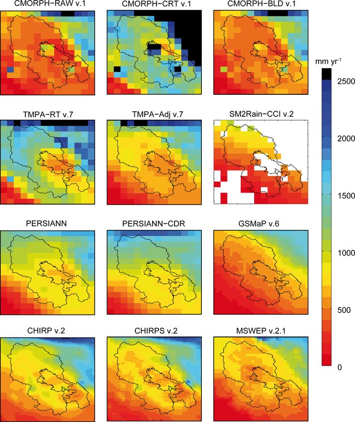
F. Satgé et al.: Consistency of satellite-based precipitation products in space and over time                                  597

man and Bolvin, 2018). Consequently, the potential of SPPs         rank differently depending on the indicator used. For exam-
is expected to present space and time errors whose quantifi-       ple, considering CMORPH, PERSIANN and TMPA datasets
cation is crucial before their use for hydro-climatic studies.     over two African watersheds, TMPA showed the closest esti-
                                                                   mate in comparison with gauges for both basins (Thiemig et
1.3   State-of-the-art evaluation of SPPs                          al., 2012) while CMORPH and TMPA provided more accu-
                                                                   rate streamflow simulations depending on the basin consid-
In the context described above, many studies have reported         ered (Thiemig et al., 2013).
on the efficiency of SPPs over different regions. The most            Whatever the selected approach (based on gauges and/or
common way to evaluate SPP potential is to compare their es-       hydrological modelling), the analysis is performed using a
timates with precipitation gauge measurements, as reviewed         single time window which does not assess the temporal vari-
by Maggioni et al. (2016) and Sun et al. (2018). The compar-       ability of SPPs due to the acquisition process and/or aging
ison of gauge-based assessment studies confirmed the spa-          sensors. To date, only a few studies have been conducted to
tial variability of SPP efficiency in reproducing precipitation,   observe changes in the efficiency of SPPs over time. For ex-
so no single SPP can be said to be the most effective one          ample, CHIRPS precipitation estimates were analysed over
at global scale. For example, when TMPA, CMORPH, and               two distinct time windows to assess potential changes in pre-
PERSIANN SPP datasets were compared, TMPA was found                cipitation accuracy over Cyprus and Nepal from one period
to be closer to the observed precipitation in India (Prakash et    to another (Katsanos et al., 2016; Shrestha et al., 2017). Sim-
al., 2014), the Guyana shield (Ringard et al., 2015), Africa       ilarly, Bai et al. (2018) analysed the accuracy of CHIRPS in
(Serrat-Capdevila et al., 2016), Chile (Zambrano-Bigiarini         mainland China separately for each year to assess its inter-
et al., 2017) and South America Andean plateau (Satgé et           annual variability. These studies highlighted temporal incon-
al., 2016), whereas CMORPH was closer to observed pre-             sistencies in CHIRPS estimates inherent to variations in the
cipitation in Bali, Indonesia (Rahmawati and Lubczynski,           input data used for precipitation retrieval. However, only the
2017), Pakistan (Hussain et al., 2017), and China (Su et           CHIRPS SPP was considered, and similar features are to be
al., 2017; Zeng et al., 2018). However, these assessments          expected with other SPPs.
based on comparison with gauge observations did not assess            Today more than 20 SPPs are available from the first
SPP’s potential performance over unmonitored regions. This         (TRMM), second (GPM) and long-term SPP generation
is especially true for high mountainous regions where avail-       (Beck et al., 2017). Nevertheless, previous studies only con-
able gauge networks (generally located in the valley) cannot       sidered SPP subsets. SPP assessment has indeed focussed on
correctly represent the local precipitation induced by topo-       (i) a single SSP or a limited sample of SPPs (e.g. Cao et al.,
graphic effects. As a result, evaluating SPP potential over        2018; Erazo et al., 2018; Shrestha et al., 2017); (ii) transition
high mountainous regions remains challenging (Hussain et           from the previous to a new version of an algorithm for a spec-
al., 2017; Satgé et al., 2017b).                                   ified SPP (TMPA-v6 to TMPA-v7 for example) (e.g. Chen
   An alternative method consists in assessing the sensitiv-       et al., 2013; Melo et al., 2015; Milewski et al., 2015); and
ity of hydrological models to SPPs. The efficiency of SPPs         (iii) the effectiveness of the transition from the first (TRMM)
can be evaluated indirectly via their ability to generate rea-     to the second (GPM) generation of SPPs (e.g. Satgé et al.,
sonable discharge simulations at the outlet of the basin con-      2017a; Sharifi et al., 2016; Wang et al., 2017). All these stud-
cerned. Compared to gauge-based assessment studies, fewer          ies provided useful feedback related to their specific objec-
authors have reported on hydrological sensitivity to SPPs,         tives but did not really help assess the respective performance
as reviewed in Maggioni and Massari (2018). For example,           of SPPs due to the small sample of SPPs considered.
TMPA, CMORPH and PERSIANN datasets were compared                      For these reasons, comprehensive feedback on SPPs, in-
as forcing data for hydrological modelling in Africa (Casse        cluding space–time consistency, different indicators, insights
et al., 2015; Thiemig et al., 2013; Tramblay et al., 2016) and     into unmonitored regions, and a representative SPP sample,
South America (Zubieta et al., 2015). These studies provided       can only be acquired by backcrossing large SPP assessment
complementary information to gauge-based assessments, of-          studies. Even so, as each study is based on different statisti-
fering an operational overview of SPPs for the management          cal indices, spatial and temporal scales and periods, such an
of water resources. However, due to the aggregation pro-           effort is seriously compromised.
cess at basin scale, the potential of SPPs over specific un-
gauged regions remains unclear. Moreover, in these stud-           1.4   Objectives
ies, the SPPs were not compared with gauge observations
(Thiemig et al., 2013) or provided only a brief comparison         From the previously established state of the art, this paper in-
at basin (Casse et al., 2015; Tramblay et al., 2016) or gauge      vestigates the influence of selected indicators and time win-
(Zubieta et al., 2015) scale. Therefore it is difficult to con-    dows on assessments of the space–time consistency of SPPs.
clude on the respective advantages and limitations of using        The comprehensive protocol relies on different indicators:
gauges or streamflow data as indicators to assess the abil-        (i) gauge observations; (ii) observations of streamflow using
ity of SPPs to reproduce precipitation patterns as SPPs could      sensitivity analysis of a lumped hydrological model in differ-

www.hydrol-earth-syst-sci.net/23/595/2019/                                         Hydrol. Earth Syst. Sci., 23, 595–619, 2019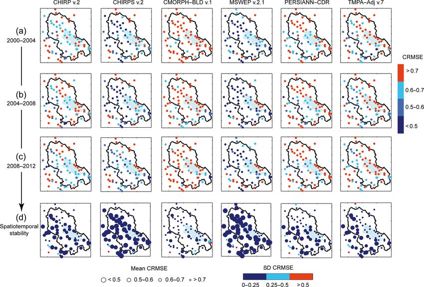
598                             F. Satgé et al.: Consistency of satellite-based precipitation products in space and over time

ent catchments; and (iii) snow cover observed from satellite       2012 period were selected, giving a total of 72 stations in
imagery via sensitivity analysis of a distributed snow model       Bolivia and 51 in Peru (Fig. 1).
in an unmonitored mountainous area, applied to four time              Water level and discharge data from SENAMHI were man-
windows. The aim of using different indicators was to evalu-       aged with the HYDRACCESS free software (Vauchel, 2005)
ate whether the efficiency of the SPPs varies with the assess-     developed by SO-HYBAM to obtain daily discharge records
ment method, whereas different time windows are used to            at the outlet of four catchments (Fig. 1): the Ilave (7766 km2 ),
evaluate a potential variation in SPP performance over time.       the Katari (2588 km2 ), the Keka (801 km2 ), and the Ramis
The Lake Titicaca region was selected as the study area be-        (14 560 km2 ) catchments with respective mean annual dis-
cause it includes all the specific features considered as poten-   charges estimated at 37.3, 2.0, 3.8 and 73.0 m3 s−1 (Uría and
tial limiting factors for SPPs (high mountain massifs, large       Molina, 2013). Nearly complete discharge observations over
water bodies and snow-covered areas) to evaluate the poten-        the 2000–2012 period were available for two basins (Katari
tial of SPPs in an extreme context in terms of the sensors’        and Keka), whereas discharge observations were only avail-
limitations with respect to the orographic effect (i.e. moun-      able from 2008 to 2012 for the other two (Ilave and Ramis).
tains) and high temperature–emissivity contrast (i.e. Lake
Titicaca and a snow-covered region). It also offers the op-        2.2.2    Interpolation of meteorological in situ
portunity to provide feedback on the use of SPPs over poorly                observations
monitored regions.
                                                                   To obtain continuous and spatialized meteorological se-
                                                                   ries for the study area, precipitation and temperature gauge
2     Material: study area and data                                data were interpolated using the inverse distance weighted
                                                                   method (IDW) on a 5 km grid at the regional scale (for de-
2.1     Study area                                                 tails on the purpose of hydrological modelling, see Sect. 3.2)
                                                                   and on a 500 m grid at the local scale (for the purpose of snow
The Lake Titicaca basin is located between 14 and 17◦ S and        modelling, see Sect. 3.3). The choice of the IDW technique
71 and 68◦ W in the northern part of the South American            as interpolation method was based on the study of Ruelland
Andean plateau, known as the Altiplano. It extends over an         et al. (2008), which showed low sensitivity of hydrological
area of 49 000 km2 . The Lake Titicaca catchment is bordered       models to rainfall input datasets derived using different in-
to the west and east by the two Cordilleras (Occidental and        terpolation methods (IDW, Thiessen, spline, ordinary krig-
Real) and includes a few snow-covered areas. With a sur-           ing), with IDW yielding the highest hydrological efficiency.
face area of 8560 km2 , a mean depth of 105 m (284 m max)          Temperature values were interpolated by accounting for a
and a water volume estimated at 903 km3 (Delclaux et al.,          constant lapse rate of 6.5 ◦ C km−1 , in a similar way to that
2007), Lake Titicaca is the main water body and source of          described in Ruelland et al. (2014). Because the gauges are
the endorheic Altiplano hydrologic system. Lake Titicaca is        mainly located in the flat land part of the basins, it was not
drained by the Desaguadero River to the south (Fig. 1) which       possible to provide evidence for an effect of elevation on
contributes up to 65 % of water inflows into Lake Poopó            precipitation distribution. Consequently, no orographic effect
(second largest Bolivian lake) (Pillco and Bengtsson, 2010).       was accounted for in the interpolation of the point precipita-
An accurate Lake Titicaca water balance for monitoring pur-        tion observations. Pref and Tref refer to interpolated precipi-
poses is therefore crucial to support efficient water resources    tation and temperature, respectively.
management in the Altiplano. However, the transboundary,
economic and remote context means hydro-meteorological             2.3     Remote sensing data
monitoring is sparse. Thanks to almost global-scale cover-
age, SPPs represent a promising alternative to monitor re-         2.3.1    Satellite precipitation estimates (SPPs)
gional precipitation in space and over time, and offer an un-
precedented opportunity to achieve efficient regional water        Twelve SPPs with a spatial resolution below or equal to
resources management.                                              0.25◦ (∼ 25 km at the Equator) were selected for the 2000–
                                                                   2012 period. Other precipitation datasets with coarser reso-
2.2     Hydro-climatic data                                        lution (>0.25◦ ) are currently available, but we did not use
                                                                   them because (1) the scarce available gauges network will
2.2.1    Hydro-meteorological stations                             not warrant a consistent potential assessment due to the dif-
                                                                   ference between point-gauge and grid-cell-average measure-
Precipitation and air temperature data for Bolivia were pro-       ment (Tang et al., 2018) and because (2) the considered
vided directly by the Servicio Nacional de Hidrologia e Me-        catchments and snow analysis zone area is smaller than such
teorologia (SENAMHI), whereas for Peru, data were col-             coarse-resolution precipitation datasets. However, it is worth
lected from the Peruvian SENAMHI website. Only weather             mentioning that in specific situations, coarse-resolution SPPs
gauges with less than 20 % daily missing data over the 2000–       could perform better than higher-resolution SPPs (Beck et

Hydrol. Earth Syst. Sci., 23, 595–619, 2019                                       www.hydrol-earth-syst-sci.net/23/595/2019/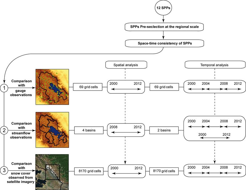
F. Satgé et al.: Consistency of satellite-based precipitation products in space and over time                                         599

Figure 1. Study area: location, meteorological stations (precipitation and temperature observations), streamflow gauges, studied catchments
and snow analysis zone.

al., 2019) and that reanalysis precipitation datasets tend to be        are only delivered at daily scale with a daily aggregation
a better choice in cold regions/periods (Huffman et al., 1995).         based on different time windows which could compromise
Such statements cannot be verified in the present study due to          the comparison of SPPs at daily scale. Finally, using the
the scarce gauge network context and considered catchments              nearest neighbour technique, all the SPPs were spatially re-
and snow analysis zone area.                                            sampled to 5 km to facilitate their comparison. The result-
   The SPPs include the following datasets: Climate Haz-                ing database consists of 10 500 daily virtual stations at 5 km
ards Group InfraRed Precipitation (CHIRP), Climate Pre-                 spatial resolution over the 2000–2012 period for each SPP.
diction Center MORPHing (CMORPH), Global Satellite                      Additionally, SPPs were resampled to 500 m resolution over
Mapping of Precipitation (GSMaP), Precipitation Estima-                 the selected subset region to assess SPP potential for snow
tion from Remotely Sensed Information using Artificial                  modelling (see Fig. 1).
Neural Network (PERSIANN), the Soil Moisture to Rain
(SM2Rain) method, Tropical Rainfall Measuring Mission                   2.3.2   MODIS snow products
(TRMM), Multisatellite Precipitation Analysis (TMPA) and
Multi-Source Weighted-Ensemble Precipitation (MSWEP).                   MOD10A1 (Terra) and MYD10A1 (Aqua) snow products
All the SPPs used a combination of satellite (S) data gather-           version 5 were downloaded from the National Snow and Ice
ing information from passive microwave (PMW) radiome-                   Data Center for the period 24 February 2000–6 January 2016.
ters and infra-red (IR) data from low Earth orbital (LEO)               This corresponds to 5795 daily values among which 5697
and geosynchronous satellites, respectively, except for the             have been available for MOD10A1 (98.3 %) and 4918 for
SM2Rain method, which relies on satellite surface soil mois-            MYD10A1 (84.9 %) since Aqua was launched in May 2002
ture derived from passive and active microwaves. The se-                and became operational in July 2002. These snow products
lected SPPs differ in terms of the combination of satellite             are derived from a NDSI (Normalized Differential Snow
sensors and algorithms and whether the products include re-             Index) calculated from the near-infrared and green wave-
analysis (R) and/or a calibration step against gauge (G) data           lengths, and for which a threshold has been defined for the
in their processing or not. Table 1 provides an overview of             detection of snow. Cloud cover represents a significant limit
these SPPs and relevant references for more information on              for these products, which are generated from instruments op-
their respective production. The mean annual precipitation              erating in the visible–near-infrared wavelengths.
pattern retrieved from all SPPs is presented in Fig. 2.                    As a result, the grid cells were gap-filled so as to pro-
   SPPs were first aggregated to obtain daily time step                 duce daily cloud-free snow cover maps of the study area. The
records using 08:00 to 08:00 local time (LT) time windows               different classes in the original products were first merged
to match local daily gauge observations. It should be noted             into three classes: no-snow (no snow or lake), snow (snow
that some SPPs (CHIRP v.2, CHIRPS v.2 and GSMaP v.6)                    or lake ice), and no-data (clouds, missing data, no decision,
                                                                        and saturated detector). The missing values were then filled

www.hydrol-earth-syst-sci.net/23/595/2019/                                               Hydrol. Earth Syst. Sci., 23, 595–619, 2019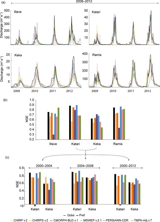
600 F. Satgé et al.: Consistency of satellite-based precipitation products in space and over time
Table 1. Main characteristics and references of the 12 SPPs considered. In the data source column, S stands for satellite, R for reanalysis,
and G for gauge information.
Full name Acronym Data Temporal Temporal Spatial Spatial References
source coverage resolution coverage resolution
Climate Hazard Group CHIRP v.2 S, R 1981–present daily 50◦ 0.05◦ Funk et al. (2015)
InfraRed Precipitation v.2
Climate Hazard Group CHIRPS v.2 S, R, G 1981–present daily 50◦ 0.05◦ Funk et al. (2015)
InfraRed Precipitation with
Station v.2
CPC MORPHing technique CMORPH–RAW v.1 S 1998–present 3h 60◦ 0.25◦ Joyce et al. (2004)
RAW v.1
CPC MORPHing technique CMORPH–CRT v.1 S, G 1998–present 3h 60◦ 0.25◦ Joyce et al. (2004)
bias corrected v.1
CPC MORPHing technique CMORPH–BLD v.1 S, G 1998–present 3h 60◦ 0.25◦ Xie et al. (2011)
blended v.1
Global Satellite Mapping of GSMaP v.6 S, G March 2000– daily 60◦ 0.1◦ Ushio et al. (2009)
Precipitation Reanalyse present Yamamoto et al. (2014)
Gauges v.6
Multi-Source Weighted- MSWEP v.2.1 S, R, G 1979–present 3h Global 0.1◦ Beck et al. (2017)
Ensemble Precipitation v.2.1
Precipitation Estimation from PERSIANN S, G 2000–present 6h 60◦ 0.25◦ Hsu et al. (1997)
Remotely Sensed Information Sorooshian et al. (2000)
using Artificial Neural Networks
PERSIANN-Climate Data PERSIANN–CDR S 1983–2016 6h 60◦ 0.25◦ Ashouri et al. (2015)
Record
TRMM Multi-Satellite TMPA–RT v.7 S 2000–present 3h 60◦ 0.25◦ Huffman et al. (2010)
Precipitation Analysis Real Huffman and Bolvin (2018)
Time v.7
TRMM Multi-Satellite TMPA–Adj v.7 S, G 1998–present 3h 50◦ 0.25◦ Huffman et al. (2010)
Precipitation Analysis Huffman and Bolvin (2018)
Adjusted v.7
Soil Moisture to Rain from SM-Rain–CCI v.2 S 1998–2015 daily Global 0.25◦ Ciabatta et al. (2018)
ESA Climate Change
Initiative v.2
according to a gap-filling algorithm described in Ruelland efficient SPP. However, to avoid overloading the research,
et al. (submitted). This algorithm works in three sequential a pre-selection was made at the Titicaca Lake catchment
steps: (i) Aqua–Terra combination; (ii) temporal deduction scale (hereafter denoted regional scale) to discard less suit-
by sliding the time filter up to 6 days; and (iii) spatial deduc- able SPPs. The remaining SPPs were then assessed using
tion by elevation and neighbourhood filter to gap-fill the re- three successive and complementary methods. The first as-
maining no-data grid cells. The resulting database consists of sessment step consisted of comparing SPPs and gauge obser-
8170 binary (snow/no-snow) daily stations at 500 m spatial vations at the locations of the 69 grid cells which included
resolution for the period 2000–2012 (hereafter Msc ). Finally, gauges. The second assessment step consisted of analysing
snow-covered distribution (SCD) represents the percentage the sensitivity of streamflow modelling to the SPPs at the four
of days with snow and can be retrieved for any grid cells and basin outlets using observed streamflow as reference data.
periods. The third step consisted of analysing the sensitivity of snow
modelling to the SPPs (precipitation datasets) over a subset
mountainous area in the Andes (see Fig. 1) using SCD as ob-
3 A protocol to evaluate the space–time consistency of served from MODIS gap-filled snow products as reference.
satellite precipitation estimates Each assessment step was analysed according to three 4-year
time windows (2000–2004, 2004–2008, 2008–2012) and one
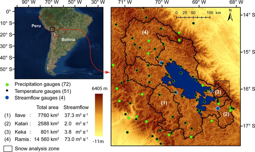
Figure 3 is a flowchart of the main methodological steps. 12-year time window (2000–2012) in which a hydrological
Twelve SPPs were first considered as a representative sam- year corresponds to a period from 1 October to the follow-
ple of currently available SPPs. This is an important con- ing 30 September. The aim of the proposed protocol was
sideration to guide potential SPP users towards the most to investigate the influence of the selected indicator (gauges,
Hydrol. Earth Syst. Sci., 23, 595–619, 2019 www.hydrol-earth-syst-sci.net/23/595/2019/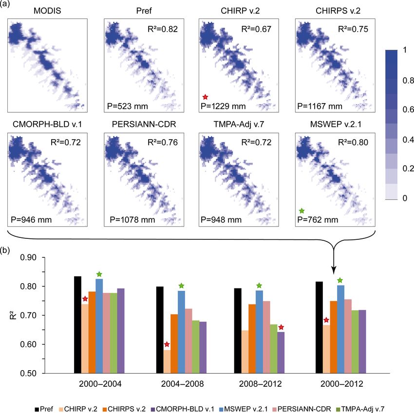
F. Satgé et al.: Consistency of satellite-based precipitation products in space and over time                                            601

                                                                          including at least one precipitation gauge, the daily precipi-
                                                                          tation series from the gauges and SPPs were first aggregated
                                                                          to the 10-day time step over the 12-year period (2000–2012).
                                                                          For each of the 69 0.05◦ grid cells, the 10-day records were
                                                                          only computed when more than 80 % of the daily values
                                                                          were available from all the precipitation datasets (Pref and
                                                                          SPPs) for exactly the same date. Next, mean spatially av-
                                                                          eraged 10-day precipitation series were computed from Pref
                                                                          and all SPPs by aggregating the values from all 69 grid cells.
                                                                          It should be noted that SM2Rain–CCI v.2 estimates rely on
                                                                          soil-moisture observations, with many missing data over wa-
                                                                          ter bodies and mountainous regions (Dorigo et al., 2015),
                                                                          leading to significant spatial gaps over Lake Titicaca and the
                                                                          Cordillera region (Fig. 3). As a result, in comparison to other
                                                                          SPPs, only 44 Pref 0.05◦ grid cells (including gauges) were
                                                                          available for SM2Rain–CCI v.2. Therefore, SM2Rain–CCI
                                                                          v.2 was analysed separately from other SPPs by computing
                                                                          additional Pref and SM2Rain–CCI v.2 mean spatially aver-
                                                                          aged 10-day precipitation series based on the 44 available
                                                                          Pref 0.05◦ grid cells.
                                                                             Mean spatially averaged 10-day SPPs and Pref series for
                                                                          the 12-year period 2000–2012 were compared according to
                                                                          different statistical criteria, namely correlation coefficient
                                                                          (CC), standard deviation (SD), percentage bias (%B) and the
                                                                          centred root mean square error (CRMSE) (Eqs. 1–4):
Figure 2. Mean annual precipitation maps for the 2000–2012 pe-
riod retrieved from all SPPs at their original grid size. For each SPP,          Cov (SPP, Pref )
                                                                          CC =                    ,                                       (1)
only the grid cells with more than 80 % available daily data were                SDSPP × SDref
retained. In order to keep the regional precipitation pattern visible,
black colour was used to filter grid cells whose mean annual precip-      where CC is the correlation coefficient, SPP and Pref are the
itation was greater than 2500 mm yr−1 .                                   SPP and Pref precipitation time series, and Cov is the covari-
                                                                          ance.
                                                                                r
streamflow modelling, snow modelling) and time window to                          1 Xn             2
                                                                          SD =         i=1
                                                                                            Pi − P ,                                (2)
assess the SPPs’ space–time consistency. More details of the                      n
proposed protocol are presented in the following sections. It             where SD is the standard deviation in millimetres, n is the
is noteworthy that the use of a 10-day timescale rather than a            number of values, and P is the precipitation value in mil-
daily timescale may conceal some of the differences among                 limetres (SPP or Pref ).
the datasets, notably by eliminating any insights into their
                                                                                  1 Pn

capacity to capture individual events and higher intensities.                     n  i=1 SPPi − Prefi
However, our choice was based on the inconsistencies we                   %B =         1 Pn
                                                                                                        × 100,                    (3)
                                                                                       n  i=1 Prefi
expected between gauges and daily measurements of SPPs
as a reason to (i) use a different daily time window aggrega-             where %B is the SPP bias value as a percentage, n is the
tion than the local one (08:00 to 20:00) for SPPs delivered at            number of values, SPP is the precipitation estimate of the
daily scale, (ii) the spatial inconsistency between point-gauge           considered SPP value in millimetres, and Pref is the reference
measurement and average grid-cell measurement (Tang et al.,               precipitation value in millimetres.
2018), and (iii) the temporal filters used for gap-filling of                         r
MODIS snow products, which led us to consider that these                                 1 Xn                                  2
reference data were more valid at a 10-day scale than at a                CRMSE =             i=1
                                                                                                   SPPi − SPP − Prefi − Pref , (4)
                                                                                         n
daily scale.
                                                                          where CRMSE is the centred root mean square error in mil-
3.1   Comparison of SPPs with gauge observations:                         limetres, n is the number of values, SPP is the precipitation
      pre-selection and evaluation                                        estimate of the considered SPP value in millimetres, and Pref
                                                                          is the reference precipitation value in millimetres.
SPP consistency was first analysed at the regional scale for                 To facilitate interpretation of the statistical results, the Tay-
the 2000–2012 period. For each of the 69 0.05◦ grid cells                 lor diagram (Taylor, 2001) was used to present obtained CC,

www.hydrol-earth-syst-sci.net/23/595/2019/                                                 Hydrol. Earth Syst. Sci., 23, 595–619, 2019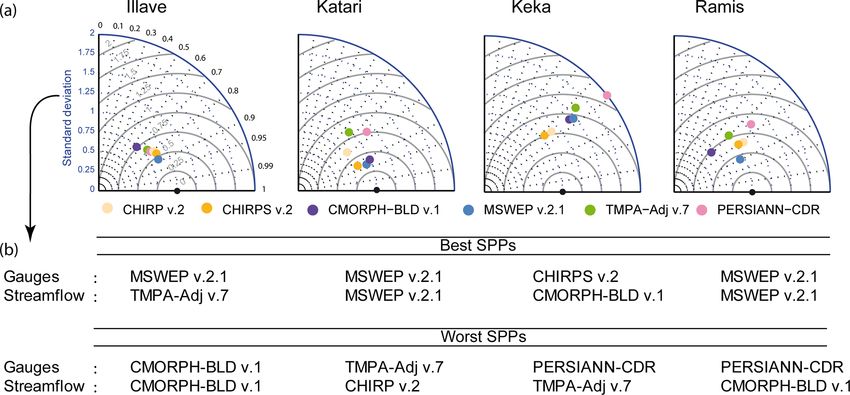
602                               F. Satgé et al.: Consistency of satellite-based precipitation products in space and over time

Figure 3. Flowchart of the main steps from SPP preselection to successive assessment approaches including (1) comparison between SPPs
and gauge observations, (2) sensitivity analysis of runoff modelling to the various SPPs at the four basin outlets and (3) sensitivity analysis
of snow modelling to the various SPPs over a subset mountainous area in the Andes.

and normalized values of SD and CRMSE. Normalization                      periods, respectively. For all the periods considered, 98.6 %
was performed by dividing SPPs CRMSE and SD by Pref                       of Pref grid cells had more than 90 % 10-day records for both
SD. Therefore, in the Taylor diagram, the reference (black                the wet and dry seasons. Consequently, the temporal assess-
dot) corresponds to CRMSE, SD and CC values of 0, 1 and                   ment of the SPPs was not expected to be influenced by any
1, respectively. Also in the Taylor diagram, the position of              inconsistency of Pref over time in terms of available records.
the SPPs relative to the reference dot is an integrated indi-                To assess the spatial consistency of the SPPs, we compared
cator (CRMSE, SD, and CC) of SPP efficiency in reproduc-                  the CC, CRMSE and %B computed between the SPPs and
ing gauge precipitation. The shorter the distance between the             Pref 10-day series for the 2000–2012 period at the location
SPPs and the reference position, the closer the SPPs and Pref             of each grid cell which included gauges. For each SPP, CC,
estimates. Additionally, %B values were used to observe the               CRMSE and %B obtained at the grid-cell level were plot-
potential overestimation/underestimation of each SPP con-                 ted to highlight regions potentially concerned by low (high)
sidered. For the following assessment step, only the six SPPs             SPP potential. We repeated the analysis for the three 4-year
most efficient at the regional scale for 2000–2012 were con-              windows. We only considered CRMSE scores to simplify in-
sidered.                                                                  terpretation of the results, as this score was found to pro-
   To assess the consistency of SPPs over time, mean spa-                 vide more statistical discrimination than CC, SD and %B. It
tially averaged precipitation 10-day series were compared to              is worth mentioning that resampling SPPs (see Sect. 2.3.1)
Pref according to a Taylor diagram for three 4-year periods               could affect the assessment of SPP potential at the grid-cell
corresponding to the 2000–2004, 2004–2008 and 2008–2012                   level. Indeed, at a coarser spatial resolution (0.25◦ ), SPP grid

Hydrol. Earth Syst. Sci., 23, 595–619, 2019                                               www.hydrol-earth-syst-sci.net/23/595/2019/
F. Satgé et al.: Consistency of satellite-based precipitation products in space and over time                                 603

cells’ average precipitation estimates are expected to be more       ity of routing storage (X3, mm), and time base for unit hy-
representative of the mean precipitation derived from all the        drographs (X4, days) for each catchment. Acceptable pa-
gauges in the grid cell considered than the one derived from         rameter bounds were defined according to the recommen-
a single gauge. However, for these particular grid cells, a pre-     dation of Perrin et al. (2003) and previous experiments in
liminary SPP assessment at the original and resampled grid           a similar Andean context (Hublart et al., 2016; Ruelland
sizes revealed no significant differences (data not shown).          et al., 2014). The following ranges were used for model
   Finally, for each grid cell, mean and SD CRMSE values             calibration with all the precipitation datasets tested (Pref
were computed from the three CRMSE values obtained from              and SPPs): 10 mm < X1 < 1800 mm, −5 mm < X2 < 5 mm,
the three 4-year periods. Mean and SD CRMSE values were              1 mm < X3 < 500 mm, 0.5 days < X4 < 5 days. These
then plotted to assess the consistency of SPPs in space and          ranges are large enough to compensate for the differences in
over time. The lower the mean and SD of CRMSE, the more              the different precipitation datasets and basins. Beyond these
stable the SPP considered at the specific grid-cell location.        ranges, we assumed that streamflow simulations could not be
                                                                     realistic. In practice, parameter bounds were rarely reached
3.2    SPPs as input data for hydrological modelling                 when calibrating the model with the different datasets tested
                                                                     (data not shown here for the sake of brevity).
The GR4j lumped hydrological model (Perrin et al., 2003)                The area catchment P - and PE-averaged values were com-
was chosen to analyse the sensitivity of streamflow simula-          puted from the 5 km grid cells P (Pref and SPPs) and PE in-
tions to the various SPPs. The model has demonstrated its            cluded in each catchment considered. We used a weighted
ability to perform well under various hydro-climatic condi-          average based on the 5 km × 5 km fraction included in the
tions (e.g. Coron et al., 2012; Perrin et al., 2003; Grouillet       catchment considered. Pref and SPPs were used sequentially
et al., 2016; Dakhlaoui et al., 2017), notably in the Andean         as forcing precipitation datasets for the streamflow simula-
region (e.g. Hublart et al., 2016).                                  tion. For each run, model parameter calibration was based
   This model relies on daily precipitation (P ) and potential       on the shuffled complex evolution (SCE) algorithm (Duan et
evapotranspiration (PE), which was computed using the for-           al., 1992) by optimizing the Nash–Sutcliffe efficiency crite-
mula proposed by Oudin et al. (2005) (Eq. 5):                        rion (NSE, Eq. 6; Nash and Sutcliffe, 1970) at a 10-day time
                                                                     step. The NSE criterion represents the overall agreement of
       Re T + 5                                                      the shape of the hydrograph, while placing more emphasis
PE =            if (T + 5) > 0; else PE = 0,                  (5)    on high flows. NSE values vary from −∞ to 1, with a max-
       λρ 100
                                                                     imum score of 1 meaning a perfect agreement between the
where PE is daily potential evapotranspiration (mm), Re is           observed and simulated values. By contrast, negative values
extra-terrestrial solar radiation (MJ m−2 d−1 ), which depends       mean that more realistic estimates are obtained using the ob-
on the latitude of the target point and the Julian day of the        served mean values rather than the simulated ones.
year, λ is the net latent heat flux (fixed at 2.45 MJ kg−1 ), ρ is                ( PN
                                                                                              t      t
                                                                                                         2 )
water density (fixed at 11.6 kg m−3 ) and T is the daily mean                          t=1 Qobs − Qsim
                                                                     NSE = 1 − P                         2 ,                  (6)
air temperature (◦ C) estimated at the target point by interpo-                        N
                                                                                            Q t −Q
                                                                                                     sim
                                                                                       t=1    obs
lating the gauge observations while correcting for elevation.
   Firstly, a production module computes the amount of               where NSE is the Nash–Sutcliffe efficiency, Qtobs and Qtsim
water available for runoff, i.e. “effective precipitation”. To       are, respectively, the observed and simulated streamflow for
do so, a soil-moisture accounting (SMA) store is used                time step t, and N is the number of time steps for which
to separate the incoming precipitation into storage, evap-           observations are available.
otranspiration and excess precipitation. At each time step,             The distribution of the basin in the study region (Fig. 1)
soil drainage is computed as a fraction of the storage and           provided the opportunity to assess the hydrological consis-
added to excess precipitation to form the effective precipi-         tency of the SPPs in space by running GR4j in the four basins
tation. Secondly, a routing function split the effective pre-        over the common 2008–2012 period of observed discharge
cipitation into two components: 90 % is routed as delayed            availability. The hydrological consistency of the SPPs over
runoff through a unit hydrograph UH1 in series with a non-           time was then evaluated by running the model over the en-
linear routing storage, while the remaining 10 % is routed           tire 2000–2012 period for which discharge observations were
as direct runoff through a unit hydrograph: UH2 (Perrin et           only available in two catchments (Katari and Keka). For each
al., 2003). UH1 and UH2 consist of slow and quick rout-              precipitation input (Pref and SPPs), the model was calibrated
ing paths, respectively, to account for differences in runoff        against observed streamflow over the whole period (2000–
delays. Finally, the streamflow at the catchment outlet is           2012) and over three 4-year sub-periods (2000–2004, 2004–
computed by summing up delayed and direct runoff. This               2008, and 2008–2012). No validation step was used as the
model relies on four calibrated parameters: maximum capac-           objective was to assess hydrological modelling sensitivity to
ity of the soil moisture accounting store (X1, mm), inter-           various precipitation datasets (Pref and SPPs) and not to as-
catchment exchange coefficient (X2, mm), maximum capac-              sess the hydrological model robustness under climate vari-

www.hydrol-earth-syst-sci.net/23/595/2019/                                          Hydrol. Earth Syst. Sci., 23, 595–619, 2019
604 F. Satgé et al.: Consistency of satellite-based precipitation products in space and over time
ability. The aim of the analysis of the streamflow simulation initial conditions (data not shown). An initial 3-year warm-
accuracy among the basins and periods considered was thus up period was used for each simulation to limit the influence
to evaluate the strength of the SPPs in space and over time of these conditions.
and discrepancies in reproducing streamflow. The following ranges were used for model calibra-
tion with all the tested precipitation datasets (Pref
3.3 SPPs as input data for snow modelling in the Andes and SPPs): 0.5 mm ◦ C−1 d−1 < Kf < 20 mm ◦ C−1 d−1 ,
1 mm < SWEth < 80 mm. Kf ranges were based on ranges
A distributed degree-day model (Ruelland et al., 2019) was adapted from the values reviewed in Hock (2003). Re-
chosen to analyse the sensitivity of snow cover simula- garding the SWEth value, the assumption is that, using
tions to the SPPs. This storage-based model relies on daily remote sensing, snow cover cannot be detected below a
distributed precipitation (P ), temperature (T ) and potential certain threshold (Bergeron et al., 2014). For instance,
evaporation (PE) (Eq. 7) to represent the main snow accu- based on in situ measurements to detect snow cover from
mulation and ablation (sublimation and melt) processes (see MODIS in the Pyrenees, Gascoin et al. (2015) found a mean
Fig. 4). It operates at a daily time step according to a grid threshold of 40 mm. Since this value may be influenced by
of 500 × 500 m corresponding to the spatial resolution of the the local context (vegetation, topography, and climate) and
MODIS data. spatial difference between point (in situ) and areal satellite
Snow accumulation is defined using a temperature thresh- (MODIS) observations, SWEth was tested according to
old Ts fixed at 0 ◦ C. Sublimation is accounted for based on large ranges. It is worth mentioning that the tested bounds
daily PEsub (mm) at the target grid cell and snowmelt is con- were reached during calibration for all simulations (i.e.
trolled with a melt factor parameter Kf (◦ C−1 d−1 to be cali- Kf = 20 mm ◦ C−1 d−1 and SWEth = 1 mm). However, we
brated) according to Eqs. (8)–(9). did not consider larger parameter ranges to ensure “realistic”
simulations.
PEsub = PE × Ksub , (7) In association with Tref for temperature forcing data (see
Sect. 2.2), Pref and SPPs were sequentially used as forcing
where PEsub is potential evapo-sublimation, PE is potential precipitation datasets to simulate snow cover with the model.
evaporation (see Eq. 5), and Ksub is a proportional coefficient For each run, model parameters were calibrated based on the
depending on the mean latitude (lat, decimal degrees) of the shuffled complex evolution (SCE) algorithm by optimizing
study area and varying from 0 at the poles to 1 at the Equator the grid-cell-to-grid-cell correlation between the snow cover
(see Ruelland et al., 2019 for more details): duration (SCD) simulated by the model and that observed by
the gap-filled MODIS snow products (see Sect. 2.3.2), ac-
Mf = Kf × (T − Ts) , (8) cording to the following Eq. (10):
0 Tj ≤ Ts
Melt = , (9) 2
Min (SWE, Mf) Tj > Ts Pn
SCDMODIS(p) − SCDMODEL(p)
2 p=1
R = 1− , (10)
where Mf is the potential melt (mm), Kf is a melt factor pa- Pn 2
p=1 SCDMODIS(p)
rameter to be calibrated, T is the temperature on day j on
the grid cell considered, and Ts is the threshold temperature where R 2 is a determination coefficient, n is the total num-
parameter (fixed at 0 ◦ C) for snow accumulation and melt. ber of grid cells in the study area (see Fig. 1), p is a given
Melt cannot exceed the snow water equivalent (SWE) of the grid cell, and SCDMODIS and SCDMODEL are, respectively,
snowpack storage. the snow cover duration (SCD) observed by MODIS and the
The snow-covered areas (SCAs) are estimated from the SCD simulated by the model as a percentage of days over the
SWE. For each grid cell, snow is stored in a reservoir which analysis period.
represents the SWE of the grid-cell snowpack (see Fig. 4). For each precipitation input (Pref and SPP), the model
It is fed solely by the solid fraction of precipitation and is was calibrated against MODIS observed snow cover over the
emptied according to the simulated sublimation and melt pro- entire period 2000–2012 and over three 4-year sub-periods
cesses. For each model, a grid cell is assigned to snow or not (2000–2004, 2004–2008, and 2008–2012). The aim of the
depending on a water level threshold SWEth (mm), to be cal- analysis of the snow simulation accuracy among the areas
ibrated. and periods considered was to evaluate the strength of SPPs
As the region contains permanent snow-covered areas, for in space and over time and to identify discrepancies in repro-
grid cells located below and above 5700 m a.s.l., the SWE ducing snow cover in a remote Andean area (see Fig. 1).
reservoir was initialized to 0 and 300 mm, respectively, at
the beginning of the simulations. These values were defined
based on MODIS snow observations and on model sensitivity
tests to SWE initial conditions accounting for different ele-
vation thresholds. The analysis revealed limited sensitivity to
Hydrol. Earth Syst. Sci., 23, 595–619, 2019 www.hydrol-earth-syst-sci.net/23/595/2019/F. Satgé et al.: Consistency of satellite-based precipitation products in space and over time 605
CHIRP v.2, CHIRPS v.2, CMORPH–BLD v.1, PERSIANN–
CDR, TMPA–Adj v.7, and MSWEP v.2.1.
At the regional scale, SPP rank performance remained
stable during the time windows considered and similar to
what was observed for the 2000–2012 period (Fig. 5). There-
fore, at the regional scale, SPPs were generally consis-
tent over time, MSWEP v.2.1 being the most accurate and
PERSIANN–CDR the least accurate SPP. However, for the
2008–2012 period, CHIRPS v.2 and CHIRP v.2 were closer
than for the previously considered period. This might be due
to the decrease in the number of available gauges for the ad-
justment processes applied to CHIRP v.2 to produce CHIRPS
v.2.
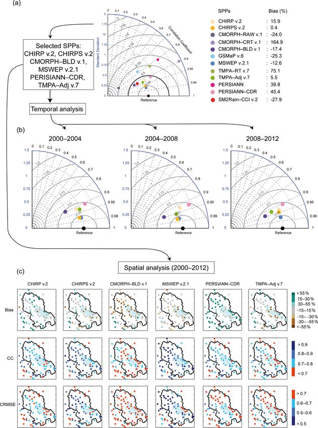
Figure 5c shows the spatial distribution of SPP errors for
the 2000–2012 period in terms of %B, CC, and CRMSE.
CMORPH–BLD v.1 was poorly correlated with Pref , with
the highest proportion of grid cells with CC less than 0.7.
Figure 4. Distributed degree-day model used in the study (Ruelland This value is generally used as a quality threshold with CC
et al., 2019). values less than 0.7 indicating poor SPP performance (see
e.g. Satgé et al., 2016). MSWEP v.2.1 had the best CC value
overall, with the highest proportion of grid cells with a CC
greater than 0.9 and only two grid cells with unsatisfactory
4 Results
CC values.
The main differences were in %B and CRMSE.
4.1 Space–time consistency of SPPs compared with CMORPH–BLD v.1 and PERSIANN–CDR precipitation un-
gauge observations derestimations and overestimations at the regional scale
(Fig. 5a) were confirmed at the gauge scale (Fig. 5c). CHIRP
SPPs are distributed over the Taylor diagram, indicating high v.2, CHIRPS v.2, and TMPA–Adj v.7 presented similar %B
discrepancy among them for the 2000–2012 period (Fig. 5a). distribution, while MSWEP v.2.1 had the most homogeneous
Some SPPs greatly overestimated precipitation, with %B %B distribution, with the values of almost all grid cells rang-
values of 165 %, 75 %, 40 % and 45 % for CMORPH–CRT ing between −30 % and +30 %. This range was previously
v.1, TMPA–RT v.7, PERSIANN and PERSIANN–CDR, re- defined as satisfactory %B for SPPs (Shrestha et al., 2017).
spectively. CMORPH–RAW v.1, GSMaP v.6 and SM2Rain– The gauge adjustment applied to CHIRP v.2 was globally
CCI v.2 greatly underestimated precipitation, with %B val- positive, with a %B reduction from CHIRP v.2 (15.9 %) to
ues of −24 %, −25 % and −37 %, respectively. However, all CHIRPS v.2 (0.4 %) of almost 100 % (Fig. 4a). It consider-
SPPs were highly correlated with Pref with CC greater than ably increased the numbers of grid cells with %B between
0.75. Generally, including gauge data in the SPP processing −15 % and +15 % from CHIRP v.2 to CHIRPS v.2 (Fig. 5b)
clearly enhanced precipitation estimates. Indeed, CHIRPS and generally enhanced CRMSE and CC scores.
v.2, CMORPH–BLD v.1, PERSIANN–CDR and TMPA–Adj Interestingly, all the SPPs underestimated precipitation for
v.7 were closer to the reference dot than their respective non- the two grid cells located over the northern Lake Titicaca is-
adjusted versions, CHIRP v.2, CMORPH–RAW v.1, PER- lands. This is probably linked to SPP’s limited ability to de-
SIANN and TMPA–RT v.7. With the closest and farthest dis- tect warm cloud precipitation (see Sect. 5.1).
tance to the reference, MSWEP v.2.1 and CMORPH–CRT CMORPH–BLD v.1, PERSIANN–CDR, and TMPA–Adj
v.1 were, respectively, the most and least consistent SPPs to v.7 had the highest proportion of grid cells with CRMSE val-
represent the mean spatially averaged precipitation over the ues greater than 0.7 (Fig. 5c). This value can be used as a
2000–2012 period. quality threshold above which SPP performance is consid-
According to the literature, a quality threshold value can ered unsatisfactory (see e.g. Shrestha et al., 2017). Therefore,
be used to express SPP potential. Some authors (e.g. Hussain over the 2000–2012 period, precipitation estimates derived
et al., 2017; Satgé et al., 2016; Shrestha et al., 2017) consid- from CMORPH–BLD v.1, PERSIANN–CDR and TMPA–
ered a normalized RMSE value lower than 0.5 to be associ- Adj v.7 are subject to high uncertainties at local scale. The
ated with a very good SPP performance. Even though there inclusion of gauge observations for CHIRPS v.2 estimates
were slight differences between CRMSE and RMSE, the use reduced the number of grid cells with unsatisfactory perfor-
of a normalized CRMSE threshold value of 0.5 to select only mance by 50 % in comparison with the non-adjusted CHIRP
the most efficient SPPs remains logical. Therefore, six SPPs v.2 version. With only 14 and 12 grid cells with CRMSE
were selected for the following assessment steps, including
www.hydrol-earth-syst-sci.net/23/595/2019/ Hydrol. Earth Syst. Sci., 23, 595–619, 2019606 F. Satgé et al.: Consistency of satellite-based precipitation products in space and over time Figure 5. Efficiency of SPPs compared with gauge observations: (a) pre-selection of SPPs at the regional scale in the form of a Taylor diagram; (b) consistency of SPPs over time at the regional scale in the form of a Taylor diagram; and (c) consistency of SPPs in space for the 2000–2012 period from CC, CRMSE and %B values obtained from each Pref grid cell including at least one gauge. Hydrol. Earth Syst. Sci., 23, 595–619, 2019 www.hydrol-earth-syst-sci.net/23/595/2019/
F. Satgé et al.: Consistency of satellite-based precipitation products in space and over time                                 607

greater than 0.7, respectively, CHIRPS v.2 and MSWEP v.2.1         4.2   Space–time consistency of SPPs compared with
showed the highest spatial consistency.                                  streamflow simulations
   More generally, the spatial analysis highlighted three areas
in which all the SPPs considered presented less satisfactory       Streamflow simulations using Pref varied along the catch-
statistical scores (CRMSE, CC, and %B) than over the re-           ments, with the lowest NSE score of 0.63 for Keka and the
maining areas. These regions correspond to the south-eastern       highest of 0.89 for Katari. Simulated SPP streamflow effi-
Lake Titicaca shore, and the south-western and north-eastern       ciency followed the same trend, except with CMORPH–BLD
borders of the catchment.                                          v.1 and TMPA–Adj v.7 (Fig. 7). TMPA–Adj v.7 provided
   The SPPs’ lowest potential over the south-eastern shore         the best streamflow simulation for the Ilave catchment and
of Lake Titicaca and at the south-western and north-eastern        the worst for Keka, whereas the opposite was observed us-
borders of the catchment highlighted in the 2000–2012 pe-          ing CMORPH–BLD v.1 as forcing data. The low efficiency
riod was confirmed for all four time windows, as indicated by      of CMORPH–BLD v.1 in the Ilave catchment was related
CRMSE values (Fig. 6). For each time window, the CRMSE             to its erroneous streamflow peaks in the 2009 and 2012 dry
distribution differed depending on the SPP considered. More        seasons. CHIRP v.2 and CMORPH–BLD v.1 had the lowest
interestingly, the distribution of CRMSE of all the SPPs dif-      scores for the Katari and Ramis catchments, with NSE values
fered depending on the time window considered. As a re-            of 0.59 and 0.45, respectively. For all the catchments, stream-
sult, the efficiency of the SPPs varied over time for a spe-       flow simulations based on CHIRPS v.2 presented systemati-
cific region (at the grid-cell scale). As a clear example, for     cally higher NSE scores than simulations based on CHIRP
the CMORPH–BLD v.1 south-eastern located grid cells, the           v.2, showing that the adjustment provided in CHIRPS v.2
CRMSE values changed drastically over time: these grid             with the integration of gauge observations led to better pre-
cells presented unsatisfactory CRMSE scores (above 0.7) for        cipitation estimates. This confirms the enhancement of the
the 2000–2004 period and satisfactory CRMSE scores (be-            gauge-based assessment observed with an overall reduction
low 0.5) for both the 2004–2008 and 2008–2012 periods.             in bias and an increase in CRMSE and CC.
   In this context, Fig. 6d represents the space–time consis-         For all the catchments considered, the best streamflow
tency of the SPPs over the 2000–2012 period. The mean and          simulations were obtained with at least one of the SPPs as
SD CRMSE values obtained at the location of each grid cell         forcing precipitation data. TMPA–Adj v.7 and CMORPH–
in the three sub-periods considered, used as indicators of the     BLD v.1 provided a better streamflow simulation than Pref
space–time consistency, are plotted in Fig. 6d. Overall, all       for Ilave and Keka, respectively, and MSWEP v.2.1 outper-
SPPs are stable in space and over time, with SD CRMSE              formed Pref for the Katari and Ramis catchments. These re-
values below 0.25, but their consistency differed in accuracy.     sults show that SPPs can efficiently replace the currently
CMORPH–BLD v.1 provided stable but not accurate precip-            available sparse precipitation gauge networks for use in hy-
itation estimates, with mean CRMSE values systematically           drological studies of the region. Overall, MSWEP v.2.1 ap-
above 0.7. In contrast, MSWEP v.2.1 and CHIRPS v.2 pre-            pears to be the most consistent SPP product for streamflow
sented stable and accurate precipitation estimates, with many      simulations. Indeed, the streamflow simulations forced by
grid cells with a mean CRMSE below 0.5. CHIRP v.2 space–           MSWEP v.2.1 were more realistic than those forced by Pref
time consistency was lower than that of CHIRPS v.2, thereby        over three catchments (Katari, Keka, and Ramis) and were
confirming the advantage of the gauge calibration (Fig. 6d).       almost the same for the Ilave catchment.
PERSIANN–CDR and TMPA–Adj v.7 were more consistent                    However, as shown in Fig. 7c, the SPP hydrological rank-
in space and over time over the southern mid and western re-       ing in the 2008–2012 period changed drastically over time.
gions, respectively. Interestingly, the close potential precipi-   For example, for the Katari catchment, MSWEP v2.1 led
tation estimates observed for CHIRP and CHIRPS v.2 at the          to the best streamflow simulations for the 2004–2008 and
regional scale and for the 2008–2012 period were confirmed         2000–2012 periods but not for the 2000–2004 period, for
at the grid-cell level, with similar spatial error distribution    which TMPA–Adj v.7 forced streamflow simulations had a
for both SPPs. Therefore, gauge adjustment appears to be           higher NSE score of 0.85. Additionally, CMORPH–BLD v.1
less efficient for the 2008–2012 than for the 2000–2004 and        potential fell drastically over the 2000–2004 period with a
2004–2008 periods.                                                 negative NSE score, whereas it produced the most realis-
   MSWEP v.2.1 and CHIRPS v.2 were the most stable SPPs            tic streamflow simulation for the period 2008–2012. In the
in space and over time, with the highest proportion of grid        Keka catchment, for each time window, the best streamflow
cells with a mean and a SD CRMSE below 0.5 and 0.25, re-           simulation was obtained using different SPPs. CHIRP v.2,
spectively (Fig. 6d). However, for grid cells located on the       PERSIANN–CDR and CMORPH–BLD v.1 resulted in the
south-eastern shore of the lake, CHIRPS v.2 provided more          highest NSE scores over the various sub-periods analysed,
accurate and stable precipitation estimates than MSWEP             with, respectively, 0.73 for the period 2000–2004, 0.83 for
v.2.1 and all the other SPPs.                                      2004–2008 and 0.77 for 2008–2012.
                                                                      To conclude, the analysis of streamflow model sensitivity
                                                                   to the different precipitation datasets depended to a great ex-

www.hydrol-earth-syst-sci.net/23/595/2019/                                        Hydrol. Earth Syst. Sci., 23, 595–619, 2019
You can also read