The role and value of distributed precipitation data in hydrological models - HESS
←
→
Page content transcription
If your browser does not render page correctly, please read the page content below
Hydrol. Earth Syst. Sci., 25, 147–167, 2021
https://doi.org/10.5194/hess-25-147-2021
© Author(s) 2021. This work is distributed under
the Creative Commons Attribution 4.0 License.

The role and value of distributed precipitation
data in hydrological models
Ralf Loritz1 , Markus Hrachowitz2 , Malte Neuper1 , and Erwin Zehe1
1 Karlsruhe   Institute of Technology (KIT), Institute of Water and River Basin Management, Karlsruhe, Germany
2 Delft   University of Technology, Faculty of Civil Engineering and Geosciences, Delft, the Netherlands

Correspondence: Ralf Loritz (ralf.loritz@kit.edu)

Received: 30 July 2020 – Discussion started: 3 August 2020
Revised: 18 November 2020 – Accepted: 20 November 2020 – Published: 7 January 2021

Abstract. This study investigates the role and value of dis-     flow at the outlet of a catchment (e.g., Das et al., 2008). Al-
tributed rainfall for the runoff generation of a mesoscale       though the generality of such findings is surely limited by the
catchment (20 km2 ). We compare four hydrological model          fact that distributed models have more parameters that need
setups and show that a distributed model setup driven by dis-    to be identified, which makes model calibration much more
tributed rainfall only improves the model performances dur-      challenging (Beven and Binley, 1992; Huang et al., 2019),
ing certain periods. These periods are dominated by convec-      they highlight the ability of the hydrological system to dis-
tive summer storms that are typically characterized by higher    sipate spatial gradients efficiently (e.g., Obled et al., 1994).
spatiotemporal variabilities compared to stratiform precip-      This is the case as hydrological processes are strongly dis-
itation events that dominate rainfall generation in winter.      sipative but exhibit, despite the nonlinearity of surface and
Motivated by these findings, we develop a spatially adap-        subsurface flow processes, no chaotic behavior (Berkowitz
tive model that is capable of dynamically adjusting its spa-     and Zehe, 2020).
tial structure during model execution. This spatially adap-         In contrast to the above-mentioned finding that hydrologi-
tive model allows the varying relevance of distributed rain-     cal systems can efficiently dissipate spatial gradients, several
fall to be represented within a hydrological model without       other studies showed that information about the spatial vari-
losing predictive performance compared to a fully distributed    ability of precipitation can significantly improve the predic-
model. Our results highlight that spatially adaptive modeling    tive performance of hydrological models. For instance, Euser
has the potential to reduce computational times as well as       et al. (2015) highlighted that distributed models driven by
improve our understanding of the varying role and value of       distributed rainfall could reproduce the observed hydrograph
distributed precipitation data for hydrological models.          of a 1600 km2 large catchment in Belgium with higher ac-
                                                                 curacy compared to spatially lumped model structures. Fur-
                                                                 thermore, Woods and Sivapalan (1999) showed that the in-
                                                                 terplay between spatial patterns of rainfall and soil saturation
1   Introduction                                                 can substantially impact the runoff generation of a catchment
                                                                 when they analyzed the dependence of average runoff rates
“How important are spatial patterns of precipitation for the     on the spatial and temporal variability of the meteorologi-
runoff generation at the catchment scale?” This is a key         cal forcing and the catchment state. The relevance of these
question for the application of hydrological models that         spatial patterns is thereby particularly high if the system is
has been addressed in several studies over the past decades      close to a threshold where different localized preferential
(e.g., Beven and Hornberger, 1982; Smith et al., 2004; Lobli-    flow processes start to dominate (e.g., cracking soils: drying
geois et al., 2014). A frequently drawn conclusion is that       of soil; macropores: occurrence of earthworms) as discussed
semi-distributed or even lumped models driven by a single        by Zehe et al. (2007). Spatial averaging of the system state or
precipitation time series often outperform distributed models    the meteorological forcing can hence lead to a misrepresen-
with respect to their ability to reproduce observed stream-

Published by Copernicus Publications on behalf of the European Geosciences Union.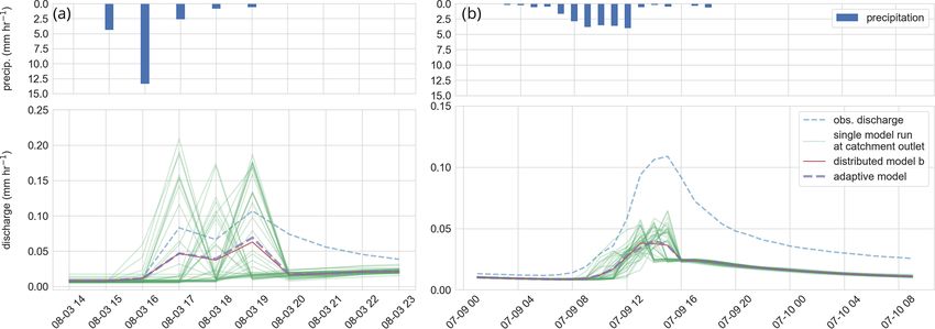
148                            R. Loritz et al.: The role and value of distributed precipitation data in hydrological models

tation of relevant spatial patterns, especially at more extreme     multiple new problems, for instance, how to infer the ini-
conditions.                                                         tial conditions of a catchment prior to a rainfall event given
   Given the partly contradictory findings present in the lit-      the degrees of freedom distributed models can offer (Beven,
erature, it appears reasonable to assume that the relevance         2001). The latter is of considerable importance, particularly
of distributed rainfall is changing dynamically over time and       during extremes resulting from high-intensity rainfall-runoff
depends on the interplay of the prevailing (i) system state         events, which can be strongly sensitive to the actual state of
(e.g., catchment wetness); (ii) the system functional struc-        the system such as the spatial patterns of macropores (Zehe
ture, determined by patterns of topography, land use, and           et al., 2005) or of the antecedent soil water content (Zehe and
geology; and well as (iii) the strength and spatial organiza-       Blöschl, 2004).
tion of the rainfall forcing. In consequence, it seems further-        A different avenue to implement a dynamically changing
more rational to hypothesize that also hydrological models          model resolution is adaptive clustering, as recently demon-
should dynamically adapt their spatial structure to the pre-        strated for a spatially distributed conceptual (top-down)
vailing context, thereby reflecting the inherently dynamic na-      model by Ehret et al. (2020). This concept allows for con-
ture of hydrological similarity (Loritz et al., 2018).              tinuous hydrological simulations, which use a higher spatial
   The idea that hydrological models should dynamically al-         model resolution only at those time steps when it is neces-
locate their spatial resolution, as well as the associated rep-     sary. The idea behind adaptive clustering is similar to adap-
resentation of natural heterogeneity in time, is motivated by       tive time stepping (e.g., Minkoff and Kridler, 2006). How-
our previous work (Loritz et al., 2018). In that study, we high-    ever, instead of reducing the time steps during times when
lighted that simulations of a distributed model consisting of       large gradients prevail, adaptive clustering increases or de-
105 independent hillslopes were highly redundant to repro-          creases the number of independent spatial model elements
duce discharge or catchment storage changes of a mesoscale          during times of low or high functional diversity. The gen-
catchment within 1 hydrological year. Based on the Shannon          eral concept behind adaptive clustering is thereby not entirely
entropy as a metric, we identified periods in which a rather        new to environmental science and is already used for in-
small number of representative hillslopes was sufficient be-        stance in hydrogeology under the term “adaptive mesh”, with
cause most of them functioned largely similarly within the          the main focus to increase the resolution of gradients during
chosen margin of error. However, during other periods, up to        times of high dynamics by increasing or decreasing the num-
32 independent representations of hillslopes were required,         ber of nodes (grid elements) in a model (Berger and Oliger,
which underlines that spatial variability of system proper-         1984). The main difference between the adaptive mesh and
ties, such as surface topography or soil types among the hill-      adaptive clustering approach is that instead of adjusting the
slopes, can exert a stronger influence on the runoff genera-        spatial resolution of the numerical grid during runtime, adap-
tion at certain times, as expected given the findings reported      tive clustering changes the number of hydrological response
by other studies conducted in the same research environment         units (HRUs) that are used (needed) to represent a catchment.
(e.g., Fenicia et al., 2016; Loritz et al., 2017). It can, there-   This implies that also the degree of spatial heterogeneity of
fore, be argued that distributed rainfall and corresponding         the catchment state (e.g., the soil moisture or energy state)
distributed model structures are also only important during         that is covered by the model is dynamically changing.
specific periods, while during other periods a compressed,             While the idea of adaptive clustering is promising as it al-
spatially aggregated model structure may be sufficient. An          lows a minimum adequate representation of the spatial vari-
implementation of such an adaptive spatial model resolu-            ability of a hydrological landscape, it has, to the best of our
tion would ensure an appropriate spatial model complexity,          knowledge, so far only been tested within a simple top-down
defined based on the least number of details about the sys-         model (Ehret et al., 2020). It is thus of interest whether such
tem structure (e.g., the variability of topographic gradients)      a dynamic clustering is also feasible when using a physi-
and catchment states that are sufficient to capture the rele-       cally based (bottom-up) model particularly as these mod-
vant interactions with the spatial pattern of precipitation. Yet    els were specifically introduced to explore how distributed
it would be as parsimonious as possible to avoid redundant          system characteristics and driving gradients control hydro-
computations, which again could be used to minimize com-            logical dynamics (Freeze and Harlan, 1969). Here we will
putational costs (Clark et al., 2017).                              hence test and develop an adaptive clustering approach us-
   Moving to the event timescale instead of running continu-        ing straightforward physical reasoning and implement it into
ous simulations is surely one way to achieve such a dynam-          a distributed bottom-up model. The overarching objective
ical allocation of the model space and means to use differ-         of this study is thus to exploit the value of adaptive clus-
ent model setups with different spatiotemporal resolutions          tering as a tool to better understand the temporal relevance
at different times. This would entail running a set of mod-         of distributed precipitation for the runoff generation of a
els that differ with respect to their resolutions in space and      mesoscale catchment and, as a by-product, to reiterate that
time, depending on the prevailing structure of the meteoro-         adaptive clustering could potentially be used to reduce com-
logical forcing and current state of a hydrological landscape       putational times, as already discussed in detail by Ehret et
(e.g., the soil moisture or energy state). Yet, this introduces     al. (2020). High computational times are thereby still one of

Hydrol. Earth Syst. Sci., 25, 147–167, 2021                                           https://doi.org/10.5194/hess-25-147-2021
R. Loritz et al.: The role and value of distributed precipitation data in hydrological models 149
the many reasons why bottom-up models are rarely used on
larger scales in an spatial explicit manner (Clark et al., 2017).
For instance, Hopp and McDonnell (2009) used the HY-
DRUS 3D model (e.g., latest version of HYDRUS; Šimunek
et al., 2016) and reported computational times ranging from
10 min up to 11 h when they simulated water fluxes and
state variables at the Panola hillslope (area = 0.001250 km2
(25 m × 50 m); maximal soil depths = 4 m) for a simulation
time of 15 d by changing slope angles, soil depths, storm
sizes, and bedrock permeability. A meaningful application
of bottom-up models at relevant management scales (around
250 km2 in south Germany; e.g., Loritz, 2019), without a vi-
olation of important physical constraints (e.g., 10−2 –101 m
maximum vertical grid size for the Richards equation; Or et
al., 2015; Vogel and Ippisch, 2008), would thus imply long
computational times. This again strongly limits the number
of feasible model runs to examine, for instance, different pa-
rameter sets (Beven and Freer, 2001).
In this study, we therefore test the specific hypothesis
that adaptive clustering is a feasible approach to represent
the spatial variability of rainfall in a hydrological bottom-
up model at the lowest sufficient level of detail without los-
ing predictive performance compared to a fully distributed
model. We test this hypothesis by introducing a clustering
approach for the example of the model CATFLOW applied to
the 19.4 km2 Colpach catchment using a gridded radar-based
quantitative rainfall estimate by addressing the two following
research questions:
1. Does the model performance of a spatially aggregated
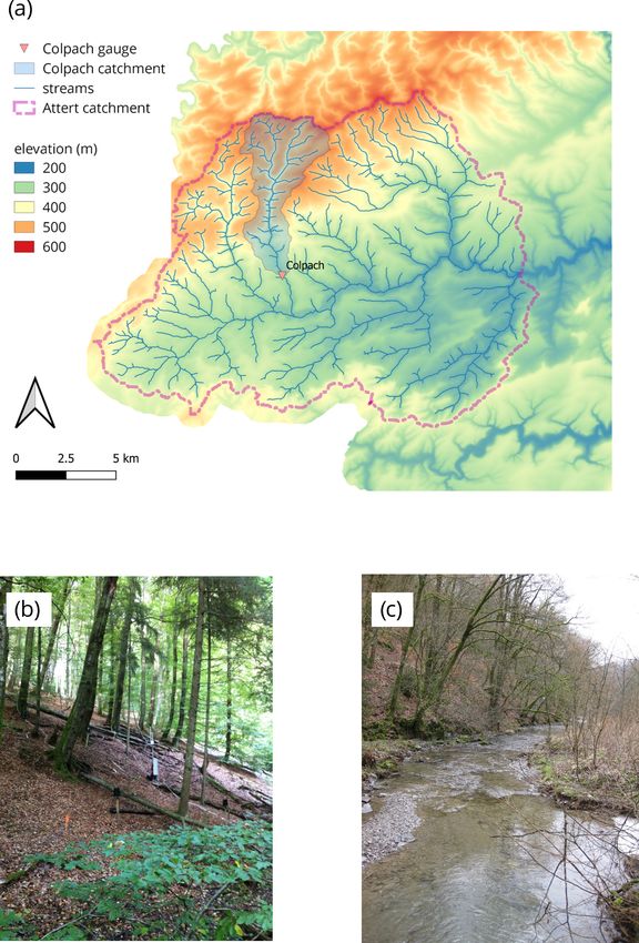
model improve when it is distributed in space and driven Figure 1. (a) Map of the Colpach catchment (location northern Lux-
by distributed rainfall? embourg), (b) picture of a typical forested hillslope within the Col-
pach catchment, and (c) the Colpach River around 4 km north of the
2. Can adaptive clustering be used to distribute a bottom- gauging station.
up model in space that it is able to represent relevant
spatial differences in the system state and precipitation
forcing at the least sufficient resolution to avoid being
ter season), while the runoff generation has a distinct sea-
highly redundant as a fully distributed model?
sonal pattern as around 80 % of the annual discharge is re-
leased between October and March (Seibert et al., 2017). The
2 Study area, hydrological model, and meteorological Colpach and its sub-catchments (e.g., Weierbach) have been
data used as study area in a series of scientific publications. We
refer here to Pfister et al. (2018), Jackisch (2015) or Loritz
2.1 The Colpach catchment et al. (2017) for a more detailed system description (mean
annual precipitation: 900–1000 mm yr−1 ; mean annual evap-
The 19.4 km2 Colpach catchment is located in northern Lux- otranspiration: 450–550 mm yr−1 ; mean annual discharge:
embourg and is a headwater catchment of the 256 km2 large 450–550 mm yr−1 ; land use: 65 % forest, 23 % agriculture,
Attert experimental basin (Fig. 1). The prevailing geology of 2 % others; mean annual temperature: 9.1 ◦ C).
both catchments is Devonian schists of the Ardennes mas-
sif which are characterized by coarse-grained and highly 2.2 The CATFLOW model
permeable soils (> 1 m; e.g., Jackisch et al., 2017; Juilleret
et al., 2011). The steep hills of the Colpach are primar- The key elements of the CATFLOW model (Maurer, 1997;
ily forested, and the elevation of the Colpach ranges from Zehe et al., 2001) are 2D hillslopes which are discretized
265 to 512 m a.s.l. Annual runoff coefficients varied around along a two-dimensional cross section using curvilinear or-
50 % ± 7 % for the 2011–2017 period. Precipitation is rather thogonal coordinates. Evapotranspiration is represented us-
evenly distributed across the seasons (vegetation and win- ing an advanced SVAT (soil–vegetation–atmosphere trans-
https://doi.org/10.5194/hess-25-147-2021 Hydrol. Earth Syst. Sci., 25, 147–167, 2021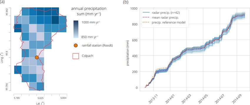
150                             R. Loritz et al.: The role and value of distributed precipitation data in hydrological models

fer) approach based on the Penman–Monteith equation,                 2.4   Spatially resolved precipitation data
which accounts for tabulated vegetation dynamics, albedo as
a function of soil moisture, and the impact of local topog-          Besides the precipitation data from the ground station lo-
raphy on wind speed and radiation. Soil water dynamics are           cated in Roodt, we use a gridded quantitative precipitation
simulated based on the Darcy–Richards equation (solved im-           estimate, which is a merged product of two weather radars,
plicitly, modified Picard iteration; Celia et al., 1990), and sur-   rain gauges, micro rain radars, and disdrometer observations
face runoff is represented by a diffusion wave approximation         (location of the ground measurements in the Supplement
of the Saint-Venant equations using adaptive time stepping           and in more detail in Neuper and Ehret, 2019). The two
(solved explicitly, Euler forward starting downslope). Verti-        radar stations used are located 40 to 70 km and 24 to 44 km
cal and lateral preferential flow paths are represented as con-      away, respectively, from the borders of the Attert catchment
nected pathways containing an artificial porous medium with          (Neuheilenbach, Germany; Wideumont, Belgium) and are
high hydraulic conductivity and very low retention. The hills-       operated by the German Weather Service (DWD) as well
lope module is designed to simulate infiltration excess runoff,      as by the Royal Meteorological Institute of Belgium (RMI).
saturation excess runoff, re-infiltration of surface runoff, lat-    Both distances are within a range that the data can be used
eral water flow in the subsurface, and return flow but can-          at a high resolution of 1 × 1 km as the signal is neither de-
not handle snowfall or snow accumulation. The latter means           graded by beam spreading nor impacted by partial blindness
that CATFLOW should not be applied if snow is a domi-                through cone of silence issues (Neuper and Ehret, 2019). The
nant control, which is not the case in the Colpach catch-            raw data, 10 min reflectivity data from single polarimetric C-
ment. The model core is written entirely in FORTRAN77,               Band Doppler radar, were aggregated to hourly averages and
and the individual hillslopes can be run in parallel on differ-      filtered by static, Doppler clutter filters and bright-band cor-
ent CPUs to assure low computation times and high perfor-            rection following Hannesen (1998). Second trip echoes and
mance of the numerical scheme. Up-to-date model descrip-             obvious anomalous propagation echoes were manually re-
tions can be found in Wienhöfer and Zehe (2014) or in Loritz         moved, and the corrected data were used to create a pseudo
et al. (2017).                                                       plan position indicator data set at 1500 m above the ground.
                                                                     A more detailed description of how the reflectivity data were
2.3   Meteorological forcing and observed discharge                  transformed to rainfall data and calibrated as well as vali-
                                                                     dated against rain gauges, micro rain radars, and disdrom-
Meteorological input data used here are recorded at a tem-           eters can be found in the Supplement and in Neuper and
poral resolution of 1 h at two official meteorological sta-          Ehret (2019).
tions by the “Administration des Services Techniques de                  The chosen precipitation time series starts on 1 Octo-
l’Agriculture Luxembourg” at the locations Roodt and Usel-           ber 2013 and ends on 30 September 2014. 42 grid cells
dange. The meteorological station Roodt measures rainfall            (1 × 1 km) of the precipitation field intersect with more than
within the catchment border (Fig. 2a) and provided the pre-          50 % of their area with the Colpach catchment and are used
cipitation input to the model of Loritz et al. (2017). The sec-      in this study (Fig. 2a). The weather radar measured an area-
ond station Useldange, located outside the catchment around          weighted mean of around 900 mm yr−1 in the Colpach catch-
8 km west of the Colpach outlet, measures air temperature,           ment for the selected period. This is in accordance with the
relative humidity, wind speed, and global radiation. These           reported climatic averages (900–1000 mm yr−1 ) of this re-
data are used as meteorological input (except for precipita-         gion (Pfister et al., 2017). The maximum hourly precipita-
tion) in all model setups in this study. In other words, this        tion difference between the grid cells in the study period is
means that all model setups in this study are forced by iden-        14 mm h−1 (August 2014), and the maximum annual pre-
tical meteorological inputs, except for the precipitation data       cipitation difference between the grid cells is 95 mm yr−1
(see Sect. 3.1). Therefore, we cannot account for variations of      (Fig. 2b). Temporally, the precipitation distributes evenly
the wind speed or the temperature within the Colpach catch-          over the year, with around 50 % of rainfall in winter and 50 %
ment. A detailed description and analysis of the meteorolog-         of rainfall in summer with a short dry spell from mid-March
ical data can be found in Loritz et al. (2017).                      to the end of April. There is a weak correlation between the
   Discharge observations of the Colpach are provided                mean elevation of the grid cells and the annual precipita-
by the Luxembourg Institute of Science and Technol-                  tion sums of 0.43. This implies that precipitation tends to
ogy (LIST) in a 15 min temporal resolution for the hydro-            be slightly higher in the northern parts of the catchment that
logical year 2013/14. The data were aggregated to an hourly          are also characterized by higher altitudes (Fig. 2a). The mea-
temporal resolution and to specific discharge given the catch-       sured precipitation time series from the ground station lo-
ment area of 19.4 km2 .                                              cated in Roodt differs from the mean precipitation of the spa-
                                                                     tial rainfall field about 30 mm yr−1 and around 60 mm yr−1
                                                                     from the exact location in the precipitation grid measured by
                                                                     the weather radar, with a tendency of higher rainfall values
                                                                     especially in the winter season. Why exactly the precipitation

Hydrol. Earth Syst. Sci., 25, 147–167, 2021                                            https://doi.org/10.5194/hess-25-147-2021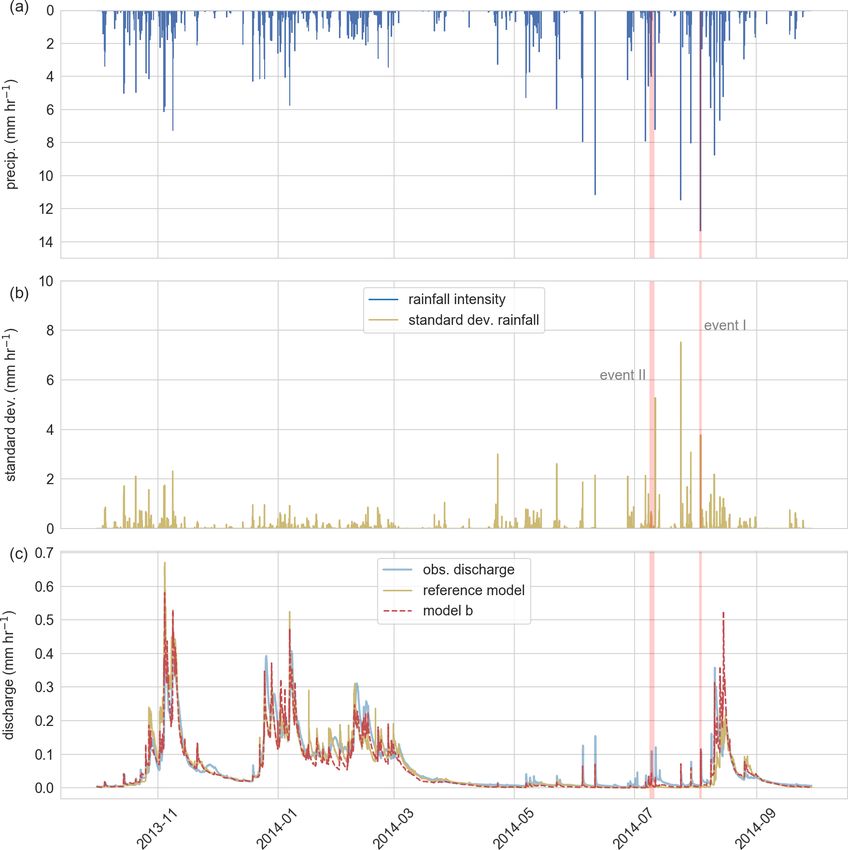
R. Loritz et al.: The role and value of distributed precipitation data in hydrological models                                            151

Figure 2. Annual sums of the gridded precipitation field over the Colpach catchment for the hydrological year 2013/14 as well as the
location of the rainfall station Roodt, which is used as precipitation input for the reference model (spatial resolution: 1 km2 ; coord. sys-
tem WGS84) (a). Cumulated precipitation for each grid cell for the hydrological year 2013/14 of the precipitation field (blue lines), the
corresponding mean of the precipitation field (dashed red line) and the precipitation data from the station in Roodt (b, dashed orange lines).

observations of the ground station in Roodt differ in this mag-          against discharge observations from a sub-basin of the Col-
nitude from the merged product of the weather radar is an                pach, in a different hydrological year, against hourly soil
interesting research question, however, not within the scope             moisture observations (38 sensors in 10 and 50 cm depth),
of this study.                                                           and with hourly normalized sap flow velocities (proxy for
                                                                         transpiration; 30 sensors). The developed model structure
                                                                         agreed well with the dynamics of the observables and showed
3     Modeling approach                                                  higher model performances as reported in other studies work-
                                                                         ing with different top-down model setups in the same envi-
In Sect. 3.1 to 3.3, we introduce three non-adaptive model se-           ronment (Wrede et al., 2015).
tups (reference model, model a, and model b) and a spatially                To summarize, the reference model serves as a benchmark
adaptive model setup (model c). Details on how the model                 here to (a) evaluate the other models and (b) provide the
setups are tested are provided in Sect. 3.4 and 3.5. A sum-              structural basis for them. None of the other model setups are
mary of the different model setups can be found in Table 1.              further calibrated or manually tuned, and the only difference
                                                                         between the different model setups is the precipitation data
3.1    The reference model of Loritz et al. (2017)                       they are driven with and their model resolution. For further
                                                                         details on how the reference model was set up and tuned, we
All model setups in this study are based on a spatially ag-
                                                                         refer to the study of Loritz et al. (2017).
gregated model structure (reference model), developed and
extensively tested in the Colpach catchment in a previous
study (Loritz et al., 2017). The general idea behind the pro-            3.2    Non-adaptive models a and b
posed model concept (representative hillslope) is that a sin-
gle bottom-up hillslope model reflects a meaningful com-                 Despite the acceptable annual model performance of the ref-
promise between classical top-down and bottom-up models                  erence model, it showed deficits in simulated runoff response
(Hrachowitz and Clark, 2017; Loritz, 2019). This is because              to a series of summer rainfall-runoff events. As discussed in
a representative hillslope resolves the effective gradient and           Loritz et al. (2017), one possible explanation for the unsat-
resistance controlling water storage and release and allows              isfying performance is that summer precipitation in the Col-
macroscopic model parameters to be derived from available                pach catchment is mainly driven by convective atmospheric
point measurements. The parameters of the model of Loritz                conditions. These convective precipitation events are charac-
et al. (2017) were, for the most part, derived directly from             terized by a much smaller spatial extent as well as by higher
a large amount of field data, and the model was only man-                rainfall intensities compared to the stratiform and frontal pre-
ually fine-tuned afterwards by further exclusively adjusting             cipitation events that dominate during winter (Neuper and
the spatial macropore density within a few trial and error               Ehret, 2019). The insufficient model performance in summer
runs to simulate the seasonal water balance of the Colpach               could therefore likely be a consequence of the larger spatial
catchment. The model simulations were tested against hourly              gradients of the rainfall field compared to the winter season
discharge observations on an annual and seasonal timescale,              that cannot be accounted for in the original model of Loritz et

https://doi.org/10.5194/hess-25-147-2021                                                  Hydrol. Earth Syst. Sci., 25, 147–167, 2021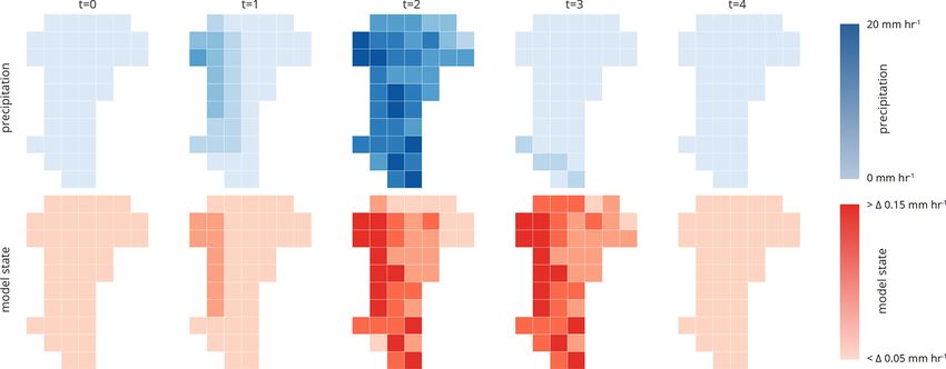
152                               R. Loritz et al.: The role and value of distributed precipitation data in hydrological models

Table 1. Summary of the four different model setups.

                                   Reference model     Spatially aggregated      Spatially distributed   Spatially adaptive
                                                       model a                   model b                 model c
                  Spatially        no                  no                        yes                     yes
                  distributed:
                  Precipitation    single precip.      single precip.            distributed             binned distri.
                  forcing:         time series         time series               precip.                 precip.
                                   (ground station)    (weather radar)           (weather radar)         (weather radar)
                  Spatially        no                  no                        no                      yes
                  adaptive:
                  Testing          hydro. year         hydro. year               hydro. year             rainfall event
                  period:          2013/14, summer     2013/14, summer           2013/14, summer         I and II
                                   season, rainfall    season, rainfall          season, rainfall
                                   event I and II      event I and II            event I and II

al. (2017). In other words, this necessitates that a hydrologi-          3.2.2    Spatially distributed model b
cal model, distributed at a sufficiently high spatial resolution,
is required to capture the spatial variability of the precipita-         Model b is a spatially distributed version of the reference
tion field to achieve improved simulations of the runoff gen-            model. More specifically, here all model parameters of the
eration of the Colpach. One goal of this study (first research           representative hillslope (reference model), as well as all other
question) is hence to test the hypothesis as to whether the per-         meteorological variables such as temperature or wind speed,
formance deficiencies of the representative hillslope model,             are identical to the reference model. However, model b is
the reference model, in summer are mainly caused by the in-              spatially distributed as well as driven by distributed rainfall
ability of the setup to account for the spatial variability of the       data. This model setup is distributed on the spatial resolution
precipitation field.                                                     of the precipitation field similarity, as done for instance by
   To address the first research questions of this study (“Does          Prenner et al. (2018) and not following the traditional spatial
the model performance of a spatially aggregated model im-                discretization strategy of CATFOW based on a fixed number
prove if it is distributed in space and driven by distributed            of hillslopes, inferred from surface topography or land use.
rainfall”), we analyze simulations of two alternative model              Model b thus represents the Colpach with 42 spatial grids
setups (model a and model b), additional to the reference                (1 × 1 km). In each of these grids, we run a model identical
model from Loritz et al. (2017). Both model setups are de-               to the reference model, however, driven with the specific pre-
scribed in detail below.                                                 cipitation data measured at this location.
                                                                            We justify this assumption based on the model validation
3.2.1   Spatially aggregated model a                                     in Loritz et al. (2017) and on a study conducted in the same
                                                                         research environment (Loritz et al., 2019), where we showed
Model a is structurally identical to the reference model; how-           that different sub-basins of the Attert catchment (the Colpach
ever, it is driven by the area-weighted mean of the spatially            is a headwater catchment of the Attert catchment) have simi-
resolved precipitation data described in Sect. 2.4 and plotted           lar specific discharges as long as they are located in the same
in Fig. 2b. We used the area-weighted mean as not all raster             geological setting and are driven by a similar meteorological
cells of the distributed precipitation data are entirely within          forcing (see also Sect. 4.2).
the borders of the Colpach catchment. This means that the
weight of a grid cell which is not entirely located within the           3.3     Spatially adaptive model c
catchment is reduced when we calculate the average accord-
ing to the percentage areal overlap.                                     To address the second and main research question of this
   We added model a to test if the performance difference                study (“Can adaptive clustering be used to distribute a
between the reference model and our distributed model b is               bottom-up model in space that it is able to represent rel-
merely a result of quantitative differences between the differ-          evant spatial differences in the system state and precipita-
ent precipitation products measured either by a single ground            tion forcing at the least sufficient resolution to avoid being
station or by a weather radar in combination with different              highly redundant as a fully distributed model?”), we develop
ground stations.                                                         a third adaptive model setup (model c). This spatially adap-
                                                                         tive model setup is based on the distributed model b, how-
                                                                         ever, is able to dynamically adjust its spatial structure in time

Hydrol. Earth Syst. Sci., 25, 147–167, 2021                                                   https://doi.org/10.5194/hess-25-147-2021
R. Loritz et al.: The role and value of distributed precipitation data in hydrological models 153
based on the precipitation forcing, as detailed in Sect. 4.1 duced number of hillslopes (coarser resolution). We therefore
to 4.3. calculate not only the KGE between the simulated discharge
of model c with the observed discharge at event I and II but
3.4 Model testing – non-adaptive models a and b also the KGE between the simulated discharge of model c
and the simulated discharge of model b on an hourly basis. A
We analyze the simulation performances of model a (spa- full automation of the proposed adaptive clustering approach
tially aggregated) and b (spatially distributed) by calculating and a test on a longer timescale are beyond the scope of this
the Kling–Gupta efficiency (KGE; Kling and Gupta, 2009) study, and we point towards the study of Ehret et al. (2020),
and analyze its three components (see Supplement) between who have shown the potential of adaptive clustering using a
the hourly discharge simulations of the individual model se- conceptual model, also for longer periods.
tups against hourly observed discharge at different timescales
(annual, seasonal, event scale). Model a and b are run for the
hydrological year 2013–2014 with hourly printout times and 4 Spatially adaptive modeling
differ only concerning the precipitation data they are driven
with: Spatially adaptive modeling or adaptive clustering is an ap-
proach to dynamically adjust the spatial structure of a hy-
– model a: driven by an area-weighted mean of the spa- drological model in time, offering the possibility to reduce
tially resolved precipitation data; computational times as well as to find an appropriate, time-
– model b: driven by 42 precipitation time series, each varying spatial model resolution (Ehret et al., 2020). The ba-
reflecting a grid cell of the precipitation field shown in sic idea of adaptive clustering has been motivated within the
Fig. 2. work of Zehe et al. (2014), who stated that functional similar-
ity in a catchment (or in a model) can only emerge if different
To be able to compare the discharge of the spatially aggre- sub-units are structurally similar (e.g., topography, geology,
gated model a and the distributed model b with the observed land use), are driven by a similar forcing, and are at a simi-
discharge of the Colpach catchment and to account for the lar state. The latter implies that the concept of hydrological
routing of the water from a specific location to the outlet, we similarity, frequently used as the basis to discretize a catch-
added a simple lag function acting as the channel network. ment in space (e.g., Sivapalan et al., 1987), cannot be time-
The latter is based on the average flow length along the sur- invariant but needs to dynamically change in time (Loritz et
face topography of each precipitation grid to the outlet of al., 2018). This is the case as the relevance of different spa-
the catchment assuming a constant flow velocity of 1 m s−1 tial controls like the topography or pedology of a catchment
(e.g., Leopold, 1953). The flow length of each grid is esti- depends on the prevailing state and forcing (Woods and Siva-
mated based on a 10 m resolved digital elevation model. For palan, 1999). A suitable discretization of a catchment into
the spatially aggregated model a, we average all flow dis- similar functional units needs hence to be time-variant, and
tances to the outlet and shift the single discharge simulation one way to achieve such a dynamic model resolution is spa-
accordingly. tially adaptive modeling.
Implementing adaptive clustering into a distributed model
3.5 Model testing – adaptive model c requires specific decision thresholds that define whether spa-
tial differences in the structure, forcing, and state of sub-
We test the spatially adaptive model c for two selected
units (e.g., hillslopes, sub-basins) are so large that they need
rainfall-runoff events, which are characterized by distinctly
a distributed representation. This means that if differences
different precipitation properties. We chose event I as it has
between the structure, forcing, or state of two or more dis-
the highest intensity and third-highest spatial variability in
tributed model elements (here gridded models) are below
summer and event II because it is the event with the longest
these thresholds they are by definition similar, which means
continuous precipitation in the time series. Both events were
that they can represent each other’s hydrological function.
picked to represent the spectrum of rainfall events in the
The concept that certain spatial model elements can repre-
summer season. We focus exclusively on the summer sea-
sent other model elements is not new and has been used fre-
son as the distributed model b only outperforms the refer-
quently in hydrology since at least Sivapalan et al. (1987),
ence model in this period, indicating that spatially distributed
who introduced the concept of representative elementary ar-
rainfall provides no performance-relevant information during
eas. The novelty of adaptive clustering is that hydrological
winter. A full automation of the proposed adaptive clustering
similar model elements are dynamically grouped and split in
approach is beyond the scope of this study, and we focus here
the runtime of the model instead of running a constant num-
on the introduction as well as the physical underpinning of
ber of model elements for the entire simulation period (Ehret
the approach.
et al., 2020).
The main goal of testing the spatially adaptive model c is
to show that we can achieve similar simulation results com-
pared to the fully distributed model b, however, with a re-
https://doi.org/10.5194/hess-25-147-2021 Hydrol. Earth Syst. Sci., 25, 147–167, 2021154 R. Loritz et al.: The role and value of distributed precipitation data in hydrological models
4.1 Spatially adaptive modeling – similarity 4.1.2 Time-variant similarity of the precipitation
assumption forcing
Identifying periods when a model element can represent an- The second decision threshold we need to identify defines
other one because it functions hydrologically similarly is the the minimum difference at which we consider differences in
main challenge of adaptive clustering. For this purpose, we the precipitation field as relevant for the runoff generation.
subdivide the precipitation field and the model states at each Simply speaking, two structurally similar hydrological units
time step into equally distant bins (bins = groups) and clas- that are in the same state will only respond differently to an
sify those as similar that occupy the same bin. If two or more external forcing if the variability in the forcing has exceeded
observations or models are hence in the same bin, they are this threshold. Here, we picked a threshold of 1 mm h−1 upon
by our definition functionally similar and can represent each which we consider differences between precipitation obser-
other. To give an example, imagine if 50 % of the catchment vations (grid cells) as relevant. We chose this threshold as a
area receives precipitation of around 1 mm h−1 and 50 % reasonable value for which we expect differences in hydro-
around 2 mm h−1 . In this specific case, we would have two logic behavior in this humid catchment and based on our col-
occupied forcing bins (precipitation groups; PB). In the fol- lective understanding of the Colpach catchment. This means
lowing, we explain how we have chosen the decision thresh- that only if the spatial differences in the precipitation field are
olds for the system structure, the precipitation forcing, and above 1 mm h−1 do we drive the spatially adaptive model c
the model states. with different precipitation inputs. The choice of this thresh-
old is important, as it is one of two main controls or param-
4.1.1 Time invariant similarity of the system structure eters of the model resolution of the spatially adaptive model
(see Supplement B).
The first step of our adaptive clustering approach requires the
identification of hydrological response units (HRUs) that po-
4.1.3 Time-variant similarity of the catchment state
tentially behave similarly. These similar units are typically
identified based on structural properties such as the geologi-
The third assumption is to identify a decision threshold upon
cal setting, the land use, or the topography. The general idea
which we consider that two model elements are in the same
is that HRUs are grouped together which share the same con-
state. This means that we need to select a point in time after
trols on gradients and resistances controlling flows of water
a spatially variable rainfall event (> 1 mm h−1 ) when two or
as long as they are in the same state (Zehe et al., 2014). As
more model elements in the individual grid cells have dissi-
already mentioned in Sect. 3.2, our previous studies showed
pated the differences between them introduced by the previ-
that different sub-units of the Colpach catchment are charac-
ous precipitation input with drainage and evapotranspiration
terized by similar spatially organized surface and subsurface
dynamics. Here, we use the change in discharge over time
characteristics (integral filter properties). This entails a po-
(dQ dt −1 ; slope of the simulated hydrograph) and the dis-
tential similar rainfall-runoff transformation when they are in
charge (Q) at a time step to infer similar model states. By
a similar state. The latter is supported by our previous work
that, we expect that two or more gridded models are again
(Loritz et al., 2017, 2019), which revealed that a sub-basin of
in the same state if the individual models estimate runoff and
the Colpach catchment (0.45 km2 ) and a neighboring catch-
the slope of the runoff within a 0.05 mm h−1 margin. As soon
ment (30 km2 ) located in the same geological setting have
as this is the case and two or more gridded models are in
almost identical specific discharges as long as they are at
the same state, we average their states (average saturation of
similar states and forced by comparable amounts of precip-
each grid cell of the CATFLOW hillslope grid) and, by that,
itation. We hence assume that all grid cells of the precipi-
aggregate the models back again into a one hillslope. The
tation field can thus be represented by the same model with
value of 0.05 mm h−1 for Q and dQ dt −1 was picked as it
the same model parameters as long as they are in the same
reflects the desired precision of the adaptive model c. Similar
state and driven by the same forcing. This necessitates, how-
to the case of the decision threshold, this value needs to be
ever, also that if we extend our research area to a catchment
picked carefully. Furthermore, it is important to choose simi-
that is divided, for instance, into two or more geological set-
larity metrics (here dQ dt −1 and Q) that adequately describe
tings and different dominant land use or soil types that func-
the model states during the simulation time.
tion hydrologically differently (regarding their integral filter
properties), we need to run two or more structurally different
4.2 Spatially adaptive modeling – model
models. Each of these models represents thereby a unique
implementation
structural setting. The latter might limit the possibilities to
apply this approach on larger scales or in areas with complex
As stated in Sect. 3.1, we classified the entire Colpach catch-
structural settings.
ment as hydrologically similar with respect to the runoff gen-
eration as long as the different hydrological sub-units of the
catchment are in the same state and receive a comparable
Hydrol. Earth Syst. Sci., 25, 147–167, 2021 https://doi.org/10.5194/hess-25-147-2021R. Loritz et al.: The role and value of distributed precipitation data in hydrological models 155
sions. In the case that the hillslopes are not structurally simi-
lar, this requires a weighted averaging of soil water contents
to avoid a violation of mass conservation. After the aggrega-
tion of the two models, we have two model states left (S = 2),
each representing 50 % of the catchment area.
If no further rainfall occurs, we wait until the gradients in
system states are depleted and the two running models have
“forgotten” the difference in the past forcing, and both pre-
dict similar dQ dt −1 and Q values and eventually aggregate
the two models to one hillslope model. If rainfall is continu-
ous in the next time step (PB > 1), we need to check which
model states (S) receive which forcing. For instance, given
our hypothetical example, we know that after the last simu-
lation step we needed two model states (S = 2) to represent
Figure 3. Sketch of the spatial adaptive modeling described in our catchment. Each of these two states represents 50 % of
Sect. 4.2. The upper panel shows the precipitation forcing (blue) the area of the catchment. Imagine that at the next time step
and the lower panel the model states (red). The numbers below the we observe a precipitation event, in which 50 % of the catch-
figures indicate how many precipitation (PB) and model state (S) ment receives 8 mm h−1 and the other 50 % 3 mm h−1 (Fig. 3,
bins (groups) are occupied and how many models (M) are running
t = 2). In this case, we have to check if the two model states
at the given time step.
(S = 2) receive both precipitation inputs of 8 and 3 mm h−1 .
Let us assume that one model state receives 80 % of the
8 mm h−1 and 20 % of 3 mm h−1 rainfall and the other model
forcing. This means that we start the simulation with one 20 % of the 8 mm h−1 and 80 % 3 mm h−1 . In this specific
gridded hillslope to represent the entire catchment and con- setting, we would need to run four models (M = 4) to ac-
tinue in this mode as long as we have not detected a spatial count for the spatial variability of the model states and pre-
difference in the precipitation field above the selected thresh- cipitation input, while each of those reflect a different com-
old of 1 mm h−1 (Fig. 3, t = 0). At each time step, we bin bination of the model state and forcing in different parts of
the precipitation input of the next time step and determine the catchment. At this stage, we again either wait until the
the number of allocated bins (PB is the number of precipi- internal differences have been dissipated to reduce the num-
tation bins). If more than one precipitation bin is occupied ber of models, or we increase the number of models in the
(PB > 1), we increase the number of gridded models (M is case that the precipitation with larger spatial variability of
the number of running gridded models) by running the same PB = 1 continues (Fig. 3, t = n). The maximum number of
model in the same initial state, however, driven by different models we could require in our adaptive clustering approach
precipitation inputs. depends on the maximum number of precipitation grid cells
Consider a scenario in which the Colpach catchment (42 in this study). The highest resolution that the spatially
is represented by one hillslope (S = 1), and we observe adaptive model c can reach in this study is reflected by the
a precipitation event in which 50 % of the catchment re- spatially distributed model b.
ceives no precipitation, 20 % 7 mm h−1 and 30 % 8 mm h−1 ,
as displayed in an illustrative example in Fig. 3 at t = 1. 4.3 Spatially adaptive modeling – model analysis
This would mean that three precipitation bins are allocated
(PB = 3), and we need to increase the number of running To test our spatially adaptive model c against the observed
models to three (M = 3). After running these three models discharge of the catchment, we route the simulated runoff
for one time step with the different precipitation inputs, we contributions according to their location to the outlet by as-
bin the model states (dQ dt −1 ; Q). Let us assume we would suming a mean flow velocity of water within the channel
identify two occupied model state bins, which means that network of 1 m s−1 . However, as the same model can rep-
two different model states (S = 2) are needed to represent the resent different grids with different locations, we addition-
spatial variability of catchment states. This could happen if ally need to calculate the average flow distances to the outlet
the differences between the 7 and 8 mm h−1 rainfall intensity of all grids a model is representing and shift the simulation
did not result in a significant difference in the discharge sim- by the average distance accordingly. We then take the area-
ulation of the two corresponding models. Following our ap- weighted mean of every simulation at each time step. The
proach, we aggregate the two models that are driven by 7 and performance of the adaptive model c is then quantified by the
8 mm h−1 by averaging their states. We do this by averaging KGE against the observed discharge and the area-weighted
the relative saturation of the corresponding CATFLOW hill- average of the distributed model b. The latter addresses our
slope grids. The latter is straightforward in our study as they second research question and follows the logic that a suitable
have the same width as well as lateral and vertical dimen- adaptive modeling approach should lead to similar simula-
https://doi.org/10.5194/hess-25-147-2021 Hydrol. Earth Syst. Sci., 25, 147–167, 2021156 R. Loritz et al.: The role and value of distributed precipitation data in hydrological models
tions as a fully distributed model, however, with fewer model rainfall intensity of 19 mm h−1 and the third-highest spatial
elements. While we use CATFLOW as a model here, the pro- variability estimated by the standard deviation of 3.8 mm h−1
posed approach is not restricted to this model and can be in the time series as well as a distinct runoff reaction. Rainfall
used in any hydrological model framework that distributes event I was observed at the beginning of August and lasted
a catchment into independent spatial units. One advantage of for about 5 h, and the highest spatial differences between the
CATFLOW (or similar type of models) is that it also uses an grid cells of 14 mm h−1 was reached right at the beginning
adaptive time step procedure, making the final model adap- of the event (Figs. 5 and 6). The rainfall event I moved from
tive in space and time. However, if a model represents a land- west to east over the catchment and reached its maximum
scape in an entirely continuous manner without a delineation rainfall intensity after 3 h. No rainfall had occurred before
of the landscape into independent sub-units like several 2D the event for a period of 102 h. It can hence be assumed that
surface runoff models, an adaptive mesh (numerical grid) is the catchment was in a moderately dry state before the event,
required in case the spatial resolution should adapt itself dur- also indicated by soil moisture measurements presented in
ing runtime. Loritz et al. (2017).
The second rainfall event was selected as it has distinctly
different properties (low spatial variability, low intensity,
5 Results longer duration) as compared to the first event. Event II has
a maximum rainfall intensity of 5.8 mm h−1 and a maximum
In the following section, we investigate the precipitation field spatial difference between the grid cells of 4 mm h−1 . The
and compare the performance of the discharge simulations event lasted for around 15 h, making it the longest continu-
of the reference model, the spatially aggregated model a, ing rainfall in the summer season, and there was no rainfall
and distributed model b at the annual, seasonal, and event observed 20 h before the event but more than 36 mm of rain-
scale by comparing hourly simulations against hourly ob- fall over the preceding 3 d. It seems hence reasonable to as-
served discharge. We furthermore present the simulation re- sume that the soils in the catchment were rather wet, which is
sults of the adaptive model c for two selected rainfall events, again supported by the soil moisture measurements presented
including the spatial distribution of the precipitation and the in Loritz et al. (2017).
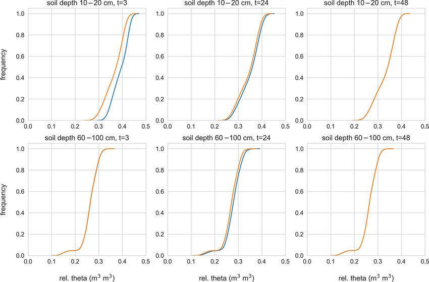
model states. Finally, we show the soil moisture distribution
of two hillslope models at different time steps that have re- 5.2 Temporal dependency of the model performance
ceived a significant dissimilar precipitation forcing to high-
light the importance of the dissipation timescale for adaptive The performances of the four model setups (reference model
modeling. and model a, b, and c) to simulate the observed discharge of
the Colpach catchment estimated by means of the KGE are
5.1 Precipitation characteristics shown in Table 2. Comparing the two spatially aggregated
models that differ only with respect to their rainfall forcing,
While rainfall sums are equally distributed between the the reference model outperforms model a during the win-
winter (October–March) and vegetation season (April– ter season and on the annual timescale, while model a has
September) in the selected hydrological year 2013/14 a higher performance during the vegetation season (April–
(Fig. 2b), the rainfall intensities and the associated standard September). Both models are characterized by KGE values
deviation (here used to measure the spatial variability of the higher than 0.8 in the winter season and for the entire hydro-
precipitation field) of the precipitation field are in general logical year, while the predictive performance drops in sum-
higher in summer (Fig. 4a and b). For instance, the five rain- mer and is particularly low for the two rainfall-runoff events,
fall events with the highest rainfall intensities and the highest even resulting in negative KGE values. The differences be-
standard deviation in space were all observed in the summer tween the KGE values (1KGE) between the two spatially
season. Rainfall intensity and spatial variability are strongly aggregated models (reference model and model a) are low
linked to each other, which is reflected in their correlation in winter, increase in summer, and are the highest for the
of 0.82. The latter is no surprise as convective storms, which convective rainfall event I. Here model a only has a slightly
dominate the precipitation generation in summer, are typi- improved predictive performance as the average discharge of
cally characterized by higher spatiotemporal variabilities and the event, indicated by a KGE value of −0.16 (please note
higher rainfall intensities. This finding is neither surprising that the performance of the mean of the observation is not
nor limited to the chosen research environment (e.g., Hra- zero as in the case when using the Nash–Sutcliffe efficiency,
chowitz and Weiler, 2011; Wilson et al., 1979), but it con- as shown by Knoben et al., 2019).
firms one of our initial assumptions that rainfall is spatially The observed discharge of the Colpach catchment and the
more diverse in the summer season compared to the winter discharge simulations of the reference model, as well as the
months in the Colpach catchment. discharge simulation of the distributed model b, are presented
We selected two rainfall-runoff events to test the adaptive in Fig. 4c. Visual comparison of the two models shows that
model c (Fig. 4). We chose the first event as it has the highest the reference model has lower runoff production during sum-
Hydrol. Earth Syst. Sci., 25, 147–167, 2021 https://doi.org/10.5194/hess-25-147-2021R. Loritz et al.: The role and value of distributed precipitation data in hydrological models 157
Figure 4. (a) Average rainfall intensity of the precipitation field (mm h−1 ), (b) corresponding standard deviation of the precipitation
field (mm h−1 ), (c) observed discharge of the Colpach catchment and the discharge simulation of the reference model as well as of the
distributed model b. The two red bars display the location of the two selected rainfall-runoff events used to test the adaptive clustering
approach.
Table 2. Model performances of the four model setups to simulate the observed discharge of the Colpach catchment measured using the
Kling–Gupta efficiency (KGE), based on hourly simulation and observation time steps. Performances are shown for the entire hydrological
year (2013/2014), for the winter (October–March) and summer season (April–September), and for two selected summer rainfall-runoff events
in July and August. The three components of the KGE can be found in the Supplement.
Annual Winter Summer Rainfall Rainfall
performance performance performance event I event II
(KGE) (KGE) (KGE) (KGE) (KGE)
Reference model 0.88 0.88 0.52 0.1 −0.2
from Loritz et al. (2017)
Model a 0.85 0.84 0.65 −0.16 −0.05
(spatially aggregated)
Model b 0.91 0.89 0.73 0.29 0.1
(distributed model)
Model c – – – 0.29 0.1
(adaptive model)
https://doi.org/10.5194/hess-25-147-2021 Hydrol. Earth Syst. Sci., 25, 147–167, 2021158 R. Loritz et al.: The role and value of distributed precipitation data in hydrological models Figure 5. Binned precipitation field (blue) and binned model states (orange) of the adaptive model (t = 0; 3 August 2014 15:00 CET). PB is the no. of allocated precipitation bins, S the no. of allocated model space bins, and M the no. of running models at the given time step. The spatial distribution of the precipitation and the model states for event I are displayed in Fig. 6. Figure 6. Spatial and temporal distribution of the precipitation field (upper panel) and the corresponding states of the actual model grids used by the adaptive model c (lower panel). The model state is estimated by the slope of the simulated discharge. The corresponding bins (groups) of the precipitation and model states are shown in Fig. 5. mer, which is particularly visible in August and September. summer season. Overall, model b has the highest predic- Interestingly, the latter cannot be explained by the annual or tive performance as indicated by the KGE in all five test seasonal precipitation sums as both models are driven on av- periods (annual, winter, summer, and the two selected rain- erage by similar precipitation sums of around 900 mm yr−1 fall events) when compared to the two spatially aggregated for the entire year and around 450 mm per 6 months in the models (reference model and model a). The absolute differ- Hydrol. Earth Syst. Sci., 25, 147–167, 2021 https://doi.org/10.5194/hess-25-147-2021
R. Loritz et al.: The role and value of distributed precipitation data in hydrological models                                         159

Figure 7. (a) Rainfall-runoff event I and (b) rainfall-runoff event II. Blue bars in the upper panel show the average precipitation of the
precipitation field for each time step (mm h−1 ). The green curves in the lower panel represent a single gridded model of the distributed
model b, the red line the area-weighted mean of the distributed model, the dashed purple line the area-weighted mean of the adaptive model,
and the dashed blue line the observed specific discharge of the Colpach.

ences between the model performances depend again on the                on the chosen bin width of 1 mm h−1 . The rainfall field allo-
selected period. For instance, for the entire simulation pe-            cates 0 bins (precipitation groups) at t = 0 (PB = 0), 12 bins
riod, the reference model and model b have close to equal               at t = 1 (PB = 12), 13 bins at t = 2 (PB = 13), 3 bins at t = 3
KGE values around 0.9, while the differences between the                (PB = 3), and 2 bins at t = 4 (PB = 2). The number of oc-
KGE values are 1KGE = 0.21 in summer and for the rain-                  cupied bins indicates the spatial variability of the rainfall
fall event II around 1KGE = 0.3.                                        event at a given time step and would reach maximum spa-
   Although model b has the highest KGE values for the                  tial complexity if PB equals 42. This means that if a high
two selected rainfall-runoff events, the general model per-             number of bins is allocated, the forcing is spatially variable
formance is, given the KGE values of 0.29 and 0.1, still rel-           and therefore a higher number of models is needed to repre-
atively low for both runoff events. The low performance can             sent the spatial variability of the precipitation. The number
be explained by a general underestimation of the total runoff           of bins does, however, not specify how large the gradients
volume at both events (Fig. 7), while it seems that the shape           are within the spatial precipitation field. For instance, if 50 %
of the simulated hydrograph is simulated acceptably under-              of a precipitation field is characterized by a rainfall amount
pinned by a correlation of 0.72 and 0.86 between the sim-               of 20 mm h−1 and the other 50 % by 1 mm h−1 , the number
ulation and observation (see Supplement for the three com-              of allocated bins is two, although the absolute difference be-
ponents of the KGE). The latter is supported by the fact that           tween the bins is large.
distributed model b is able to simulate the observed double                The lower panels of Figs. 5 and 6 display the binning of
peak at event I. We furthermore tested the addition of a direct         the model states (S) of the adaptive model for each time step
runoff component by assuming that 10 % of the rainfall is di-           of event I for the similarity measure dQ dt −1 . We do not plot
rectly added to the channel network instead of falling on the           the similarity measure Q here as in our specific case, Q and
hillslopes. This model extension could be justified by sealed           dQ dt −1 lead to the same classification at both events. How-
areas within the catchment or by precipitation that directly            ever, this does not mean that Q is less relevant as in theory
falls into the stream or on saturated areas like the riparian           two models could simulate identical dQ dt −1 values but very
zone. This rather simple model extension increases the KGE              different absolute Q values. This shows that the set of simi-
of model b from 0.29 to 0.48 at event I. However, we do not             larity measures should be picked carefully and depend very
update our model here as the main goal of this study is not to          much on the given modeling task and the research environ-
perform the best possible rainfall-runoff simulation but to in-         ment.
vestigate the role of the spatiotemporal patterns of rainfall in           At t = 0, we run a single model representing the entire
the runoff generation of a mesoscale catchment by introduc-             catchment with a single model state. At t = 1, the precipi-
ing the concept of a spatially adaptive hydrological model.             tation starts, and the spatial field is classified into 12 bins
                                                                        (PB = 12). Following our approach, this necessitates that we
5.3   Spatially adaptive modeling – simulation results                  need to run 12 models (M = 12) at t = 1 to account for the
                                                                        spatial variability of the rainfall. After one simulation step,
The upper panel of Fig. 5 shows the binned precipitation field          we estimate the number of model states by binning the abso-
of rainfall event I. The precipitation field was binned based           lute values (Q) and slope (dQ dt −1 ) of the discharge simula-

https://doi.org/10.5194/hess-25-147-2021                                                 Hydrol. Earth Syst. Sci., 25, 147–167, 2021
You can also read