Estimating mean molecular weight, carbon number, and OM/OC with mid-infrared spectroscopy in organic particulate matter samples from a monitoring ...
←
→
Page content transcription
If your browser does not render page correctly, please read the page content below
Atmos. Meas. Tech., 14, 4805–4827, 2021
https://doi.org/10.5194/amt-14-4805-2021
© Author(s) 2021. This work is distributed under
the Creative Commons Attribution 4.0 License.

Estimating mean molecular weight, carbon number, and OM/OC
with mid-infrared spectroscopy in organic particulate matter
samples from a monitoring network
Amir Yazdani1 , Ann M. Dillner2 , and Satoshi Takahama1
1 ENAC/IIE     Swiss Federal Institute of Technology Lausanne (EPFL), Lausanne, Switzerland
2 Air   Quality Research Center, University of California Davis, Davis, CA, USA

Correspondence: Satoshi Takahama (satoshi.takahama@epfl.ch)

Received: 7 March 2020 – Discussion started: 23 March 2020
Revised: 18 July 2020 – Accepted: 11 August 2020 – Published: 8 July 2021

Abstract. Organic matter (OM) is a major constituent of fine        using different approaches. The results are also consistent
particulate matter, which contributes significantly to degra-       with temporal and spatial variations in these quantities as-
dation of visibility and radiative forcing, and causes adverse      sociated with aging processes and different source classes
health effects. However, due to its sheer compositional com-        (anthropogenic, biogenic, and burning sources). For instance,
plexity, OM is difficult to characterize in its entirety. Mid-      the statistical models estimate higher mean carbon number
infrared spectroscopy has previously proven useful in the           for urban samples and smaller, more fragmented molecules
study of OM by providing extensive information about func-          for samples in which substantial aging is anticipated.
tional group composition with high mass recovery. Herein,
we introduce a new method for obtaining additional charac-
teristics such as mean carbon number and molecular weight
of these complex organic mixtures using the aliphatic C−H           1     Introduction
absorbance profile in the mid-infrared spectrum. We apply
this technique to spectra acquired non-destructively from           1.1    Organic aerosols and measurement methods
Teflon filters used for fine particulate matter quantification
at selected sites of the Inter-agency Monitoring of PRO-            Organic matter (OM) is known to be an important constituent
tected Visual Environments (IMPROVE) network. Since car-            of fine particulate matter (PM). It is estimated to consti-
bon number and molecular weight are important character-            tute 20 %–50 % of the total fine PM at midlatitudes and up
istics used by recent conceptual models to describe evolu-          to 90 % in tropical forests (Kanakidou et al., 2005). This
tion in OM composition, this technique can provide semi-            organic fraction contributes significantly to aerosol-related
quantitative, observational constraints of these variables at       phenomena such as visibility and climate change, through
the scale of the network. For this task, multivariate statistical   radiative forcing and affecting cloud formation, and causes
models are trained on calibration spectra prepared from at-         adverse health effects (Shiraiwa et al., 2017b; Hallquist et al.,
mospherically relevant laboratory standards and are applied         2009). Such effects underscore the importance of better
to ambient samples. Then, the physical basis linking the ab-        quantification of organic fraction in particulate matter, which
sorbance profile of this relatively narrow region in the mid-       is a complex mixture of a multitude of compounds whose
infrared spectrum to the molecular structure is investigated        compositions, concentrations, and formation mechanisms are
using a classification approach. The multivariate statistical       not yet completely understood (Turpin et al., 2000).
models predict mean carbon number and molecular weight                 The determination of organic aerosol composition in-
that are consistent with previous values of organic-mass-to-        volves a large range of analytical and computational tech-
organic-carbon (OM/OC) ratios estimated for the network             niques. Among the widely known techniques are gas
                                                                    chromatography/mass spectrometry (GC/MS), mid-infrared

Published by Copernicus Publications on behalf of the European Geosciences Union.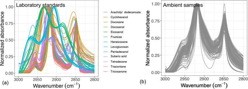
4806                                A. Yazdani et al.: Mean carbon number and molecular weight in atmospheric aerosols

spectroscopy – often referred to as Fourier transform in-           OM. This ability of mid-infrared spectroscopy has been in-
frared spectroscopy (FT-IR) – and aerosol mass spectrometry         vestigated to a lesser extent in the context of atmospheric
(AMS). GC/MS provides molecular speciation information              OM. In this work, we used this aspect to investigate two
but is limited to a small mass fraction of the organic aerosols     important structural parameters in OM, i.e., mean molecular
as low as 10 % (Hallquist et al., 2009). AMS and FT-IR,             weight, and mean carbon number. These two parameters are
however, can be used to analyze most of the organic mass            important characteristics used by recent conceptual models
in addition to providing information about either chemical          and parameterizations to describe evolution in atmospheric
classes or functional groups (Hallquist et al., 2009). AMS          OM, in terms of its volatility and phase state (Shiraiwa et al.,
is an online technique with a relatively high size and time         2017a; Pankow and Barsanti, 2009; Kroll et al., 2011; Don-
resolution. Nevertheless, the extensive fragmentation caused        ahue et al., 2011). Moreover, inspecting the spatial and tem-
by commonly used ionization method in AMS, i.e., electron           poral variations of these parameters helps us understand the
impact (EI) ionization, makes the identification of original        processes involved in aerosol aging, especially fragmentation
species difficult (Canagaratna et al., 2007; Faber et al., 2017).   (Murphy et al., 2012), and can be useful for identification
In recent years, soft ionization methods such as electrospray       of the dominant sources (Price et al., 2017; Gentner et al.,
ionization (ESI), photoionization (PI), and chemical ioniza-        2012).
tion (CI) have been used frequently for predicting physico-            In this paper, the mean molecular weight, carbon num-
chemical properties of organic aerosol (OA), e.g., volatility       ber, and OM/OC ratio of ambient aerosols, which were col-
(Li et al., 2016; Xie et al., 2020), phase state, and viscos-       lected on polytetrafluoroethylene (PTFE) filters at selected
ity (Li et al., 2020; DeRieux et al., 2018; Shiraiwa et al.,        Inter-agency Monitoring of PROtected Visual Environments
2017a), as a function of measured elemental composition             (IMPROVE) sites, were estimated using FT-IR spectroscopy.
and molecular weight. These methods minimize analyte frag-          First, the aliphatic C−H region (2800–3000 cm−1 ) was ex-
mentation, providing better estimates of molar mass of in-          tracted from the baseline-corrected spectra of laboratory
dividual molecules but often have other shortcomings such           standards. The C−H spectral bands were then normalized to
as ionization efficiency, which varies by molecule (Nozière         eliminate abundance information. Then, partial least squares
et al., 2015; Iyer et al., 2016; Hermans et al., 2017; Lopez-       regression (PLSR) was used to develop models on the high-
Hilfiker et al., 2019).                                             dimensional and collinear spectral data. Thereafter, the de-
   In mid-infrared spectroscopy, the vibrational modes of or-       rived statistical models were used to estimate the mean prop-
ganic molecules, whose frequencies fall in the range of mid-        erties of ambient samples. Finally, a classification algorithm
infrared electromagnetic radiation, are excited. The advan-         was applied to the PLSR model estimates to provide a better
tages of mid-infrared spectroscopy over other common tech-          understanding of how they function.
niques of quantifying OM are providing direct information
on functional groups, while minimizing sample alteration            1.2   Aliphatic C−H absorption and the molecular
during the analysis and having low sampling and analytical                structure
cost (Ruthenburg et al., 2014). However, this method only
provides bulk functional group (FG) information and has un-         We have used the aliphatic C−H region (2800–3000 cm−1 )
certainties regarding the absorption coefficient for group fre-     in the mid-infrared spectrum to build statistical models for
quencies (although this coefficient is roughly similar across       estimating molecular weight and carbon number. This sec-
different compounds; Hastings et al., 1952). Moreover, inter-       tion describes the connection of that region of the spectrum
pretation of mid-infrared spectrum is often complicated due         with the molecular structure of organic aerosols and com-
to presence of overlapping peaks. In previous studies, differ-      pares the approach used in this work with previous studies.
ent statistical methods were used to connect mid-infrared ab-          Recent studies using FT-IR and AMS have shown that
sorbances to molar abundance of different functional groups,        the aliphatic C−H is the most abundant functional group
from which OM, OC (organic carbon), and the OM/OC ratio             in organic aerosols (Russell et al., 2009; Ruthenburg et al.,
were calculated with minimal assumptions (Coury and Dill-           2014; Zhang et al., 2007), highlighting its importance in OM.
ner, 2008; Ruthenburg et al., 2014; Takahama et al., 2016;          This functional group also exhibits characteristics of “good
Boris et al., 2019). These studies showed good agreement be-        group” frequencies in the mid-infrared stretch region (Mayo
tween FT-IR measurements and other methods of OM char-              et al., 2004). Since the hydrogen atom is much lighter than
acterization. For example, Boris et al. (2019) showed that OC       the carbon atom, most of the displacement during oscilla-
measured by FT-IR is around 80 % of OC from thermal opti-           tion is related to the hydrogen; thereby, the carbon atom, and
cal reflectance (TOR) measurements.                                 consequently its connection to the rest of the molecule, is in-
   In addition to the abundance of organic functional groups,       volved to a much lesser extent in the stretch (Mayo et al.,
mid-infrared spectroscopy is informative regarding the envi-        2004). This phenomenon results in a fairly consistent pro-
ronment in which organic bonds are vibrating (e.g., degree          file for the C−H absorption band among different molecules
of hydrogen bonding; Pavia et al., 2008); therefore, it can         containing this functional group and makes it possible to re-
be used to extract more detailed structural information about       duce the dimensionality of spectrum to few independent vari-

Atmos. Meas. Tech., 14, 4805–4827, 2021                                              https://doi.org/10.5194/amt-14-4805-2021
A. Yazdani et al.: Mean carbon number and molecular weight in atmospheric aerosols                                         4807

ables describing the band profile (advantageous when con-         ing to vibrational modes (Fornaro et al., 2015; Kelly, 2013):
structing statistical models using a limited number of sam-                 s
ples). The light hydrogen atom also causes the aliphatic C−H             1    K
                                                                  ν=             ,
functional group to absorb at a relatively high stretch fre-           2π c µ                                               (1)
quency, making it isolated from most of other absorbing                          mH mM
bonds (Mayo et al., 2004) except the broad carboxylic acid        where µ =             .
                                                                               mH + mM
O−H stretch, which absorbs in the 2400–3400 cm−1 range
and the ammonium N−H stretch (Pavia et al., 2008). These             The environment in which the molecules vibrate can affect
broad absorption profiles can be separated from the narrow        the absorption peak width through different homogeneous
aliphatic C−H bands by baseline correction. The unsaturated       and inhomogeneous broadening mechanisms. Slightly differ-
and aromatic C−H bonds, which absorb at a slightly higher         ent interaction of molecules in liquids and amorphous solids
frequency than aliphatic C−H, were not considered in this         (to a lesser extent in crystals) is the basis of inhomogeneous
work. These bonds are not prevalent in atmospheric samples        broadening (Kelly, 2013). This phenomenon determines the
(Russell et al., 2011; Decesari et al., 2000) and their absorp-   change in peak width due to phase state by changing the level
tion usually falls below the FT-IR detection limit (Russell       of interaction between the molecules. Hydrogen bonding can
et al., 2009). The absorption bands attributed to unsaturated     also cause inhomogeneous broadening due to enhanced an-
and aromatic C−H were not visible in the mid-infrared spec-       harmonicity (Thomas et al., 2013). The weak hydrogen bond,
tra of atmospheric samples of this study.                         which can exists for aliphatic C−H functional group (Desir-
   The aliphatic C−H (sp3 -hybridized) stretching band in the     aju and Steiner, 2001), broadens its absorption band slightly
mid-infrared spectrum is composed of four absorption peaks        and shifts its absorption frequency.
(two doublets) that are attributed to CH2 (methylene) and            The peak height ratios in the aliphatic C−H region are also
CH3 (methyl) symmetric and asymmetric stretches (Mayo             indicators of some structural features of the molecule. For ex-
et al., 2004). Methine (tertiary CH) also absorbs in this re-     ample, the ratio of peak heights of asymmetric CH3 stretch-
gion but has a very weak absorption compared to methyl            ing to asymmetric CH2 stretching shows the relative abun-
and methylene (Pavia et al., 2008). The profile of these four     dance of these groups in the sample (Orthous-Daunay et al.,
peaks (characterized by peak frequency, intensity, and width)     2013). For straight-chain alkanes and some polymers, this
is affected by the structure of the molecule, inter- and intra-   ratio is directly related to the chain length and can be used
molecular interactions that change electron distribution, and     to estimate the carbon number of a molecule (Lipp, 1986;
the equilibrium geometry of the molecule (Atkins et al.,          Mayo et al., 2004). This ratio as well as the tertiary C−H ab-
2017; Kelly, 2013) as discussed below.                            sorption are informative about the degree of branching in the
   Group vibrational modes in a molecule are not completely       molecule. The ratio of symmetric to asymmetric CH2 peak
decoupled from the rest of the molecule (McHale, 2017).           heights is an indicator of rotational and conformational order
Equation (1) describes a two-body harmonic oscillator model       in a molecule, and is related to chain length and phase state
of molecular vibration (from a classical point of view), for      (Hähner et al., 2005; Corsetti et al., 2017; Orendorff et al.,
which ν̄ is the fundamental wavenumber at which the bond          2002). Price et al. (2017) compared that ratio between mid-
vibrates, c is the speed of light, K is the spring constant of    infrared spectra of emissions under different engine condi-
the chemical bond, mH is mass of hydrogen atom, and mM            tions for ultra-low sulfur diesel (ULSD) and hydrogenation-
is the mass of the rest of the molecule (assuming the rest        derived renewable diesel (HDRD) fuels, observed a slightly
of the molecule is stiff). The reduced mass of the system,        greater ratio for the ULSD emissions, and suggested this was
µ, increases with increasing the molecular weight (Eq. 1),        due to the differences in the carbon number distribution of
resulting in a decreased vibrational frequency (wavenum-          the two fuel emissions. In addition, some other vibrational
ber). There are also effects that change the vibrational fre-     bands can affect this region through forming overtones and
quency through changing the bond strength. For example, the       combination bands (Thomas, 2017).
electron-withdrawing effect of neighboring polar groups and          Overall, the absorbance profile in the aliphatic C−H re-
ring structure strain elevate the absorption frequency of the     gion contains direct and indirect information about carbon
oscillator by increasing the equivalent spring constant (Pavia    number and molecular weight and shows significant varia-
et al., 2008). The Bohlmann effect, in which electron density     tion in laboratory standards and atmospheric samples (Fig. 1)
is transferred from the lone pair of a neighboring nitrogen       related to their molecular structure. In this work, we adopt a
or oxygen into the C−H anti-bonding orbital, decreases the        new approach for using mid-infrared spectra to characterize
frequency by weakening the C−H bond (Lii et al., 2004).           OM. We use the variations in the aliphatic C−H region to es-
Hydrogen-bonding interactions and phase state can also af-        timate mean carbon number and mean molecular weight of
fect absorption frequency and intensity of bands correspond-      atmospheric samples. In previous studies on the mid-infrared
                                                                  spectrum of atmospheric aerosols, functional group molar
                                                                  abundance in laboratory standards or total OC from other
                                                                  methods such as TOR were considered as the response vari-

https://doi.org/10.5194/amt-14-4805-2021                                           Atmos. Meas. Tech., 14, 4805–4827, 2021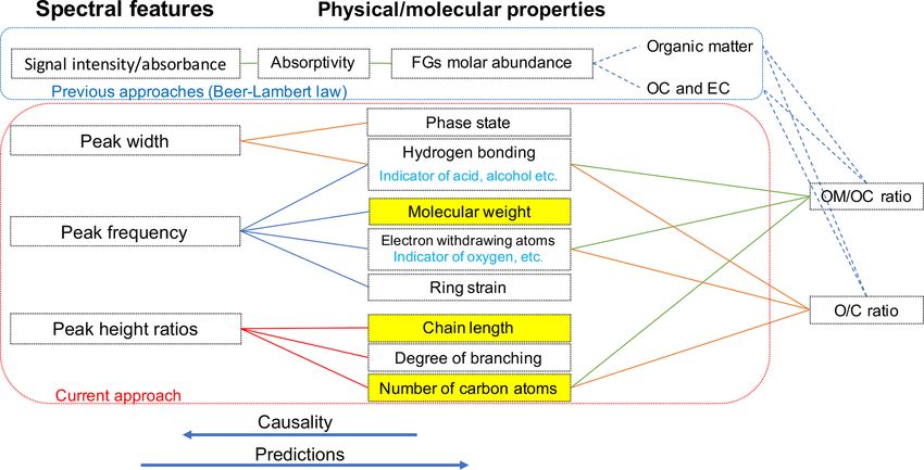
4808 A. Yazdani et al.: Mean carbon number and molecular weight in atmospheric aerosols
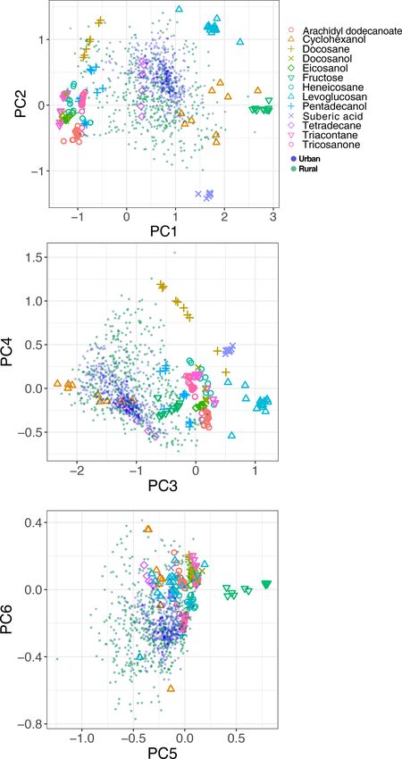
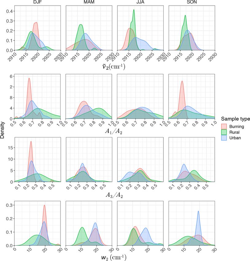
Figure 1. Normalized aliphatic C−H spectra of the laboratory standards (a) and several atmospheric samples (b). This figure shows variation
in absorbance profile among the standards and atmospheric samples.
able, while non-normalized absorbances were considered as especially aliphatic C−H, baseline correction could not be
independent variables (Takahama et al., 2013; Ruthenburg done properly in the aliphatic C−H region, resulting in irreg-
et al., 2014; Reggente et al., 2016). In this manner, linear ular and negative absorbance profiles. These samples were
models resembling the Bouguer–Lambert–Beer law were de- omitted from further analysis and only 798 were analyzed in
veloped. In this study, however, molecular weight and carbon this work. As can be seen from Fig. 4, data recovery is higher
number statistical models were developed using chemical at urban sites than at rural sites due to a usually more promi-
formulas of the laboratory standards (no molar abundance in- nent aliphatic C−H peak. Due to this undersampling, gener-
formation) and their normalized aliphatic C−H absorbances alizing the results of this work to the whole of rural samples
as independent variables. The current approach extracts de- should be done with caution.
tailed information from the mid-infrared spectrum comple-
mentary to previous approaches (Fig. 2). 2.2 Laboratory standards (sampling and analysis)
Compounds containing relevant functional groups to atmo-
2 Methods
spheric OM such as aliphatic C−H, alcohol and acid O−H,
We will describe the atmospheric samples as well as the lab- carbonyl C=O, and with different structures (straight chain
oratory standards for the calibration and test set in Sect. 2.1 and cyclic) and various chain lengths were used to produce
and 2.2. Thereafter, the methodology for data analysis and laboratory standards (Table 1). All compounds used for cre-
interpretation will be discussed in Sect. 2.3, 2.4, and 2.5. ating the standards contained aliphatic C−H, which is the
main focus of this study. Five of these compounds were
2.1 IMPROVE network monitoring sites (sampling alkanes, just containing aliphatic C−H. Three were straight-
and analysis) chain alcohols containing alcohol O−H as well. One was
cyclic alcohol, and one was a cyclic ketone having carbonyl
Particulate matter with diameter less than 2.5 µm (PM2.5 ) C=O; two were cyclic (not aromatic) sugar derivatives con-
was collected on PTFE filters (25 mm diameter Teflo® mem- taining several O−H groups. The calibration set also con-
brane, Pall Corporation) every third day for 24 h, midnight tained an ester, a ketone, and one dicarboxylic acid. In ad-
to midnight, at a nominal flow rate of 22.8 L min−1 during dition to relevance to atmospheric OM, these standards were
2011 and 2013 at selected sites in the IMPROVE network selected based on the availability of spectroscopic data and
(http://vista.cira.colostate.edu/improve/, last access: 8 Octo- their suitability for atomization. These compounds had com-
ber 2020). There are, in total, 814 samples collected at 7 sites parable absorption coefficients for aliphatic C−H, and the ef-
in the US in the year 2011 and 2161 samples collected at 16 fect of other functional groups, heteroatoms, and the molec-
different sites in the US 2013 (see Fig. 3). Overall, 1 out 7 ular structure was analyzed indirectly via the change in the
sites in 2011 and 4 out of 16 of sites in 2013 are urban sites, aliphatic C−H absorbance profile. Some of the laboratory
and the rest are rural. FT-IR analysis was performed on the standards and their resulting spectra were taken from Ruthen-
PTFE filters using a Bruker Tensor 27 FT-IR spectrometer burg et al. (2014). The rest were created (using a similar
equipped with a liquid nitrogen-cooled, wideband mercury– protocol) from methanolic solutions with a concentration
cadmium–telluride (MCT) detector and at a resolution of of 0.1 g L−1 and analyzed by FT-IR as follows. Atomized
4 cm−1 (data intervals of 1.93 cm−1 ; Nyquist sampling). For aerosols of the desired compounds were first generated by
samples with low molar abundance of organic compounds, a TSI Model 3076 aerosol generator using the methanolic
Atmos. Meas. Tech., 14, 4805–4827, 2021 https://doi.org/10.5194/amt-14-4805-2021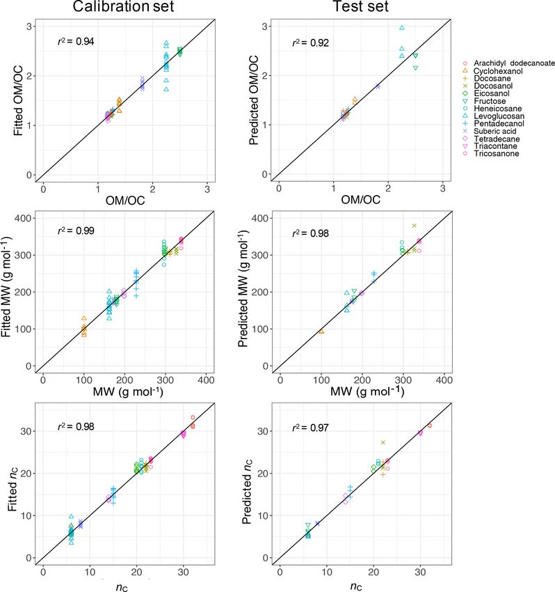
A. Yazdani et al.: Mean carbon number and molecular weight in atmospheric aerosols                                                  4809

Figure 2. Diagram showing the relation between spectral features and molecular or physical properties. The way previous approaches (e.g.,
Ruthenburg et al., 2014; Takahama et al., 2013) and the current approach use the mid-infrared spectrum to estimate different parameters is
shown in blue and red boxes, respectively. Highlighted molecular properties can only be estimated using the current approach.

Figure 3. The location of IMPROVE sites used for this work (the        Figure 4. Percentage of the samples which were recovered from
US and Alaska); the year in which samples are taken is differenti-     each category (sample type and season) after baseline correction.
ated by color and the type of the site by point shape.                 The number of samples in each category is shown in red.

                                                                       (DLaTGS) detector, with the same spectral resolution as the
solutions. Then, these particles were conducted by the flow            spectra of the ambient samples.
system towards a 47 mm PTFE filter (Teflo® membrane, Pall                 In total, 168 laboratory samples with different composition
Corporation), where they were collected. The flow system               and molar abundance (absorption amplitude ranging from
was composed of a silica gel dryer (for drying the aerosols            0.001 to 2 before normalization) were used, from which a
before collection), a sharp-cut-off 1 µm cyclone, and a diluter        subset of 43 samples was kept as a test set and the rest were
system (which facilitated the adjustment of aerosol concen-            used as the calibration set. The test set was used solely for
tration in the line). The pressure drop needed for the flow            the purpose of evaluation of the statistical models developed
through the filter was provided by a rotary vacuum pump                using the calibration set. However, the final statistical mod-
(Gast 0523-101Q-G588NDX), and the filter flow was con-                 els, which were applied to ambient samples, were developed
trolled by a gas-flow controller (Alicat MCR-100-SLPM-                 using all 168 laboratory standards to increase the precision.
D/5M). The mass on the filters ranged from few micrograms
to tens of micrograms. After collecting the aerosols on the            2.3   Baseline correction and normalization
filters, FT-IR analysis was performed on the PTFE filters us-
ing a Bruker Vertex 80 FT-IR spectrometer equipped with                The baseline removal is often a useful step in mid-infrared
a deuterated lanthanum α alanine doped triglycine sulfate              spectroscopy on PTFE filters, like in other methods of spec-

https://doi.org/10.5194/amt-14-4805-2021                                                  Atmos. Meas. Tech., 14, 4805–4827, 2021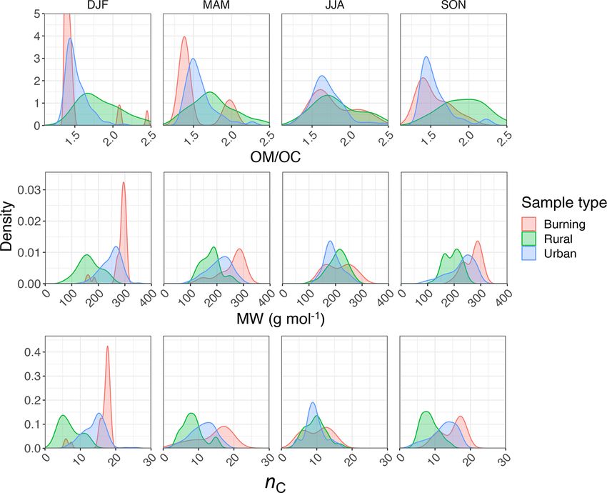
4810                                 A. Yazdani et al.: Mean carbon number and molecular weight in atmospheric aerosols

Table 1. Chemicals used in the calibration set to analyze the effect of different physical or chemical properties of organic molecules on
aliphatic C−H absorbance profile.

                                                                                       Phase       Molecular
                                                                                       state          weight
                 Compound name            Formula       Class                          at 25 ◦ C   (g mol−1 )   OM/OC
                 Tetradecane              C14 H30       alkane                         liquid          198.4       1.18
                 Hexadecane               C16 H34       alkane                         liquid          226.4       1.18
                 Heneicosane              C21 H44       alkane                         solid           296.6       1.18
                 Docosane                 C22 H46       alkane                         solid           310.6       1.18
                 Triacontane              C30 H62       alkane                         solid           422.8       1.17
                 1-Pentadecanol           C15 H32 O     alkanol                        solid           228.4       1.27
                 1-Eicosanol              C20 H42 O     alkanol                        solid           298.6       1.24
                 1-Docosanol              C22 H46 O     alkanol                        solid           326.6       1.24
                 Cyclohexanol             C6 H12 O      cyclic alcohol                 liquid          100.2       1.39
                 Cyclohexanone            C6 H10 O      cyclic ketone                  liquid           98.1       1.36
                 Fructose                 C6 H12 O6     sugars and their derivatives   solid           180.2       2.50
                 Levoglucosan             C6 H12 O5     sugars and their derivatives   solid           162.1       2.25
                 Suberic acid             C8 H14 O4     dicarboxylic acid              solid           174.2       1.81
                 Arachidyl dodecanoate    C32 H64 O2    ester                          solid           480.9       1.25
                 12-Tricosanone           C23 H46 O     ketone                         solid           338.7       1.23

troscopy. The baseline arises from light scattering by the fil-        e is a vector of residuals (y and X are assumed to be cen-
ter membrane (Mcclenny et al., 1985) and particles collected           tered). In spectroscopic applications, due to indeterminacy
on the filter as well as electronic transitions of some car-           (more independent variables than the number of samples)
bonaceous materials (Russo et al., 2014; Parks et al., 2019).          and collinearity (inter-correlation between independent vari-
For baseline removal, we used the smoothing spline method              able), the ordinary least squares (OLS) method is not appli-
on the 1500–4000 cm−1 region, where PTFE filter does not               cable or is not robust unless regularized. Among the com-
absorb, with parameter selection criteria similar to the ap-           mon methods developed for treating such a data structure, we
proach taken by Kuzmiakova et al. (2016). Briefly, a cubic             chose univariate (y is a vector, i.e., has one variable) partial
smoothing spline was fitted to the spectrum and then was               least squares regression (PLSR) for this work (Wold et al.,
subtracted from the raw spectrum to obtain the pure con-               1983). Univariate PLSR projects X onto P basis with orthog-
tribution of functional groups at each wavelength. The an-             onal scores T and residual matrix E (Eq. 3) such that the
alyte region (the aliphatic C−H absorption region; 2800–               covariance between each score column and y is maximized
3000 cm−1 ) was manually excluded from the baseline by set-            (in each step of deflation). Thereafter, the response variable
ting the weights in this region to zero in the smoothing spline        y is regressed linearly against the scores (Eq. 4). In Eq. (4),
objective function (refer to Kuzmiakova et al., 2016). The             c is the regression coefficient of y as a function of scores (T)
rest of the spectrum between 1500 and 4000 cm−1 was in-                and f is the vector of residuals.
cluded in the baseline by setting the weights to 1. After base-
line correction, the aliphatic C−H absorbances were scaled             X = TP> + E                                                   (3)
between 0 and 1 (Fig. 1) for all spectra so that the absorbance        y = Tc + f                                                    (4)
profiles were comparable regardless of the absorbance inten-
sity (functional group abundance).                                        Determining the optimum number of latent variables
                                                                       (LVs), which are linear combinations of original wavenum-
2.4    Building the calibration models                                 bers in this study, is an essential step for developing cali-
                                                                       bration models with predictive capability. After solving the
In order to estimate molecular weight and carbon number                PLSR problem for calibration models with different num-
from the normalized aliphatic C−H absorbances in the mid-              ber of LVs, we ran a repeated 10-fold cross validation on
infrared spectra, we seek the solution of the following linear         the calibration models and calculated the root mean square
equation for the calibration models:                                   error (RMSE) of predictions (for the calibration set) for
                                                                       each model. Thereafter, the model whose RMSE was within
y = Xb + e,                                                     (2)
                                                                       1 standard error from the calibration model with minimum
where X is the normalized spectra matrix (the aliphatic C−H            RMSE and had fewer LVs (i.e., a simpler model) was chosen
absorption region, 2800–3000 cm−1 ), y is the vector of re-            (Hastie et al., 2009). Based on the above-mentioned proce-
sponse variable (molecular weight or carbon number), and               dure, the optimal number of LVs for molecular weight and

Atmos. Meas. Tech., 14, 4805–4827, 2021                                                  https://doi.org/10.5194/amt-14-4805-2021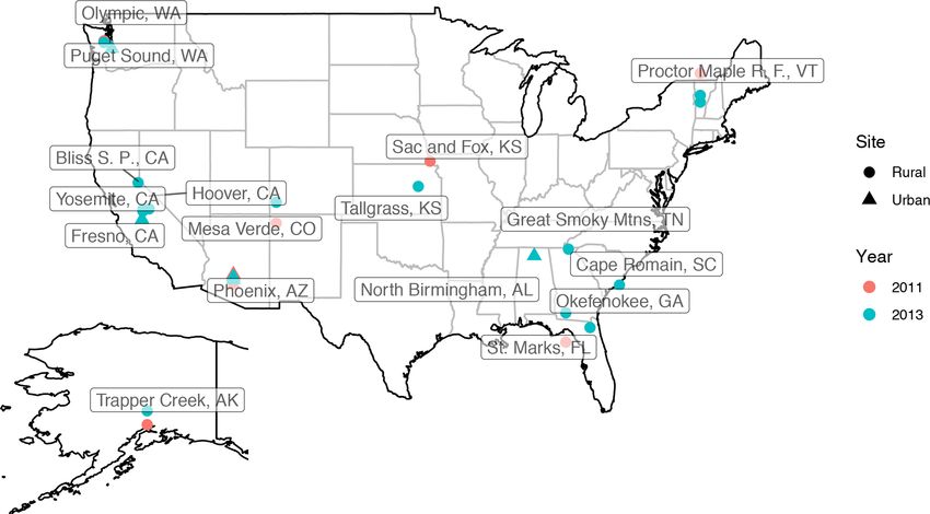
A. Yazdani et al.: Mean carbon number and molecular weight in atmospheric aerosols                                           4811

carbon number calibration models was found to be 19 and
20, respectively.

2.5    Interpreting the calibration models using the basic
       spectral features

Although the PLSR models have considerably fewer LVs
(approximately 20) than the original wavenumbers (105), the
lack of physical interpretability and remaining number of
LVs still hinders their physical interpretation. Therefore, we
first analyze the basic (physically interpretable) features of
the mid-infrared spectrum – peak frequencies, widths, and
ratios in the aliphatic C−H region – for the calibration set
and their relation with carbon number and molecular weight
(Sect. 3.1). Spatial and temporal variations of these patterns
in the atmospheric samples are also analyzed and related to
similar patterns in the laboratory standards.
   The four basic features of the ambient sample spectra were     Figure 5. A sample C−H spectrum showing the convention of
used to build a classification and regression tree (CART)         peak parameters used in this study. The symmetric CH2 (ν̃s CH2 )
                                                                  wavenumber is denoted by ν̃1 . The asymmetric CH2 (ν̃as CH2 )
(Breiman et al., 1983) to approximate the PLSR predictions
                                                                  wavenumber is denoted by ν̃2 and the asymmetric CH3 (ν̃as CH3 )
of mean molecular weight and carbon number and to bet-            wavenumber by ν̃3 . Absorbance and width of the ith peak are also
ter understand their connection with the underlying spec-         denoted by Ai and wi , respectively.
tral absorption characteristics. In this approach, binary deci-
sion trees are generated to classify the PLSR estimates based
on partitioned domains of their basic spectral features. The         Figure 5 shows the convention of spectral features in the
CART algorithm expands the trees in the order of decreas-         aliphatic C−H (2800–3000 cm−1 ) region used in this study.
ing explanatory power until certain stopping conditions (e.g.,    Apart from methine group (tertiary C−H), which has a very
minimum number of observations in terminal nodes or mini-         weak absorption (Pavia et al., 2008), there are two doublets
mum improvement of explanatory power at each step of split-       in this region corresponding to CH2 and CH3 symmetric
ting) are satisfied.                                              and asymmetric stretching vibrations. The CH3 symmetric
                                                                  peak is typically suppressed by the surrounding peaks and is
3     Results and discussion                                      not completely distinguishable. Among the remaining peaks,
                                                                  the symmetric CH2 (ν̃s CH2 ) wavenumber is denoted by ν̃1 .
First, the basic features of the aliphatic C−H profile are dis-   Likewise, the asymmetric CH2 (ν̃as CH2 ) wavenumber is de-
cussed in the atmospheric and the laboratory samples, fol-        noted by ν̃2 and the asymmetric CH3 (ν̃as CH3 ) wavenumber
lowed by a similarity check between the two (Sect. 3.1).          by ν̃3 . Absorbance and peak width of the ith peak are also
Then, development of calibration models for predicting            denoted by Ai and wi , respectively.
molecular weight and carbon is described, followed by in-            In the next subsections, the variations of the mentioned
vestigation of their performance in the calibration and test      spectral features are studied in the laboratory standards and
(Sect. 3.2). Thereafter, the model estimates are discussed for    atmospheric samples. For this purpose, the atmospheric sam-
atmospheric samples and compared to the results reported in       ples are separated into urban, rural, and burning categories.
literature (Sect. 3.3). Finally, the basic features introduced    The burning category constitutes 95 samples of urban or ru-
earlier are used to classify the results of the sophisticated     ral sites and is taken from clusters 9a, 9b, and 10 of Bürki
(PLSR) models in order to obtain a better understanding of        et al. (2020) based on their spectral similarity. These samples
the way they function (Sect. 3.4).                                are believed to be influenced by residential wood burning or
                                                                  wildfires since they were usually collected during a known
3.1    Basic features                                             fire period (Rim Fire in California in 2013) or in Phoenix,
                                                                  AZ, during winter months when residential wood burning
Basic features of the spectrum in the aliphatic C−H region        typically occurs (Pope et al., 2017).
were calculated for atmospheric samples and laboratory stan-
dards to study their temporal and spatial variation and their     3.1.1   Asymmetric CH2 peak wavenumber (ν̃2 )
relation with molecular properties such as molecular weight,
carbon number, and the OM/OC ratio. These variables, al-          We calculated the second peak wavenumber (ν̃2 ) for the lab-
though few, can give a good estimate of the absorbance pro-       oratory standards and atmospheric samples using a simple
file and make it more interpretable.                              peak-finding algorithm based on the first and second numeri-

https://doi.org/10.5194/amt-14-4805-2021                                            Atmos. Meas. Tech., 14, 4805–4827, 2021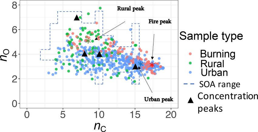
4812                                 A. Yazdani et al.: Mean carbon number and molecular weight in atmospheric aerosols

                                                                     strong dimerization. As mentioned in Sect. 1.2, the A1 /A2
                                                                     ratio compares symmetric and asymmetric absorbance of
                                                                     methylene, and its connection with carbon number has al-
                                                                     ready been highlighted in FT-IR analysis of some types of
                                                                     diesel fuels (Price et al., 2017). Increase in A1 /A2 is also ob-
                                                                     served between solid and liquids, consistent with the work
                                                                     of Corsetti et al. (2017). We also observe a nonlinear rela-
                                                                     tion between the A3 /A2 ratio and carbon number with differ-
                                                                     ent levels based on branching and terminal functionalization
                                                                     (Fig. 8b). This ratio is equal to zero for molecules lacking
                                                                     methyl group such as simple cyclic molecules while increas-
                                                                     ing as the number of branches containing terminal methyl
                                                                     increases.
Figure 6. Scatter plot showing the variation of the second peak
wavenumber (ν̃2 ) with molecular weight (MW) in the calibration         Results show a clear separation in atmospheric samples
set, affected by the OM/OC ratio and phase state. The black line     regarding the sample type and season for both A1 /A2 and
shows the theoretical frequency with a spring constant equal to      A3 /A2 ratios (Fig. 7, second and third row). The samples
103 N m−1 for all C−H bonds. The OM/OC ratio and phase state         influenced by burning usually have the lowest A1 /A2 ratio
are shown for the samples. The error bars show uncertainty in cal-   (Fig. 7, second row). This observation is consistent with the
culated peak frequency due to FT-IR scan resolution.                 presence of molecules with longer chains, as observed for
                                                                     laboratory samples. Bürki et al. (2020) showed that the ur-
                                                                     ban samples (in the same dataset) have their highest aver-
cal derivatives of the spectrum. For the laboratory standards,       age OM/OC ratio in summer which is concurrent with their
the frequency generally decreases with increasing molecular          highest A1 /A2 ratio, which suggests shorter chain length.
weight until it reaches an asymptotic state after 200 g mol−1        The highest A1 /A2 ratio for rural samples is observed in
(Fig. 6). The curve in Fig. 6 shows the theoretical peak fre-        spring when the aerosols are highly oxidized (Bürki et al.,
quency of the aliphatic C−H when the bond spring con-                2020). This suggests that aged aerosols have lower carbon
stant is assumed to be 103 N m−1 (Pavia et al., 2008), and           number probably due to the fragmentation process. The mea-
the reduced mass is calculated based on a ball-and-string as-        sured A1 /A2 ratio for the majority of the atmospheric sam-
sumption composed of the hydrogen atom (first “ball”) and            ples ranges between 0.6 and 0.8, which is consistent with
the rest of molecule (second “ball”). The only effect consid-        the value for laboratory standards. Results also show that
ered in this model is the variation of the reduced mass of           the A3 /A2 ratio is higher in rural samples compared to ur-
the oscillator. The fact that the less-oxygenated laboratory         ban samples (with the exception of spring), suggesting a
samples follow the theoretical line closely implies that the         higher CH3 to CH2 abundance in those samples. This ob-
value of the spring constant considered here is, on average,         servation can be due to lower carbon number or higher num-
a good approximation. However, especially for highly oxy-            ber branches containing CH3 . Like the A1 /A2 ratio, we ob-
genated (high OM/OC ratio) molecules and those with in               serve fewer samples with low A3 /A2 ratios at urban sites
liquid phase (which have a lower molecular weight), the ab-          in summertime. The A3 /A2 ratio falls between 0.1 and 0.4
sorption frequency deviates from the theoretical line (higher        for the majority of the atmospheric samples, which is consis-
frequency) due to higher levels of intermolecular interaction.       tent with the value for laboratory standards. It is worth not-
   Regarding the atmospheric samples, most of categories             ing that peaks in atmospheric samples are more overlapped
have a peak density in 2915–2925 cm−1 , close to that of             than laboratory standards, which makes calculation of peak
straight-chain molecules of the laboratory standards (Fig. 7,        ratios based on extrema of the original spectra imprecise. As
first row). Urban samples have a wider shoulder on the right         a result, a peak-fitting method based on Gaussian peaks was
side (around 2925 cm−1 ) in summer when the samples are              applied to atmospheric samples in order to obtain the peak
expected to be more aged. Other variations are believed to           ratios more precisely.
be insignificant considering the scan resolution of the FT-IR
instrument.                                                          3.1.3   Peak width (wi )

3.1.2   Peak height ratios (Ai /A2 )                                 We observe a clear correlation between w2 and the OM/OC
                                                                     ratio in the calibration set when solid and liquid phases are
Analyzing the laboratory standards shows that a relatively           considered separately (Fig. 9). As mentioned in Sect. 1.2, hy-
linear but scattered relation exists between carbon number           drogen bonding increases the peak width, and the extent of
and the A1 /A2 ratio in the calibration set (Fig. 8a). Suberic       hydrogen bonding is usually a good indicator of the OM/OC
acid, which is the only dicarboxylic acid in the laboratory          ratio. This is because hydroxyl, hydroperoxyl, and carboxyl
standards, does not follow the general trend, probably due to        groups, which form hydrogen bonds, are among the most ef-

Atmos. Meas. Tech., 14, 4805–4827, 2021                                               https://doi.org/10.5194/amt-14-4805-2021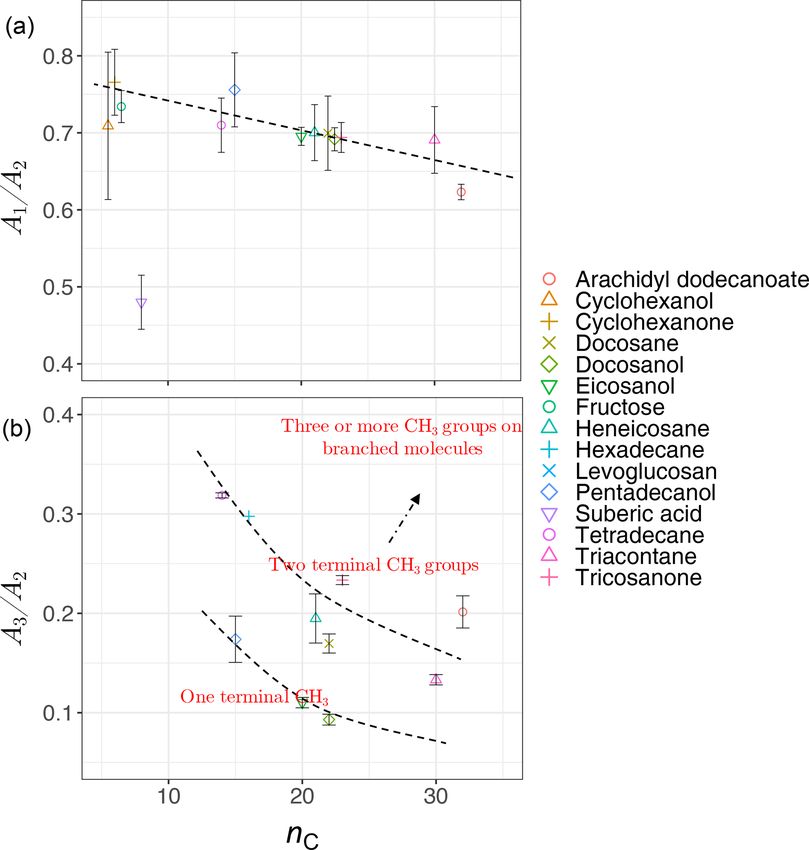
A. Yazdani et al.: Mean carbon number and molecular weight in atmospheric aerosols                                                   4813

Figure 7. Kernel density estimate of second peak wavenumber (ν̃2 ), the ratio of peak heights of symmetric CH2 to asymmetric CH2 stretching
(A1 /A2 ), the ratio of peak heights of asymmetric CH3 to asymmetric CH2 stretching (A3 /A2 ), and the second peak width (w2 ) of the
aliphatic C−H band in the mid-infrared spectra of the atmospheric samples segregated based on sample type and season.

fective functional groups in secondary organic aerosol (SOA)            ple category. Rural samples have a smaller value of w2 com-
formation due to the significant vapor pressure reduction they          pared to urban and burning samples, although the former are
cause (Seinfeld and Pandis, 2016). In this study, w2 is defined         usually more oxidized (have higher OM/OC ratio). This ob-
as the peak width at 75 % of the maximum amplitude. This                servation suggests that other factors such as phase state and
position is chosen for robustness of the measurement algo-              statistical effects likely outweigh the oxygenation effect on
rithm (to avoid interference with other peaks); however, it             absorption peak width.
can be converted to full width at half maximum (FWHM) as-
suming the proper peak profile (w2 is 65 % of FWHM for a                3.1.4   Spectral similarity (dimension reduction)
Gaussian peak). In addition to hydrogen bonding and phase
state, superposition of a multitude of peaks with slightly dif-         In previous sections, the basic features of spectra in the
ferent profiles can also have a statistical positive or negative        aliphatic C−H region were presented and discussed for the
effect on the peak width in mixtures (see Sect. S1 in the               atmospheric samples and laboratory standards. Here, we
Supplement). The observed peak width in the mid-infrared                check the spectral similarity between atmospheric complex
spectra of the atmospheric samples is the result of all above-          mixtures and laboratory pure standards by means of princi-
mentioned factors. However, since all laboratory standards              pal component analysis (PCA), before developing calibration
are produced with pure compounds, the significance of the               models.
mixture effect cannot be evaluated.                                        The spectral data of laboratory standards are highly
   Figure 7 (fourth row) shows a distinct distribution of w2            collinear as can be seen from their correlation matrix heat
considering spatial and temporal variations as well as sam-             map (Fig. A1). In this case, PCA is efficient for reducing the
                                                                        data dimension such that only the first six principal compo-

https://doi.org/10.5194/amt-14-4805-2021                                                   Atmos. Meas. Tech., 14, 4805–4827, 2021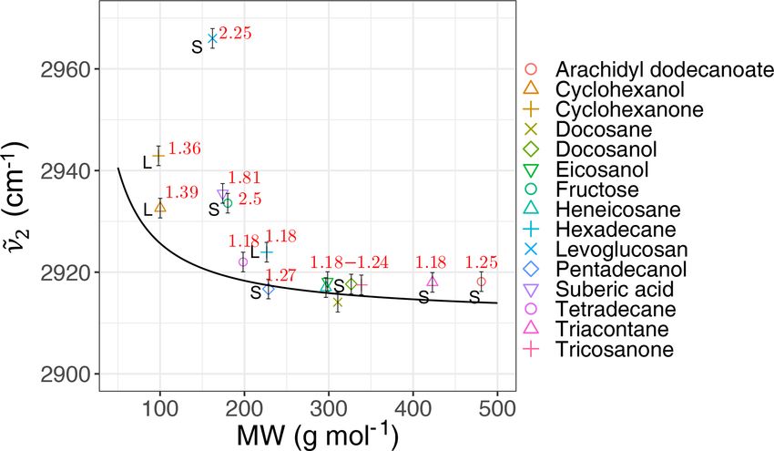
4814                                  A. Yazdani et al.: Mean carbon number and molecular weight in atmospheric aerosols

Figure 8. Scatter plots showing the relation between carbon num-
ber (nC ) and the ratio of peak heights of symmetric CH2 to asym-
metric CH2 stretching (A1 /A2 , a), and the ratio of peak heights of
asymmetric CH3 stretching to asymmetric CH2 stretching (A3 /A2 ,
b), averaged for each substance in laboratory standards. Error bars
show ± 1 standard error from the average, and dashed lines are vi-
sual guides for the trends and levels.

                                                                       Figure 10. Bi-plots showing the scores of normalized spectra of
                                                                       laboratory standards (color) and normalized spectra of atmospheric
                                                                       samples (filled circles) projected onto the first six principal compo-
                                                                       nents calculated for laboratory standards and listed in Table 2.

Figure 9. The average value of second peak width (w2 ) measured        ticularly urban ones, are clustered close to tetradecane for
for each compound in the calibration set versus the OM/OC ra-
                                                                       the first four PCs (Fig. 10); greater differentiation is found
tio, colored based on compound phase state at laboratory condition
(25 ◦ C). Error bars show ± 1 standard error from the average, and
                                                                       among the higher PCs. This observation suggests that the
dashed lines are visual guides.                                        laboratory standards are able to capture the main variations
                                                                       in the spectra of atmospheric samples, which have a more
                                                                       regular aliphatic C−H profile close to that of straight-chain
nents (PCs) explain around 99 % of variance in the spectra             alkanes. We also found that PC3 appears to capture phase
(Table 2). For the sake of comparison, we have projected the           state information (see Sect. S2).
spectra of atmospheric samples onto the six PCs. The results
show that their scores, when projected onto laboratory PCs,
are surrounded by laboratory standards. Many spectra, par-

Atmos. Meas. Tech., 14, 4805–4827, 2021                                                   https://doi.org/10.5194/amt-14-4805-2021
A. Yazdani et al.: Mean carbon number and molecular weight in atmospheric aerosols 4815
Table 2. Importance of the first six principal components in the laboratory standards.
PC1 PC2 PC3 PC4 PC5 PC6
Standard deviation 1.414 0.668 0.647 0.332 0.203 0.133
Proportion of variance 0.651 0.145 0.136 0.036 0.014 0.006
Cumulative proportion 0.651 0.796 0.932 0.968 0.982 0.988
3.2 Developing and evaluating the calibration models Thus, the absorption coefficient of aliphatic C−H has been
assumed to be relatively similar between the compounds ex-
PLSR with cross validation was used to develop quantita- isting in atmospheric samples. Although the aliphatic C−H
tive models for molecular weight (MW) and carbon number absorption coefficients of the laboratory standards were sim-
(nC ) with the calibration set composed of 143 samples in- ilar in this study, the variability of this absorption coefficient
cluding all compounds over the available mass range. The is relatively less studied for compounds existing in the at-
OM/OC ratio was then calculated from these two parame- mospheric OM and needs to be addressed in the future. This
MW assumption is a potential source of error that may change
ters (OM/OC = 12.01n C
). The developed PLSR models gave
reasonably good fit results (r 2 ranging from 0.94 to 0.99) for the accuracy of the results, but the estimates for atmospheric
molecular weight, carbon number, and indirect OM/OC ratio samples shown in the following sections suggest that this as-
in the calibration set (Fig. 11). sumption does not overwhelm the findings.
The prediction ability of the PLSR models was then evalu-
ated using a test set composed of 43 samples which were not 3.3.1 OM/OC ratio
used for developing the models. The PLSR models also per-
formed reasonably well in predicting molecular weight, car- The OM/OC ratio is the first parameter that we investigate
bon number, and OM/OC ratio in the test set with r 2 rang- here since it has been studied extensively in atmospheric
ing from 0.92 to 0.98 (Fig. 11). The predictions with high aerosols (Bürki et al., 2020; Hand et al., 2019; Ruthenburg
relative error were attributed to laboratory samples with low et al., 2014; Takahama et al., 2011; Simon et al., 2011; Aiken
molar abundance (low signal-to-noise ratio), for which the et al., 2008). Moreover, it can be used as an indirect evalua-
baseline correction had the highest uncertainty. This is not tion for mean molecular weight and mean carbon number es-
a concern when applying the PLSR models to atmospheric timates as the indirect OM/OC ratio is calculated from those
samples since the atmospheric samples with low signal-to- two. An indirect OM/OC estimate that is consistent with pre-
noise ratio were omitted in the first step (Sect. 2.1). vious studies implies that estimates of molecular weight to
carbon number are also likely to be reasonable.
3.3 Applying the calibration models to atmospheric The OM/OC ratio is estimated to be generally lower for
samples urban samples (≈ 1.5) than rural samples (≈ 1.8; Fig. 14,
first row). The lower OM/OC ratio at urban sites is thought
After checking the performance of the PLSR models on the to be related to emission sources that are generally hydro-
calibration and test set, all laboratory standards were used carbon, with low OM/OC ratio emitted from gasoline and
to build calibration models that were applied to the ambient diesel vehicles (fuel combustion and unburned motor oil)
samples. In the following sections, the estimates of OM/OC, as a major part of anthropogenic SOA precursors (Gentner
mean molecular weight, and mean carbon number for the et al., 2012), as well as cooking. These organic molecules
ambient samples are shown in different categories based on do not undergo significant oxidation and aging as the mon-
season and sample type (rural, urban, and burning) after itoring sites are generally close to the emission sources. In
omitting the physically unreasonable values. Thereafter, the contrast, organic aerosols usually undergo several steps of
trends and absolute values are compared to previous studies oxidation and receive substantial condensation of oxidized
(when available) and our expectations based on aging pro- vapors, which results in higher OM/OC ratio at rural and
cess and aerosol emission sources. remote sites. Previous studies using several different meth-
In this work, we have assumed that we can obtain mean ods (including FT-IR and AMS) show the same trend at ur-
mixture (atmospheric samples) properties from the normal- ban and rural sites (Ruthenburg et al., 2014; Zhang et al.,
ized spectrum of a mixture using the calibration models de- 2007; Simon et al., 2011; Bürki et al., 2020). In addition, the
veloped for pure compounds (laboratory standards). This as- majority of the samples are in the range that is usually con-
sumption relies on the linearity of the property estimation sidered for OM/OC ratio, i.e., 1.4–1.7 (Russell, 2003). We
models (which is consistent with our calibrations; Eq. 4) and also observe that samples influenced by burning, especially
equality of the absorption coefficients of the compounds ex- residential wood burning, have lower OM/OC ratio (≈ 1.4)
isting in the mixture (see Appendix B for more information). than those associated with more oxidized aerosol such as ru-
https://doi.org/10.5194/amt-14-4805-2021 Atmos. Meas. Tech., 14, 4805–4827, 20214816 A. Yazdani et al.: Mean carbon number and molecular weight in atmospheric aerosols
Figure 11. Scatter plot of fitted (predicted) indirect OM/OC ratio, MW, and nC against the values from chemical formula of the calibration
set (test set). The diagonal black lines indicate the perfect fit (1 : 1).
ral sites, consistent with OM/OC estimates of Bürki et al. to 100 %, and compared our indirect OM/OC ratio esti-
(2020). mates to the corresponding ones calculated by Bürki et al.
The OM/OC ratio at urban sites is estimated to be higher (2020). The latter method uses molar abundance information
in summer compared to other seasons, especially winter of functional groups in laboratory standards in addition to a
(Fig. 14, first row) which is believed to be caused by more much wider region of non-normalized mid-infrared spectrum
intense photochemical aging in summertime (Kroll and Se- (1500–4000 cm−1 ). The median seasonal OM/OC ratios of
infeld, 2008). At rural sites, the trend becomes more compli- this study underpredict that of Bürki et al. (2020) by 0.12 on
cated, as vegetation, a major biogenic SOA emission source, average, while reproducing the same temporal trends. Some
is more active in summertime (Yuan et al., 2018; Seinfeld and of the discrepancies may be due to insensitivity of spectral
Pandis, 2016). Samples influenced by burning are also esti- features to molecular characteristics in certain domains – for
mated to have higher OM/OC in summer when samples are instance, the variation of peak frequency ν̃2 diminishes with
affected by wildfires compared to winter when burning sam- increasing molecular weight (Sect. 3.1.1). However, the over-
ples are mostly affected by residential wood burning. How- all agreement between the two methods is reasonable consid-
ever, the contribution of photooxidation relative to emission ering the indirect nature of estimates in our work (Fig. 12).
sources is not clear in this case, as they are coupled in these
observations (Bürki et al., 2020). 3.3.2 Molecular weight
In order to have a direct comparison with other methods,
we chose the Phoenix, AZ, monitoring site, for which re- The PLSR model estimates the mean molecular weight to
covery percentage of the baseline correction method is close range between 100 and 350 g mol−1 for the majority of the
samples (Fig. 14, second row). To the best of the authors’
Atmos. Meas. Tech., 14, 4805–4827, 2021 https://doi.org/10.5194/amt-14-4805-2021A. Yazdani et al.: Mean carbon number and molecular weight in atmospheric aerosols 4817
tation during more intense photooxidation in summer (Hand
et al., 2019; Jimenez et al., 2009) for emission sources that
do not change drastically between the two seasons. The same
phenomenon is observed in LDI mass spectra of some urban
samples in summer and winter reported by Kalberer et al.
(2006). Although the reduction in mean molecular weight
due to fragmentation can be compensated for by addition of
heavy atoms to the molecule during oxidation, our results
suggest that the overall direction of photooxidation at urban
sites is reduction of the mean molecular weight.
3.3.3 Carbon number
The PLSR carbon number model estimates that the recov-
Figure 12. Bar chart showing median OM/OC ratio calculated for ered rural samples usually have lower mean carbon number
each season based on samples collected at the Phoenix, AZ, moni- compared to urban samples and the samples influenced by
toring site using our method and the one used by Bürki et al. (2020). burning (Fig. 14, third row). Higher mean carbon number
estimates at urban sites (highest probability density around
16), which are coincident with high elemental carbon (EC)
knowledge, no extensive study has been performed on mean values from TOR measurements (Fig. C1), can be attributed
molecular weight of ambient organic aerosol constituents. to major EC sources such as combustion of fossil fuel and
Nevertheless, the estimated range is reasonably close to that biomass. This is also consistent with high SOA formation po-
of the studies that have been done. Those studies measured tential of molecules with 15–25 carbon in diesel fuel shown
molecular weights up to 200 g mol−1 for SOA constituents by Gentner et al. (2012). Samples affected by burning are es-
using GC/MS and ion chromatography (Cocker III et al., timated to have the highest mean carbon number among all
2001; Jang and Kamens, 2001b; Kalberer, 2004), an av- samples. This observation is consistent with the emissions of
erage molecular weight between 200 and 300 g mol−1 for plant cuticle waxes, mainly composed of straight-chain hy-
atmospheric humic-like substances (HULIS) using electro- drocarbons, observed during biomass burning (Hawkins and
spray ionization (ESI) (Graber and Rudich, 2006), and an Russell, 2010) as well as HULIS (Graber and Rudich, 2006).
average molecular weight between 300 and 450 g mol−1 We also observe a decrease in estimated mean carbon number
for oligomers formed in a smog chamber, measured us- of urban samples from winter to summer, suggesting frag-
ing laser desorption/ionization mass spectrometry (LDI-MS) mentation during aging and photooxidation processes.
(Kalberer et al., 2006). Although particle-phase oligomer- The carbon–oxygen estimates of the PLSR models are
ization processes result in high-MW compounds (Jang and consistent with the existing numerical simulation. We com-
Kamens, 2001a; Tolocka et al., 2004; Shiraiwa et al., 2014), pared our estimates with the numerical simulations by Jathar
the abundance of these compounds is usually debated since et al. (2015). A multi-generational oxidation model used by
the available experimental results regarding the reversibility Jathar et al. (2015) (Statistical Oxidation Model, SOM, in a
of accretion reactions are contradictory (Kroll and Seinfeld, 3-D air quality model) for simulating SOA in Los Angeles
2008). Moreover, oligomer formation may be overestimated and Atlanta (two urban locations) shows that carbon num-
in laboratory conditions compared to atmospheric particles ber in SOA ranges from 3 to 15 with the concentration peaks
(Kroll and Seinfeld, 2008; Kalberer, 2004; Trump and Don- around 7, 10, and 15 (Fig. 13). For this comparison, we calcu-
ahue, 2014). lated the carbon–oxygen grid from our molecular weight and
The PLSR molecular weight model estimates a lower carbon number estimates, assuming the organic molecules
mean molecular weight for rural samples (≈ 200 g mol−1 ) have a chemical formula of CNc H2Nc +2−No ONo (a common
compared to urban ones (≈ 240 g mol−1 ), while burning assumption and one used by Jathar et al., 2015). Our PLSR
samples are estimated to constitute the heaviest molecules (≈ models for the IMPROVE network estimate mean carbon
290 g mol−1 ). This observation is consistent with our knowl- number peaks (number density) for rural, urban, and burn-
edge of emission sources. Emissions in urban areas are influ- ing samples to be around 8, 16, and 18, respectively, while
enced by long-chain hydrocarbons from combustion prod- the total range is limited to 3–19 (Fig. 13). We also estimate
ucts and motor oil (Gentner et al., 2012), while biomass the oxygen number to range from 2 to 6 for the majority of
burning is accepted to be the primary source of high-MW the samples. It should be noted that this is an order of mag-
HULIS (Li et al., 2019). We also observe a decrease in mean nitude comparison since the time frame and the location of
molecular weight peak density in urban samples from win- the two studies are different and the numerical simulation by
ter to summer that is believed to be attributed to fragmen- Jathar et al. (2015) only considers SOA.
https://doi.org/10.5194/amt-14-4805-2021 Atmos. Meas. Tech., 14, 4805–4827, 20214818 A. Yazdani et al.: Mean carbon number and molecular weight in atmospheric aerosols
In summary, regression trees show that the predictions of
the PLSR models are generally consistent with the observed
trends of the basic features in the calibration set (Sect. S3
supports this conclusion for individual spectra for which the
PLSR models estimate quite different parameters). This ob-
servation implies that the PLSR predictions of carbon num-
ber and molecular weight are not independent of these basic
features. However, the sophisticated PLSR models use other
fine features in addition to the mentioned basic features to
extract more detailed information and to reduce variabilities
stemming from different sources such as baseline correction.
Figure 13. Comparison between the carbon–oxygen grid simulated
by Jathar et al. (2015) for Atlanta and Los Angeles with sample
points estimated for the IMPROVE network (2011 and 2013) from 4 Concluding remarks
the molecular weight and carbon number estimates of this study.
The dashed lines show the range of simulated carbon and oxygen, Normalized aliphatic C−H absorbances in the mid-infrared
and the triangles indicate the location of the highest SOA concen-
spectrum were used in this study to estimate carbon number
trations for the simulations of Jathar et al. (2015).
and molecular weight of the atmospheric OM. First, it was
shown that the spectral features, such as peak frequencies and
3.4 Calibration model interpretation ratios are correlated with carbon number, molecular weight,
and the OM/OC ratio for laboratory standards. We also ob-
Reducing the spectrum to four basic features introduced in served a meaningful temporal and spatial variation of those
Sect. 3.1 (ν̃2 , A3 /A2 , A1 /A2 , w2 ) is a manual data compres- features in atmospheric aerosol samples. Thereafter, PLSR
sion onto a basis set of interpretable variables. Though infor- models were developed on laboratory standards to estimate
mation loss is inevitable, it was shown in Sect. 3.1 that these the mentioned parameters in the atmospheric aerosol sam-
basic features are still sufficient for qualitative explanation of ples from the IMPROVE network. The estimated molecular
spectral variations associated with different emission source weight and carbon number reconstruct the OM/OC values
and aerosol aging process. In this section, predictions made in the atmospheric aerosols that are consistent with previous
by the PLSR models on the ambient samples are grouped studies with a reasonable difference (an average underpre-
based on the four basic features using CART (Fig. 15) in or- diction of 0.12). These new statistical models estimate lower
der to form a better understanding of how the sophisticated mean carbon number and mean molecular weight in more
PLSR models function. aged aerosols of the same source highlighting the fragmen-
The regression trees show that the peak ratios are observed tation role in aging process (Murphy et al., 2012). Moreover,
to be the main grouping parameter for both carbon number they estimate relatively less oxidized, heavier molecules with
and molecular weight (Fig. 15). The inverse relation of peak higher carbon number for samples influenced by burning.
ratios with carbon number appears in most of the splitting The findings show that the new technique can help us bet-
nodes of carbon number and molecular weight regression ter understand characteristics of OM due to source emissions
trees (Fig. 15). This is consistent with the observed relation and atmospheric processes. In addition, since carbon num-
between carbon number and peak ratios in the calibration set ber and molecular weight are important characteristics used
(Fig. 8). Assuming that molecular weight is highly correlated by recent conceptual models or parameterizations (e.g., Shi-
with carbon number, the classification of molecular weight raiwa et al., 2017a; Li et al., 2016; Pankow and Barsanti,
based on peak ratios is also expected. The peak frequency 2009; Kroll et al., 2011; Donahue et al., 2011) to describe
(ν̃2 ) appears once as a node in molecular weight tree and clas- evolution in OM composition, this technique can provide
sifies the estimates based on the same trend that was observed semi-quantitative, observational constraints on these varia-
in the calibration set (Fig. 6). The second peak width (w2 ) tions at the scale of the network as well as for laboratory
also appears few times in the nodes, probably adding infor- experiments. We also found that the phase state of the labo-
mation about the OM/OC ratio and phase state. The two trees ratory standards clearly affects their spectroscopic features.
shown in Fig. 15 explain only around 50 % of the variation These features can be used to develop predictive models that
of estimates made by the PLSR models. The explained vari- can estimate the phase state of atmospheric OM.
ation can be increased to an arbitrarily high number through Only around 27 % of the existing samples could be ana-
the use of more branches in the fitting dataset, but the predic- lyzed with our approach due baseline correction limitations
tive capability of regression trees for new samples depends posed by low OM mass (compared to inorganic mass) on the
highly on their similarity to the training set. filters. Undersampling is more severe at rural sites, although
expected trends (such as higher OM/OC ratio) are observed
even in the current subset. As a result, one should be cau-
Atmos. Meas. Tech., 14, 4805–4827, 2021 https://doi.org/10.5194/amt-14-4805-2021You can also read