Foraminiferal community response to seasonal anoxia in Lake Grevelingen (the Netherlands) - Biogeosciences
←
→
Page content transcription
If your browser does not render page correctly, please read the page content below
Biogeosciences, 17, 1415–1435, 2020
https://doi.org/10.5194/bg-17-1415-2020
© Author(s) 2020. This work is distributed under
the Creative Commons Attribution 4.0 License.

Foraminiferal community response to seasonal anoxia in
Lake Grevelingen (the Netherlands)
Julien Richirt1 , Bettina Riedel1,2 , Aurélia Mouret1 , Magali Schweizer1 , Dewi Langlet1,3 , Dorina Seitaj4 ,
Filip J. R. Meysman5,6 , Caroline P. Slomp7 , and Frans J. Jorissen1
1 UMR    6112 LPG-BIAF Recent and Fossil Bio-Indicators, University of Angers,
2 Boulevard Lavoisier, 49045 Angers, France
2 First Zoological Department, Vienna Museum of Natural History, Burgring 7, 1010 Vienna, Austria
3 Univ. Lille, CNRS, Univ. Littoral Côte d’Opale, UMR8187, LOG, Laboratoire d’Océanologie et

de Géosciences, 62930 Wimereux, France
4 Department of Ecosystem Studies, Royal Netherlands Institute for Sea Research (NIOZ), Yerseke, the Netherlands
5 Department of Biology, University of Antwerp, Universiteitsplein 1, 2610 Wilrijk, Belgium
6 Department of Biotechnology, Delft University of Technology, 2629 HZ Delft, the Netherlands
7 Department of Earth Sciences (Geochemistry), Faculty of Geosciences, Utrecht University,

Princetonlaan 8a, 3584 CB Utrecht, the Netherlands

Correspondence: Julien Richirt (richirt.julien@gmail.com)

Received: 23 September 2019 – Discussion started: 1 October 2019
Revised: 6 February 2020 – Accepted: 10 February 2020 – Published: 20 March 2020

Abstract. Over the last decades, hypoxia in marine coastal       surface sediment resulted in an almost complete disappear-
environments has become more and more widespread, pro-           ance of the foraminiferal community. Conversely, at the shal-
longed and intense. Hypoxic events have large consequences       lower site (23 m), where the duration of anoxia and free H2 S
for the functioning of benthic ecosystems. In severe cases,      was shorter (1 month or less), a dense foraminiferal com-
they may lead to complete anoxia and the presence of toxic       munity was found throughout the year except for a short pe-
sulfides in the sediment and bottom-water, thereby strongly      riod after the stressful event. Interestingly, at both sites, the
affecting biological compartments of benthic marine ecosys-      foraminiferal community showed a delayed response to the
tems. Within these ecosystems, benthic foraminifera show a       onset of anoxia and free H2 S, suggesting that the combina-
high diversity of ecological responses, with a wide range of     tion of anoxia and free H2 S does not lead to increased mortal-
adaptive life strategies. Some species are particularly resis-   ity, but rather to strongly decreased reproduction rates. At the
tant to hypoxia–anoxia, and consequently it is interesting to    deepest site, where highly stressful conditions prevailed for 1
study the whole foraminiferal community as well as species-      to 2 months, the recovery time of the community takes about
specific responses to such events. Here we investigated the      half a year. In Lake Grevelingen, Elphidium selseyense and
temporal dynamics of living benthic foraminiferal commu-         Elphidium magellanicum are much less affected by anoxia
nities (recognised by CellTracker™ Green) at two sites in        and free H2 S than Ammonia sp. T6. We hypothesise that this
the saltwater Lake Grevelingen in the Netherlands. These         is not due to a higher tolerance for H2 S, but rather related to
sites are subject to seasonal anoxia with different durations    the seasonal availability of food sources, which could have
and are characterised by the presence of free sulfide (H2 S)     been less suitable for Ammonia sp. T6 than for the elphidi-
in the uppermost part of the sediment. Our results indicate      ids.
that foraminiferal communities are impacted by the pres-
ence of H2 S in their habitat, with a stronger response in the
case of longer exposure times. At the deepest site (34 m), in
summer 2012, 1 to 2 months of anoxia and free H2 S in the

Published by Copernicus Publications on behalf of the European Geosciences Union.
1416                                                  J. Richirt et al.: Foraminiferal community response to seasonal anoxia

1   Introduction                                                    last decades, so that a large amount of environmental data
                                                                    are available (e.g. Wetsteijn, 2011; Donders et al., 2012).
Hypoxia affects numerous marine environments, from the              The annual net primary production in the Den Osse Basin
open ocean to coastal areas. Over the last decades, a general       (i.e. 225 g C m−2 yr−1 ; Hagens et al., 2015) is comparable to
decline in oxygen concentration was observed in marine wa-          other estuarine systems in Europe (Cloern et al., 2014). How-
ters (Stramma et al., 2012), with an extent varying between         ever, there is almost no nutrient input from external sources;
the concerned regions. In coastal areas, oxygen concentra-          thus primary production is largely based on autochthonous
tions have been estimated to decrease 10 times faster than          recycling (> 90 %; Hagens et al., 2015), both in the water col-
in the open ocean, with indications of a recent acceleration,       umn and in the sediment, with a very strong pelagic–benthic
expressed by increasing frequency, intensity, extent and du-        coupling (de Vries and Hopstaken, 1984). The benthic envi-
ration of hypoxic events (Diaz and Rosenberg, 2008; Gilbert         ronment is characterised by the presence of two antagonis-
et al., 2010). This is due to the combination of (1) global         tic groups of bacteria, with contrasting seasonal population
warming, which is strengthening seasonal stratification of the      dynamics (i.e. cable bacteria in winter–spring and Beggia-
water column and decreasing oxygen solubility, and (2) eu-          toaceae in autumn–winter), which have a profound impact
trophication resulting from increased anthropogenic nutri-          on all biogeochemical cycles in the sediment column (Seitaj
ent and/or organic matter input, which is enhancing benthic         et al., 2015; Sulu-Gambari et al., 2016a, b). The combination
oxygen consumption in response to increased primary pro-            of hypoxia–anoxia with sulfidic conditions, which is rather
duction (Diaz and Rosenberg, 2008). Bottom-water hypoxia            unusual in coastal systems without external nutrient input,
has serious consequences for the functioning of all benthic         and the activity of antagonistic bacterial communities makes
ecosystem compartments (see Riedel et al., 2016, for a re-          Lake Grevelingen a very peculiar environment. In the Den
view). Benthic faunas are strongly impacted by these events         Osse Basin, seasonal anoxia coupled with the presence of
(Diaz and Rosenberg, 1995), even though the meiofauna,              H2 S at or very close to the sediment–water interface occurs
especially foraminifera, appears to be less sensitive to low        in summer (i.e. between July–September). However, euxinia
dissolved oxygen (DO) concentrations than the macrofauna            (i.e. diffusion of free H2 S in the water column) does not oc-
(e.g. Josefson and Widbom, 1988). Many foraminiferal taxa           cur, because of cable bacterial activity (Seitaj et al., 2015).
are able to withstand seasonal hypoxia–anoxia (see Koho et             Although the tolerance of foraminifera towards low DO
al., 2012, for a review), and consequently they can play a ma-      contents and long-term anoxia (from weeks to 10 months)
jor role in carbon cycling in ecosystems affected by seasonal       has been well documented for many species from different
low-oxygen concentrations (Woulds et al., 2007). Anoxia             types of environments in laboratory culture (e.g. Moodley
is often accompanied by free sulfide (H2 S) in pore and/or          and Hess, 1992; Alve and Bernhard, 1995; Bernhard and
bottom waters (e.g. Jørgensen, 1982; Seitaj et al., 2015),          Alve, 1996; Moodley et al., 1997; Duijnstee et al., 2003,
which is considered very harmful for the benthic macrofauna         2005; Geslin et al., 2004, 2014; Ernst et al., 2005; Pucci et
(Wang and Chapman, 1999). Neutral molecular H2 S can dif-           al., 2009; Koho et al., 2011) as well as in field studies (e.g.
fuse through cellular membranes and inhibits the function-          Piña-Ochoa et al., 2010b; Langlet et al., 2013, 2014), their
ing of cytochrome c oxidase (a mitochondrial enzyme in-             tolerance of free H2 S is still debated. In the vast majority of
volved in ATP production), finally inhibiting aerobic respi-        previous studies, no decrease in the total abundances of living
ration (Nicholls and Kim, 1982; Khan et al., 1990; Dorman           foraminifera (i.e. strongly increased mortality) was observed
et al., 2002).                                                      during anoxic events. Unfortunately, studies on foraminiferal
   Lake Grevelingen (southwestern Netherlands) is a for-            response in systems affected by seasonal hypoxia–anoxia
mer branch of the Rhine–Meuse–Scheldt estuary, which was            with sulfidic conditions are still very sparse. The few avail-
closed in its eastern part (riverside) by the Grevelingen Dam       able observations are not conclusive, but they suggest that
in 1964 and in its western part (seaside) by the Brouwers           H2 S could be toxic for foraminifera even on fairly short
Dam in 1971. The resulting saltwater lake, with a surface of        timescales (Bernhard, 1993; Moodley et al., 1998b; Panieri
115 km2 , is one of the largest saline lakes in western Europe.     and Sen Gupta, 2008; Langlet et al., 2014).
Lake Grevelingen is characterised by a strongly reduced cir-           To our knowledge, all earlier studies show that the
culation (even after the construction of a small sluice in          foraminiferal response to hypoxia–anoxia is species-specific
1978) with a strong thermal stratification occurring in the         (e.g. Bernhard and Alve, 1996; Ernst et al., 2005; Bouchet
main channels in summer, leading to seasonal bottom-water           et al., 2007; Geslin et al., 2014; Langlet et al., 2014).
hypoxia–anoxia in late summer and early autumn (Bannink             However, this species-specific response generally follows
et al., 1984). This situation results in a rise of the H2 S front   the same scheme (usually decrease in density, reduction of
in the uppermost part of the sediment, sometimes up to the          growth and/or reproduction), with different response intensi-
sediment–water interface.                                           ties. Duijnstee et al. (2005) suggested that oxic stress leads
   These observations especially concern the Den Osse Basin         to an increased mortality and inhibited growth and repro-
(i.e. one of the deeper basins, maximum depth 34 m; Hagens          duction. The suggestion of inhibited growth is supported
et al., 2015), which has been intensively monitored over the        by LeKieffre et al. (2017), who observed that the morphos-

Biogeosciences, 17, 1415–1435, 2020                                                      www.biogeosciences.net/17/1415/2020/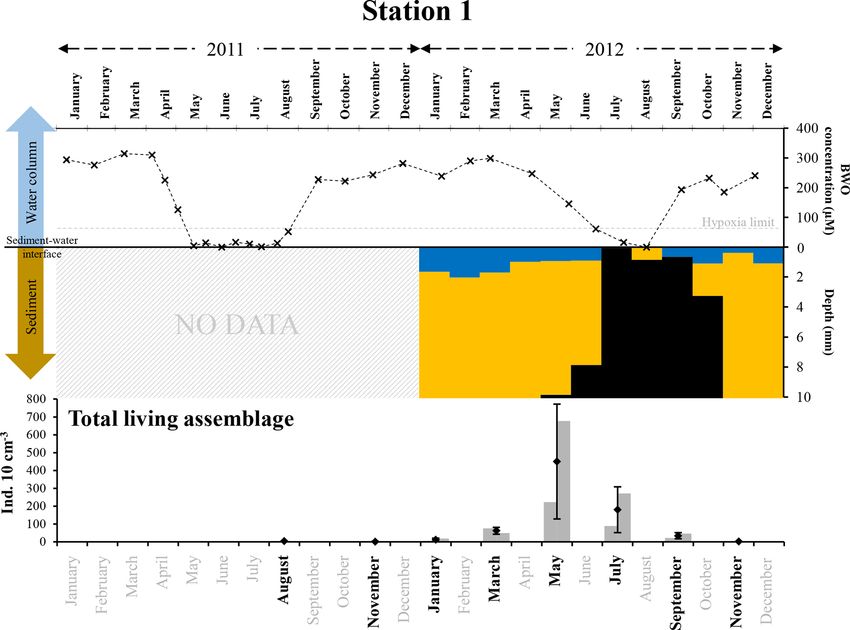
J. Richirt et al.: Foraminiferal community response to seasonal anoxia                                                     1417

pecies Ammonia tepida (probably Ammonia sp. T6) showed           into the possible moment(s) of reproduction or accelerated
minimal or no growth under anoxia. Conversely, Geslin et         growth in test size. The seasonal variability study of the
al. (2014) and Nardelli et al. (2014) suggested that, in the     foraminiferal community allows us (1) to better understand
same morphospecies, reproduction was strongly reduced,           the foraminiferal tolerance of seasonal hypoxia–anoxia with
but growth would not be affected by hypoxic and/or short         the presence of free H2 S in their microhabitat and (2) to ob-
anoxic events. Additionally, under low-oxygen conditions,        tain information about the responses of the various species
some species are able to shift to anaerobic metabolism (i.e.     to adverse conditions. This knowledge will be useful for the
denitrification; Risgaard-Petersen et al., 2006; Piña-Ochoa      development of indices assessing environmental quality (i.e.
et al., 2010a), to sequester chloroplast (i.e. kleptoplastidy;   biomonitoring) and may also improve palaeoecological inter-
Jauffrais et al., 2018), to associate with bacterial symbionts   pretations of coastal records (e.g. Murray, 1967; Gustafsson
(Bernhard et al., 2010) or to enter into a state of dormancy     and Nordberg, 1999).
(Ross and Hallock, 2016; LeKieffre et al., 2017).
   The highly peculiar environmental context of Lake Grev-
elingen offers an excellent opportunity to study this still      2     Material and methods
poorly known aspect of foraminiferal ecology.
   The conventional method to discriminate between live and      2.1    Studied area – environmental settings in the Den
dead foraminifera uses Rose Bengal, a compound which                    Osse Basin
stains proteins (i.e. organic matter). This method was pro-
posed for foraminifera by Walton (1952) and is based on the      Lake Grevelingen is a part of the former Rhine–Meuse–
assumption that “the presence of protoplasm is positive indi-    Scheldt estuary, in the southwestern Netherlands. This for-
cation of a living or very recently dead organism”. The au-      mer estuarine branch was turned into an artificial saltwater
thor already noted that this assumption implied that the rate    lake during the Delta Works project. In Lake Grevelingen,
of degradation of organic material should be relatively high.    the water circulation is strongly limited by the construction
Previous studies of living benthic foraminifera in environ-      of dams (in the early 1970s) and only a small sluice allows
ments subjected to hypoxia–anoxia were almost all based on       water exchanges with open seawater (i.e. very weak hydrody-
Rose Bengal-stained samples (e.g. Gustafsson and Nordberg,       namics). In the lake, development of bottom-water hypoxia–
1999, 2000; Duijnstee et al., 2004; Panieri, 2006; Schönfeld     anoxia occurs in the deepest part of the basin in summer (i.e.
and Numberger, 2007; Polovodova et al., 2009; Papaspy-           July–September) to early autumn (i.e. October–December;
rou et al., 2013). However, foraminiferal protoplasm may         Bannink et al., 1984; Hagens et al., 2015). In the litera-
remain stainable from several weeks to months after their        ture, the terminology and threshold values used to describe
death (Corliss and Emerson, 1990), especially under low dis-     oxygen depletion are highly variable (e.g. oxic, dysoxic, hy-
solved oxygen concentrations where organic matter degrada-       poxic, suboxic, microxic, postoxic; see Jorissen et al., 2007;
tion may be very slow (Bernhard, 1988; Hannah and Roger-         Altenbach et al., 2012). In this study we defined hypoxia
son, 1997; Bernhard et al., 2006). The Rose Bengal stain-        as a concentration of oxygen < 63 µmol L−1 (1.4 mL L−1 or
ing method is therefore not suitable for studies in environ-     2 mg L−1 ) whereas anoxia is defined as no detectable oxygen
ments affected by hypoxia–anoxia. Consequently, the results      (following Rabalais et al., 2010).
of foraminiferal studies in low-oxygen environments based           In Den Osse Basin, the nutrient input from external
on this method have to be considered with reserve. In order      sources is very low and pelagic–benthic coupling is essential,
to avoid this problem, we used CellTracker™ Green (CTG)          as already noted by de Vries and Hopstaken (1984). In 2012,
to recognise living foraminifera. CTG is a fluorescent probe     phytoplankton blooms occurred in April–May and July (Ha-
which marks only living individuals with cytoplasmic (i.e.       gens et al., 2015) in response to the increasing solar radiation
enzymatic) metabolic activity (Bernhard et al., 2006). Since     and nutrient availability in the water column following or-
metabolic activity stops after the death of the organism, CTG    ganic matter recycling in winter. This led to an increased food
should give a much more accurate assessment of the living        availability in the benthic compartment in the same periods.
assemblages at the various sampling times and thereby avoid      In general, Chl a concentrations in Den Osse Basin are be-
overestimation of the live foraminiferal abundances.             low 10 µg L−1 , excluding very short peaks during blooms in
   In this study, samples were collected in August and           April–May and July which did not exceed 30 µg L−1 in 2012
November 2011 and then every month through the year              (Hagens et al., 2015). Thermal stratification of the water col-
2012, at two different stations in the Den Osse Basin, with      umn and increased oxygen consumption due to organic mat-
two replicates dedicated to foraminifera. The two stations       ter input (i.e. from phytoplankton blooms) are both responsi-
were chosen in contrasted environments regarding water           ble for the development of seasonal bottom-water hypoxia–
depth (34 and 23 m, respectively) and duration of seasonal       anoxia in summer (i.e. July–September). Although euxinia
hypoxia–anoxia and sulfidic conditions. Living foraminiferal     (i.e. the presence of free H2 S in the water column) does not
assemblages were studied in the uppermost sediment and           occur in the Den Osse Basin due to cable bacterial activity
size distributions were determined in order to get insight       in winter, free H2 S is present in the uppermost layer of the

www.biogeosciences.net/17/1415/2020/                                                    Biogeosciences, 17, 1415–1435, 2020
1418                                               J. Richirt et al.: Foraminiferal community response to seasonal anoxia

sediment in summer (Seitaj et al., 2015). Summarising, in       Table 1. Sampling dates of the samples which were investigated for
the benthic ecosystem, increased food availability in summer    living foraminifera for stations 1 and 2. X: one core investigated; O:
is counterbalanced by strongly decreasing oxygen contents,      no core investigated.
sometimes accompanied by the presence of free sulfides in
the topmost sediment.                                                     Year     Month     Day     Station 1    Station 2
                                                                          2011     Aug         22      XX           XX
2.2    Field sampling                                                     2011     Nov         15      XX           XX
                                                                          2012     Jan         23      XX           XX
The two studied sites are located along a depth gradient in               2012     Mar         12      XX           XX
the Den Osse Basin of Lake Grevelingen. Both station 1                    2012     May         30      XX           XX
(51◦ 44.8340 N, 3◦ 53.4010 E) and station 2 (51◦ 44.9560 N,               2012     Jul         24      XX           XX
3◦ 53.8260 E) are located in the main channel, at 34 and 23 m             2012     Sep         20      XX           XX
depth, respectively (Fig. 1).                                             2012     Oct         18      O            XX
                                                                          2012     Nov          2      XX           XX
   Measurements of bottom-water oxygen (BWO) concentra-
                                                                          2012     Dec          3      O            XX
tions were performed at 2 m above the sediment–water inter-
face and are from Donders et al. (2012), whereas the data for
2012 were published in Hagens et al. (2015). Sediment cores
were collected monthly in 2012 using a single core gravity      492 nm/517 nm) and placed on micropalaeontological slides.
corer (UWITEC, Austria) using PVC core liners (6 cm in-         Only specimens that fluoresced brightly green were consid-
ner diameter, 60 cm length). All cores were inspected upon      ered living and were identified to the (morpho)species level
retrieval and only visually undisturbed sediment cores were     when possible. Since picking foraminifera under an epiflu-
used for further analysis (Seitaj et al., 2017). Oxygen pen-    orescence stereomicroscope is particularly time-consuming,
etration depth (OPD) and depth of free H2 S detection were      we decided to study samples only every 2 months for the
determined by Seitaj et al. (2015) using profiling microsen-    year 2012. At a later stage, in view of the large differences
sors for station 1. The data for station 2 (Supplement Ta-      in foraminiferal abundances between the samples of Septem-
ble S1) were acquired similarly and during the same cruises     ber and November 2012 at station 2, we decided to study the
but never published; for further details about the sampling     October and December 2012 samples as well for this station.
method, see Seitaj et al. (2015).                               The sampling dates investigated in this study are listed in Ta-
   Two replicate sediment cores dedicated to the                ble 1.
foraminiferal study were sampled in August and Novem-              Abundances were then standardised to a volume of
ber 2011 using the same gravity corer (UWITEC, Austria)         10 cm3 . The abundances of living foraminifera for each sam-
and then monthly throughout the year 2012 at the same           pling time and replicate are listed in Tables S2 and S3. The
sampling time as for BWO concentration and OPD and              mean abundance and standard deviation (x±SD) for the two
H2 S measurements in the sediment (see Seitaj et al., 2015).    replicates for each sampling date were calculated for both
Consequently, for 2012 at stations 1 and 2, OPD and H2 S        the total living assemblage and the individual species, as an
were measured in the sediment column at the same time as        indication of spatial patchiness.
foraminifera were sampled (Seitaj et al., 2015). For each
replicate, the uppermost centimetre (0–1 cm) of the core was    2.4   Taxonomy of dominant species
then transferred on board in a vial of 250 mL, and 30 mL of
seawater (at the same temperature as in situ) was added to      Four dominant species (> 1 % of the total assemblage)
the vial. Then we labelled the samples with CellTracker™        were present in our material: Ammonia sp. T6, Elphidium
Green CMFDA (CTG, 5-chloromethylfluorescein diacetate,          magellanicum (Heron-Allen and Earland, 1932), Elphidium
final concentration of 1 µmol L−1 following Bernhard et al.,    selseyense (Heron-Allen and Earland, 1911) and Trocham-
2006) and slowly agitated manually to allow the CTG dif-        mina inflata (Montagu, 1808). As we identified these species
fusion in the whole sample. Samples were then fixed in 5 %      on the basis of morphological criteria, we will use them as
sodium-borate-buffered formalin after 24 h of incubation in     “morphospecies”.
the dark.                                                          Concerning the genus Ammonia, two living specimens col-
                                                                lected at Grevelingen station 1 were molecularly identified
2.3    Sample treatment                                         (by DNA barcoding) as phylotype T6 by Bird et al. (2019).
                                                                At the same site, we genotyped seven other living Ammo-
All samples were sieved over 315, 150 and 125 µm meshes,        nia specimens, which were all T6. Their sequences were
and foraminiferal assemblages were studied in all three size    deposited in GenBank (accession numbers MN190684 to
fractions. Individuals were picked wet under an epifluores-     MN190690), and Supplement Fig. S1 shows scanning elec-
cence stereomicroscope (Olympus SZX12, light fluorescent        tron microscope (SEM) images of the spiral side and of the
source Olympus URFL-T, excitation/emission wavelengths:         penultimate chamber at 1000× magnification for four indi-

Biogeosciences, 17, 1415–1435, 2020                                                    www.biogeosciences.net/17/1415/2020/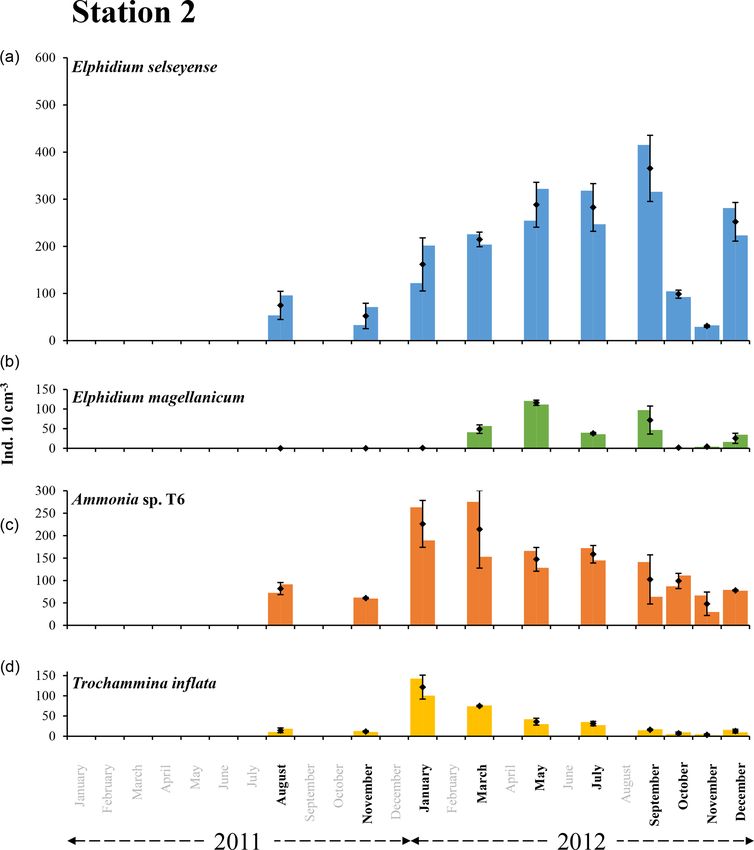
J. Richirt et al.: Foraminiferal community response to seasonal anoxia 1419
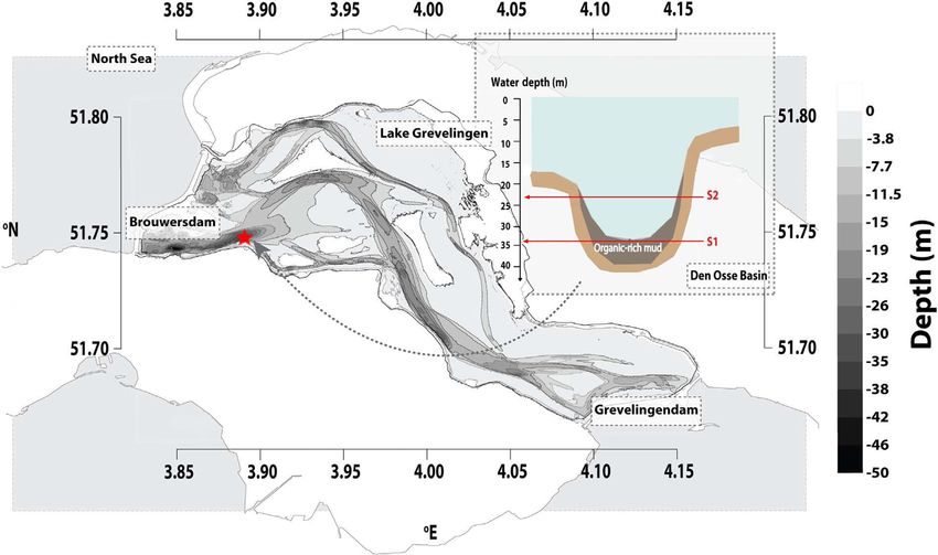
Figure 1. Map of Lake Grevelingen showing the location of the two sampled stations in the Den Osse Basin (red star). The transversal section
of the Den Osse Basin (top right) shows the depth at which station 1 (S1) and station 2 (S2) were sampled (34 and 23 m depth, respectively).
This figure was modified from Sulu-Gambari et al. (2016b).
viduals. A morphological screening based on the criteria pro- the number of small bosses in the umbilical region, which
posed by Richirt et al. (2019) confirmed that T6 accounts for we considered to be intraspecific variability. Consequently,
the vast majority (> 98 %) of Ammonia individuals, whereas we identified all our specimens as E. selseyense.
phylotypes T1, T2, T3 and T15 are only present in very small The specimens attributed to Trochammina inflata were
amounts (Table S3). also identified exclusively on the basis of morphological cri-
The specimens of Elphidium magellanicum were identi- teria, as no molecular data are available yet.
fied exclusively on the basis of morphological criteria, as
there are no molecular data available yet. This morphos- 2.5 Size distribution measurement
pecies, although rare, is regularly recognised in Boreal and
Lusitanian provinces of Europe (e.g. Gustafsson and Nord- In order to detect periods of increased growth and/or re-
berg, 1999; Darling et al., 2016; Alve et al., 2016). However, production, size measurements were performed on all sam-
as the type species was described from the Strait of Magellan ples of 2012. The measurements were made for all species
(Southern Chile), the European specimens may represent a (4176 individuals for station 1 and 19624 individuals for
different species and further studies involving DNA sequenc- station 2), and trochospiral species were all orientated spi-
ing of both populations are needed to confirm or disprove this ral side up prior to measurements. High-resolution images
taxonomic attribution (see Roberts et al., 2016). (3648 pixels × 2736 pixels) of all micropalaeontological
Elphidium selseyense has often been considered an slides were taken with a stereomicroscope (Leica S9i, 10×
ecophenotype of Elphidium excavatum (Terquem, 1875) and magnification) and individual measurements were processed
has been identified as E. excavatum forma selseyensis (e.g. using ImageJ software (Schneider et al., 2012, Fig. S2).
Feyling-Hanssen, 1972; Miller et al., 1982). Four living spec- Each individual was isolated (Fig. S2) and its maximum
imens were already sampled for DNA analysis at station 1 diameter was measured (i.e. Feret’s diameter). We repre-
and were all identified as the species E. selseyense (phylo- sented all size distributions using histograms with 20 µm
type S5, Darling et al., 2016). We only observed minor mor- classes (the best compromise between the total number of
phological variations in our material, especially concerning individuals and the size range (Fig. S3). As we only exam-
ined the size fractions >125 µm, our analysis mainly concerns
www.biogeosciences.net/17/1415/2020/ Biogeosciences, 17, 1415–1435, 20201420 J. Richirt et al.: Foraminiferal community response to seasonal anoxia
adult specimens and does not include juveniles. This limita- Total abundances then progressively decreased from May
tion should be kept in mind when interpreting the results. to September (x = 34.0 ± 17.0) and almost no foraminifera
Assuming that the size distribution was a sum of Gaussian were present in November (x = 1.6 ± 0.3).
curves, each of them representing a cohort, we tried to iden- At station 2, total abundances were comparatively low
tify the approximate mode for the Gaussian curves (i.e. co- in August and November 2011 (x = 174.0 ± 48.0 and x =
horts) using the changes in slope (i.e. inflexion points) of the 128.7 ± 25. ind. 10 cm−3 , respectively). In 2012, total abun-
second-order derivative of the total size distribution (Gam- dances were relatively high and stable from January to
mon et al., 2017). Unfortunately, this tentative attempt to dis- September (between x = 523.6 ± 30.7 and x = 604.8 ± 3.5),
tinguish cohorts by using a deconvolution method was not then decreased in October (x = 211.5 ± 8.0) and November
conclusive. The main problem was the lack of information (x = 91.1 ± 25.3), and finally increased again in December
concerning individuals smaller than 125 µm, so that our size (x = 377.9 ± 38.8).
distributions were systematically skewed toward small indi-
viduals. Because the identification of individual cohorts was 3.2 Dominant species
not successful, a study of population dynamics was not pos-
sible. For this reason, the data are only shown in Figs. S2 and At station 1, the major species were, in order of decreas-
S3. Nevertheless, the size distribution data give some clues ing abundances, Elphidium selseyense (Fig. 4a–b), Elphid-
concerning the possible moment(s) of reproduction or inten- ium magellanicum (Fig. 4c–d) and Ammonia sp. T6 (Fig. 4e–
sified test growth for the different species. g). In Fig. 4, we added Trochammina inflata (Fig. 4h–j) to
facilitate comparison with station 2, where this species is
2.6 Encrusted forms of E. magellanicum among the dominant ones. The “other species” account only
for 2.2 % of the total assemblage at station 1. The fact that
In our samples, we found abundant encrusted forms of E. they are well represented in some months (e.g. 26.3 % of
magellanicum at station 1 (May 2012) and station 2 (May, the assemblage in August 2011) is due to the extremely low
July, September and December 2012, Fig. 2). Most indi- number of individuals (see Fig. 3 and Table 2). At station 2,
viduals were totally encrusted (Fig. 2a), others only partly the dominant species, in order of decreasing abundances,
(Fig. 2b). These crusts were hard, firmly stuck to the shell were E. selseyense, Ammonia sp. T6, E. magellanicum and
(difficult to remove with a brush), thin (Fig. 2c–e) and rather T. inflata (Table 2). Here, “other species” account only for
coarse. In order to determine if the crust matrix is constituted 2.6 % of the total assemblage. Whereas E. selseyense and E.
of carbonate, we placed some specimens in microtubes and magellanicum were dominant species at both stations, both
exposed them to 0.1 M of EDTA (ethylenediaminetetraacetic Ammonia sp. T6 and T. inflata were present in much higher
acid) diluted in 0.1 M cacodylate buffer (acting as a carbon- abundances at station 2 compared to station 1, where the lat-
ate chelator). After an exposition of 24 h, we checked under a ter species was almost absent (Figs. 5–6).
stereomicroscope if the crust was still cohesive (no carbonate At station 1, only some very scarce individuals of E.
in the crust) or was disaggregated (crust contains carbonate). selseyense were observed in August and November 2011
(Fig. 5 and Table 2). In 2012, E. selseyense abundances were
very low in January and started to increase in March (x =
3 Results 23.9 ± 6.8), reaching maximal values in May (x = 336.5 ±
275.8). In July, values for E. selseyense were still high (x =
3.1 Total abundances of foraminiferal assemblages
162.0±121.5) and further decreased until an almost total ab-
Averaged total abundances varied between 1.1 ± 1.5 and sence in November 2012. No specimen of E. magellanicum
449.9 ±322.1 ind. 10 cm−3 for station 1 and between 91.1 ± was observed in 2011 (Fig. 5 and Table 2). The abundance
25.0 and 604.8 ±3.5 ind. 10 cm−3 for station 2 (Fig. 3 and Ta- of E. magellanicum was very low in January 2012, started to
ble 2). For every studied month, the total density was higher increase in March (x = 21.6 ± 11.0), reaching maximal val-
at station 2 than at station 1. The seasonal succession is very ues in May (x = 96.4 ± 47.3), and then strongly decreased in
different between the two sites (Fig. 3). Station 1 shows very July (x = 3.7±0.3). The species was absent from samples in
low total foraminiferal abundances for most months, con- September and November 2012. Ammonia sp. T6 was almost
trasting with much higher densities in May and July. Con- absent in August and November 2011 and present with very
versely, station 2 shows high total foraminiferal abundances few specimens in January 2012 (x = 3.2 ± 3.5). Maximum
throughout the year, with somewhat lower values in Novem- abundances were reached between March and July 2012
ber 2011 and October and November 2012 (Fig. 3). (ranging between x = 9.2 ± 6.5 and x = 12.9 ± 1.3). Then
At station 1, almost no individuals were present in August abundances rapidly decreased until the species was almost
(x = 3.4±1.3) and November 2011 (x = 1.1±1.5). In 2012, absent in November. Trochammina inflata was absent in 2011
total abundances were very low in January (x = 11.5 ± 9.3), and was only present in very low abundances from January
showed a slight increase in March (x = 62.1 ± 19.3) and to May and in September 2012.
reached a maximal abundance in May (x = 449.9 ± 322.1).
Biogeosciences, 17, 1415–1435, 2020 www.biogeosciences.net/17/1415/2020/J. Richirt et al.: Foraminiferal community response to seasonal anoxia 1421
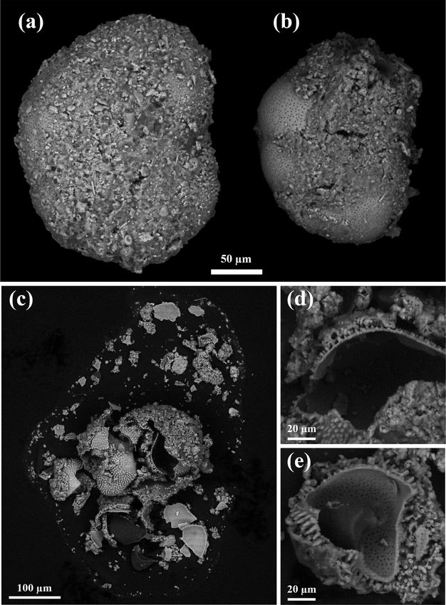
Figure 2. SEM images of fully encrusted specimen (a), partially encrusted specimen (b) and crushed encrusted specimen of Elphidium
magellanicum (c). Note the thinness of the crust and the spinose structures in (d) and (e).
At station 2, the two dominant species were E. selseyense nia sp. T6, abundances strongly increased between Novem-
and Ammonia sp. T6, which together always represented ber 2011 (x = 60.8 ± 1.5) and January 2012 (x = 226.2 ±
at least 70 % of the total assemblage (Fig. 6 and Table 2). 52.3) and then progressively decreased until the end of 2012
These two species showed a different seasonal pattern over (x = 48.1 ± 26.0 in November 2012). Trochammina inflata
the considered period. Abundances of E. selseyense were showed an analogous pattern to Ammonia sp. T6. Abun-
comparable in August (x = 74.8±29.8) and November 2011 dances strongly increased between November 2011 (x =
(x = 52.3±27.0) and then showed a progressive increase un- 11.8±1.8) and January 2012 (x = 121.5±29.8) and then pro-
til a maximum in September 2012 (x = 365.5±70.3). Abun- gressively decreased until very low abundances in November
dances then showed a sharp decrease in October and Novem- (x = 3.7 ± 3.0). E. magellanicum was completely absent in
ber (respectively x = 98.7 ± 8.5 and x = 30.9 ± 2.3) to in- August and November 2011, almost absent in January 2012
crease again in December (x = 252.2 ± 41.0). For Ammo- (x = 0.9 ± 0.3), and then suddenly increased until a max-
www.biogeosciences.net/17/1415/2020/ Biogeosciences, 17, 1415–1435, 20201422 J. Richirt et al.: Foraminiferal community response to seasonal anoxia
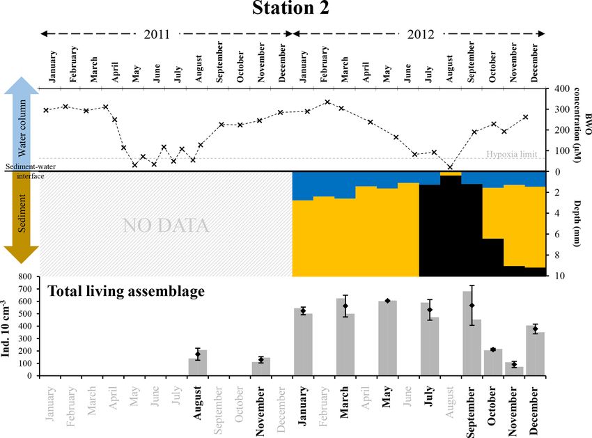
Figure 3. The grey bars represent the living foraminiferal abundances for the two replicates. The mean abundances (diamonds) and standard
deviations (black error bars) were calculated for the two replicates for stations 1 (34 m depth, a) and 2 (23 m depth, b). All abundance values
are for the 0–1 cm layer and were standardised to 10 cm3 . Months where foraminiferal communities were investigated are indicated in bold
(excluding October and December at station 1).
imum of x = 116.0 ± 6.5 in May. Abundances stayed rel- 4 Discussion
atively high in July (x = 37.8 ± 2.5) and September (x =
72.0 ± 35.8) and then drastically decreased until minimum 4.1 Tolerance of foraminiferal communities towards
numbers in October and November. Finally, like all other anoxia and free sulfide
species, E. magellanicum abundances increased again in De-
cember (x = 25.5 ± 13.0).
At station 1, bottom waters were hypoxic in July 2012 and
3.3 Encrusted forms of Elphidium magellanicum became anoxic in August (Fig. 8). Both in July and in Au-
gust, oxygen penetration into the sediment was null, whereas
After exposition to 0.1 M of EDTA diluted in 0.1 M cacody- it was 0.7±0.1 mm depth in September. In all 3 months (July
late buffer, the crusts remained cohesive, indicating that they to September 2012), sulfidic conditions were observed very
do not consist of carbonate and suggesting that they are com- close to the sediment–water interface (1 mm or less, Fig. 8
posed of sediment particles cemented by an organic matrix. and Table S1). In view of these results, the duration of anoxic
At station 1, encrusted forms of E. magellanicum were and sulfidic conditions in the uppermost sediment layer can
present in moderate proportions in May (26.8 % of the to- be estimated as 1 to 2 months (in July and August, Fig. 8).
tal E. magellanicum population, Fig. 7) and July (47.6 %); After the strong increase in foraminiferal densities in
the species disappeared thereafter. At station 2, encrusted May 2012, there was a decrease starting in July, leading
forms strongly dominated the E. magellanicum population to a near absence of foraminifera at station 1 in Novem-
from May (72.3 %) to December (88.0 %, Fig. 7). ber (Fig. 8). The most probable cause of the strong decline
of the foraminiferal community appears to be a prolonged
presence of sulfides in the foraminiferal microhabitat. How-
ever, the fact that foraminiferal abundances reached almost
Biogeosciences, 17, 1415–1435, 2020 www.biogeosciences.net/17/1415/2020/J. Richirt et al.: Foraminiferal community response to seasonal anoxia 1423
Table 2. Mean living foraminiferal absolute (ind. 10 cm−3 ) and relative abundances (percentage of the total fauna, in parentheses) of the
dominant species. Last column: absolute abundance of the total fauna.
Year Month Elphidium selseyense Ammonia sp. T6 Elphidium magellanicum Trochammina inflata Others Total
Station 1
2011 Aug 1.2 (36.8) 1.2 (36.8) 0.0 (0.0) 0.0 (0.0) 0.9 (26.3) 3.4
2011 Nov 0.5 (50.0) 0.4 (33.3) 0.0 (0.0) 0.0 (0.0) 0.2 (16.7) 1.1
2012 Jan 5.1 (44.6) 3.2 (27.7) 0.2 (1.5) 1.2 (10.8) 1.8 (15.4) 11.5
2012 Mar 23.9 (38.5) 12.9 (20.8) 21.6 (34.8) 1.4 (2.3) 2.3 (3.7) 62.1
2012 May 336.5 (74.8) 9.2 (2.0) 96.4 (21.4) 1.8 (0.4) 6.0 (1.3) 449.9
2012 Jul 162.0 (90.2) 10.3 (5.7) 3.7 (2.1) 0.0 (0.0) 3.5 (2.0) 179.5
2012 Sep 29.7 (87.5) 2.3 (6.8) 0.0 (0.0) 0.4 (1.0) 1.6 (4.7) 34.0
2012 Nov 1.1 (66.7) 0.4 (22.2) 0.0 (0.0) 0.0 (0.0) 0.2 (11.1) 1.6
Sum 560.0 (75.4) 39.8 (5.4) 121.8 (16.4) 4.8 (0.6) 16.4 (2.2) 742.9
Station 2
2011 Aug 74.8 (43.0) 82.1 (47.2) 0.0 (0.0) 14.7 (8.4) 2.5 (1.4) 174.0
2011 Nov 52.3 (40.7) 60.8 (47.3) 0.0 (0.0) 11.8 (9.2) 3.7 (2.9) 128.7
2012 Jan 161.8 (30.9) 226.2 (43.2) 0.9 (0.2) 121.5 (23.2) 13.3 (2.5) 523.6
2012 Mar 214.7 (38.2) 214.0 (38.1) 48.8 (8.7) 75.0 (13.3) 9.9 (1.8) 562.3
2012 May 288.2 (47.7) 147.1 (24.3) 116.0 (19.2) 36.1 (6.0) 17.3 (2.9) 604.8
2012 Jul 282.6 (53.2) 158.4 (29.8) 37.8 (7.1) 31.5 (5.9) 21.2 (4.0) 531.6
2012 Sep 365.5 (64.4) 102.4 (18.0) 72.0 (12.7) 16.1 (2.8) 11.5 (2.0) 567.5
2012 Oct 98.7 (46.7) 99.0 (46.8) 1.8 (0.8) 7.4 (3.5) 4.6 (2.2) 211.5
2012 Nov 30.9 (34.0) 48.1 (52.8) 4.1 (4.5) 3.7 (4.1) 4.2 (4.7) 91.1
2012 Dec 252.2 (66.7) 78.0 (20.6) 25.5 (6.7) 12.7 (3.4) 9.5 (2.5) 377.9
Sum 1821.8 (48.3) 1216.1 (32.2) 306.8 (8.1) 330.5 (8.8) 97.7 (2.6) 3773.0
zero only in September (about 2 months after the first oc- Our observations confirm the suggestion in previous stud-
currence of anoxic and sulfidic conditions in the upper sed- ies that the foraminiferal community is severely affected by
iment, in July) suggests that the presence of H2 S did not a long-term presence of H2 S in its habitat but does not show
cause instantaneous mortality, but that the disappearance of instant mortality. In fact, after a 66 d incubation in euxinic
the foraminiferal community was a delayed response, prob- conditions (a maximum of 11.9±0.4 µmol L−1 of H2 S in the
ably caused by inhibited reproduction and, eventually, in- overlying water) of foraminiferal assemblages collected at a
creased mortality. Inhibited reproduction has previously been 19 m deep site in the Adriatic Sea, Moodley et al. (1998a)
suggested as a response to hypoxic–short anoxic (Geslin et found a strong decrease in the total density of Rose Bengal-
al., 2014) and sulfidic conditions (Moodley et al., 1998b). stained foraminifera. After 21 d, living specimens were still
Such a time lag between a change in foraminiferal abun- observed, whereas after 42 and 66 d, the live checks (based
dances and changes in environmental parameters affecting on protoplasm movement) gave only negative results. Lan-
reproduction and/or growth of foraminifera has been sug- glet et al. (2013, 2014) performed an in situ experiment with
gested previously by Duijnstee et al. (2004). These authors closed benthic chambers at a 24 m deep site in the Gulf of
highlighted that the density patterns of some foraminiferal Trieste, in the Adriatic Sea. They observed a decrease in liv-
species showed a higher correlation with measured environ- ing foraminiferal density (labelled with CTG), but they also
mental parameters (e.g. oxygenation or temperature) when a found that almost all species survived after 10 months of
time lag of about 3 months was applied. anoxia and periodically co-occurring H2 S in the sediment
For 2011, at station 1, no pore-water O2 and H2 S measure- and overlying water. However, the duration of sulfidic con-
ments are available. However, severe hypoxia was observed ditions, which was estimated to be several weeks, could not
in the bottom waters from May to August, with anoxia in be assessed precisely (Metzger et al., 2014). The suggestion
June 2011 (Fig. 8). We therefore assume that, like in 2012, that short exposure to euxinic conditions is not directly lethal
anoxic and probably co-occurring sulfidic conditions were for foraminifera is confirmed by the experimental results of
responsible for the very low standing stocks in August and Bernhard (1993), who found that foraminiferal activity (as
November 2011 and January 2012. determined by ATP content) was not significantly affected
after 30 d exposure to euxinia (32.6 ± 8.6 % of active indi-
www.biogeosciences.net/17/1415/2020/ Biogeosciences, 17, 1415–1435, 20201424 J. Richirt et al.: Foraminiferal community response to seasonal anoxia Figure 4. SEM images of Elphidium selseyense in lateral (a) and peripheral (b) views; Elphidium magellanicum in lateral (c) and periph- eral (d) views; Ammonia sp. T6 in spiral (e), peripheral (f) and umbilical (g) views; and Trochammina inflata in spiral (h), peripheral (i) and umbilical (j) views. All scale bars are 50 µm. viduals, n = 174 in control conditions versus 29.5 ± 6.2 %, disappearance of the foraminiferal population was only par- n = 173 in sulfidic conditions). tial and not nearly as complete as in our study. After the 2011 hypoxia–anoxia, standing stocks at sta- At station 2, in 2012, hypoxia was only observed in Au- tion 1 only started to increase in March 2012, indicating a gust, when the OPD was zero, and sulfidic conditions were very long recovery time (about 6 months) of the foraminiferal observed in the superficial sediment (i.e. from 0.4 ± 0.2 mm faunas after a temporary near-extinction due to anoxic and downwards, Fig. 9, Table S1). Both in July and in Septem- sulfidic conditions. This confirms observations of relatively ber, oxygen penetrated more than 1 mm into the sediment long recovery times in the literature (e.g. Alve, 1995, 1999; (1.3 ± 0.4 and 1.2 ± 0.2 mm, respectively). However, free Gustafsson and Nordberg, 2000; Hess et al., 2005). For in- H2 S was still detected at about 1 mm depth in the sediment stance, Gustafsson and Nordberg (1999) showed that in the (1.1 ± 0.8 mm in July and 0.8 ± 0.2 mm in September). Al- Koljö Fjord, at comparable water depths, foraminiferal pop- though the sampling plan does not allow us to be very precise ulations responded with increased densities only 3 months about the duration of anoxic and sulfidic conditions, we can after a renewal of sea-floor oxygenation following hypoxic estimate their duration to be 1 month or less (Fig. 9). conditions in the bottom waters. However, in that case, the Biogeosciences, 17, 1415–1435, 2020 www.biogeosciences.net/17/1415/2020/
J. Richirt et al.: Foraminiferal community response to seasonal anoxia                                                                1425

Figure 5. The bars represent the living foraminiferal abundances for the two replicates for Elphidium selseyense (a), Elphidium magellanicum
(b), Ammonia sp. T6 (c) and Trochammina inflata (d) at station 1 in 2011 and 2012. The mean abundances (diamonds) and standard deviations
(black error bars) were calculated for the two replicates. All abundance values are for the 0–1 cm layer and were standardised to 10 cm3 .
Months when foraminiferal communities were investigated are indicated in bold. Scales were chosen in order to facilitate comparison with
station 2.

   Foraminiferal abundances showed a strong decrease in Oc-             Nevertheless, there was no replacement in the > 125 µm frac-
tober and November 2012, about 2 months after the presence              tion by growing juveniles, probably because reproduction
of anoxic and sulfidic conditions in the topmost part of the            was interrupted when H2 S was present in the foraminiferal
sediment (Fig. 9). Like at station 1, this temporal offset be-          microhabitat. A renewed recruitment after the last stage of
tween the presence of anoxia–sulfidic conditions at station 2           sulfidic conditions somewhere in September would then ex-
(in August) and the strong decrease in faunal densities may             plain why the faunal density in the > 125 µm fraction in-
be explained as a delayed response, mainly due to inhibited             creased again in December 2012 (Fig. S3).
reproduction during the anoxic–sulfidic event. If true, the                In 2011, at station 2, bottom waters oscillated between hy-
mortality of adults did not strongly increase in the months             poxic and oxic conditions between May and August (Fig. 9).
following the H2 S production in the uppermost sediment.                Although we have no measurements of H2 S in the pore

www.biogeosciences.net/17/1415/2020/                                                             Biogeosciences, 17, 1415–1435, 2020
1426                                                     J. Richirt et al.: Foraminiferal community response to seasonal anoxia

Figure 6. The bars represent the living foraminiferal abundances for the two replicates for Elphidium selseyense (a), Elphidium magellan-
icum (b), Ammonia sp. T6 (c) and Trochammina inflata (d) at station 2 in 2011 and 2012. The mean abundances (diamonds) and standard
deviations (black error bars) were calculated for the two replicates. All abundances values are for the 0–1 cm layer and were standardised to
10 cm3 . Months when foraminiferal communities were investigated are indicated in bold. Scales were chosen in order to facilitate comparison
with station 1.

waters for this year, it seems probable that bottom-water                   It is interesting to note that the foraminiferal densities ob-
hypoxia was accompanied by the presence of free H2 S                     served at station 2 were lower in August 2011 than in July or
very close to the sediment surface, strongly affecting the               September 2012. This may be a consequence of the repetition
foraminiferal communities. If we assume that, like in 2012,              of short hypoxic events in the bottom water between May and
rich foraminiferal fauna was present in May–July 2011 at                 August 2011 (probably associated with anoxia and maybe
both stations, the low faunal densities observed in August               H2 S in the uppermost part of the sediment), which possibly
and November 2011 could suggest that foraminifera may                    affected the foraminiferal community more substantially in
have also shown a delayed response to sulfidic conditions in             2011 than in 2012, when a hypoxic event was recorded in
2011.                                                                    August only.

Biogeosciences, 17, 1415–1435, 2020                                                            www.biogeosciences.net/17/1415/2020/
J. Richirt et al.: Foraminiferal community response to seasonal anoxia                                                        1427

Figure 7. Mean abundances (ind. 10 cm−3 ) of non-encrusted (grey) and encrusted forms (black) of Elphidium magellanicum in 2012, at
stations 1 (a) and 2 (b), with proportion of encrusted forms above each bar (%). Investigated months are indicated in bold.

   The important decrease in total standing stocks at station 2     4.2   Species-specific response to anoxia, sulfide and food
in October and November 2012 (Fig. 9) suggests that, in                   availability in Lake Grevelingen
spite of the shorter duration of anoxia and sulfide conditions
(compared to station 1; 1 month or less compared to 1 to
2 months), the foraminiferal faunas were still strongly af-         The comparison of the different seasonal patterns of the ma-
fected. However, at station 2, foraminiferal abundances in-         jor species at the two investigated stations allows us to draw
creased again in December 2012, suggesting a recovery time          some conclusions about interspecific differences in the re-
of about 2 months, which is likely much shorter than at sta-        sponse to seasonal anoxic and sulfidic conditions.
tion 1, where standing stocks in the > 125 µm fraction only            First, there is a clear faunal difference between the two
increased 6 months after the presence of anoxia and free sul-       stations. Station 1 is dominated by E. selseyense and E. mag-
fides.                                                              ellanicum while at station 2 these two taxa are accompanied
   Summarising, the foraminiferal communities of both sta-          by Ammonia sp. T6 and T. inflata. The latter species is al-
tions 1 and 2 seem strongly impacted by the anoxic and sul-         most absent at station 1, where Ammonia sp. T6 is present
fidic conditions developing in the uppermost part of the sedi-      with low densities. At first glance, the dominance of the two
ment in summer (i.e. July–September). However, at station 1,        Elphidium species at station 1 would suggest that they have
where anoxic and sulfidic conditions lasted for 1 to 2 months,      a greater tolerance of the seasonal anoxic and sulfidic condi-
the response is much stronger, leading ultimately (in Novem-        tions, which lasted much longer there. It is interesting to note
ber) to almost complete disappearance of the foraminiferal          that the temporal evolution of standing stocks at station 1 is
fauna. The delayed response at both stations shows that in-         different for the two Elphidium species. Elphidium magellan-
stantaneous mortality was limited and suggests that the de-         icum shows a strong drop in absolute density in July 2012, at
creasing standing stocks might rather be the result of inhib-       the onset of H2 S presence in the uppermost part of the sed-
ited reproduction and, eventually, increased mortality. Re-         iment, whereas the diminution of E. selseyense is more pro-
covery is much faster at station 2 (about 2 months) than at         gressive and the species disappears almost completely only
station 1 (about 6 months), probably because at station 1 (in       in November (Fig. 5). This strongly suggests that E. mag-
contrast to station 2) the foraminiferal extinction was nearly      ellanicum is more affected by increased mortality than E.
complete, and the site had to be recolonised (e.g. possibly by      selseyense in response to the combined effects of anoxic and
nearby sites or by the remaining few individuals) after reoxy-      sulfidic conditions. This hypothesis is confirmed by the pat-
genation of the sediment. At station 2, a reduced but signif-       terns observed at station 2, where the drop in standing stocks
icant foraminiferal community remained present, explaining          in October–November is also more drastic in E. magellan-
the faster recovery.                                                icum than in E. selseyense (Fig. 6).
                                                                       As mentioned earlier, certain species of foraminifera can
                                                                    use an anaerobic metabolism (i.e. denitrification; Risgaard-
                                                                    Petersen et al., 2006; Piña-Ochoa et al., 2010a), sequester
                                                                    chloroplasts (i.e. kleptoplastidy; Jauffrais et al., 2018), host
                                                                    bacterial symbionts (Bernhard et al., 2010) or enter dor-

www.biogeosciences.net/17/1415/2020/                                                       Biogeosciences, 17, 1415–1435, 2020
1428 J. Richirt et al.: Foraminiferal community response to seasonal anoxia Figure 8. The top panel represents bottom-water oxygen concentrations (µmol L−1 ) in 2011 and 2012 at station 1, from Donders et al. (2012) and Seitaj et al. (2017). The grey horizontal dotted line indicates the hypoxia limit (63 µmol L−1 ). The middle panel represents the depth (mm) distribution of the oxic zone (blue), absence of oxygen and sulfides (orange), and sulfidic zone (black) within the sediment in 2012, from Seitaj et al. (2015). The bottom panel shows the total living foraminiferal abundances for both replicates (grey bars), mean abundances (diamonds) and standard deviations (black error bars) calculated for the two replicates, for all investigated months (in bold) in 2011 and 2012. mancy (Ross and Hallock, 2016; LeKieffre et al., 2017) to them active for several days to weeks, in contrast to Ammo- deal with low-oxygen conditions. Concerning the species nia sp. T6 (Jauffrais et al., 2018). These active chloroplasts found in this study, although the presence of intracellular ni- could serve as an alternative source of oxygen and/or food trate was shown for Ammonia, denitrification tests yielded through photosynthesis (Bernhard and Alve, 1996) or an- negative results (Piña-Ochoa et al., 2010a; Nomaki et al., other metabolic pathway (Jauffrais et al., 2019) and thereby 2014). Similarly, the presence of active symbionts was previ- increase the capability of this species to survive anoxic ously suggested for Ammonia but never confirmed (Nomaki events. Although sequestration of chloroplasts was never in- et al., 2016; Bernhard et al., 2018). To our knowledge, den- vestigated for E. magellanicum, its abundant spinose orna- itrification or the presence of bacterial symbionts was never mentation in the umbilical region and in the vicinity of the shown for Elphidium either. In conclusion, a shift to an alter- aperture (Fig. 4c–d) suggests that this species is capable native anaerobic metabolism or an association with bacterial of crushing diatom frustules like some kleptoplastic species symbionts has never been shown conclusively for the domi- (Bernhard and Bowser, 1999; Austin et al., 2005). Hagens nant foraminiferal species found in Lake Grevelingen. et al. (2015) observed that the light penetration depth in the The greater tolerance of E. selseyense towards low-oxygen Den Osse Basin never exceeded 15 m in 2012, and therefore conditions could be explained by the fact that it is able photosynthesis by kleptoplasts (Bernhard and Alve, 1996) to sequester chloroplasts from ingested diatoms and keep appears unlikely for both our aphotic stations (34 and 23 m Biogeosciences, 17, 1415–1435, 2020 www.biogeosciences.net/17/1415/2020/
J. Richirt et al.: Foraminiferal community response to seasonal anoxia                                                                  1429

Figure 9. The top panel represents bottom-water oxygen concentrations (µmol L−1 ) in 2011 and 2012 at station 2, from Donders et al. (2012)
and Seitaj et al. (2017). The grey horizontal dotted line indicates the hypoxia limit (63 µmol L−1 ). The middle panel represents the depth
(mm) distribution of the oxic (blue), suboxic (orange, absence of oxygen and sulfides) and sulfidic (black) zones within the sediment in 2012.
The bottom panel shows the total living foraminiferal abundances for both replicates (grey bars), mean abundances (diamonds) and standard
deviations (black error bars) calculated for the two replicates, for all investigated months (in bold) in 2011 and 2012.

depth). However, other foraminifera from aphotic and anoxic              plain their stronger decrease in density at station 2 compared
environments such as deep fjords are kleptoplastic and use               to Ammonia sp. T6. Nevertheless, further studies about the
these kleptoplasts for a yet unknown purpose (Jauffrais et al.,          ability and mechanisms of the two Elphidium species to re-
2019).                                                                   sist anoxic–sulfidic conditions are necessary.
   Rather surprisingly, the drop in foraminiferal densities at              Another remarkable observation is that Ammonia sp. T6
station 2 in October–November, which we interpreted as a                 (and T. inflata) shows maximum densities in January–March,
delayed response to sulfidic conditions, is less strong for Am-          contrasting with the two Elphidium species, which have their
monia sp. T6 than for the two Elphidium species, suggesting              density maxima later in the year (May–September). This
that this species is less affected. However, this does not agree         temporal offset could possibly be explained by a difference
with our previous suggestion that the two Elphidium species              in preferential food source, with food particles available in
would be more tolerant to anoxic and sulfidic conditions. As             winter (January–March) being more suitable for Ammonia
already proposed by LeKieffre et al. (2017), Ammonia seems               sp. T6 (and T. inflata) and food particles available later in
to be able to deal with anoxia (up to 28 d, but with no sulfide)         the year, resulting from phytoplankton blooms, being more
by reducing its metabolic activity, but this ability was never           favourable for E. selseyense and E. magellanicum.
shown for Elphidium species. If E. selseyense and E. magel-                 In our study, for E. selseyense (and E. magellanicum),
lanicum are indeed unable to resist anoxia by reducing their             the continuous presence of a high proportion of small-sized
metabolism or by entering a dormancy state, this could ex-               specimens and progressively increasing densities between

www.biogeosciences.net/17/1415/2020/                                                              Biogeosciences, 17, 1415–1435, 2020
1430                                                   J. Richirt et al.: Foraminiferal community response to seasonal anoxia

January and September 2012 strongly suggest ongoing and              to a lower resistance to anoxia and free sulfides, but rather
continuous reproduction (Fig. S3a). Continuous reproduc-             due to an unfavourable seasonal succession of food availabil-
tion during the year has been described earlier for differ-          ity. Previous studies already suggested that hypoxic–anoxic
ent foraminiferal genera, such as Elphidium, Ammonia, Hay-           conditions coupled with increased food input from autumnal
nesina, Nonion and Trochammina (e.g. Jones and Ross, 1979;           phytoplankton blooms (composed of diatoms and dinoflag-
Murray, 1983, 1992; Cearreta, 1988; Basson and Murray,               ellates) would favour the development of E. magellanicum
1995; Gustafsson and Nordberg, 1999; Murray and Alve,                (Gustafsson and Nordberg, 1999). The fact that also at sta-
2000). Conversely, for Ammonia sp. T6, a decrease in densi-          tion 2 this species was mainly observed between March and
ties coupled with a rapid increase in overall test size between      September 2012 corroborates our conclusion of its depen-
March and May 2012 (small sized specimens remain present             dence on a specific food regime.
but in smaller proportions) could be indicative of a period of          Finally, encrusted forms of E. magellanicum were ob-
reduced recruitment (Fig. S3b).                                      served at both stations from May until the end of the year
    In fact, foraminifera exhibit a large range of feeding strate-   but were absent in the samples of March 2012. In view of
gies, with several species showing selective feeding with            the fact that the crusts consist mainly of organic matter, the
specific food particles (Muller, 1975; Suhr et al., 2003;            encrusted individuals appear to be specimens with preserved
Chronopoulou et al., 2019). Hagens et al. (2015) reported            feeding cysts. The precise functions of cysts observed around
that in Lake Grevelingen the phytoplankton composition was           foraminifera are not clear and include feeding, reproduction,
different between April–May and July 2012. In April–May,             chamber formation, protection or resting (Cedhagen, 1996;
the phytoplankton bloom was mainly composed of the hap-              Heinz et al., 2005). Concerning the cysts of E. magellan-
tophyte Phaeocystis globose (Scherffel, 1899), whereas it            icum described here, very similar observations have been
was dominated by the dinoflagellate Prorocentrum micans              made for Elphidium incertum at different locations (Norwe-
(Ehrenberg, 1834) in July. Elphidium was reported to be able         gian Greenland Sea and Baltic Sea in Linke and Lutze, 1993;
to feed on various food sources (e.g. diatoms, dinoflagel-           Koljö Fjord in Gustafsson and Nordberg, 1999; Kiel Bight in
lates, green algae; Correia and Lee, 2002; Pillet et al., 2011).     Polovodova et al., 2009). If we assume that encrusted spec-
However, diatoms are a major food source for kleptoplastic           imens indeed present the remains of feeding cysts, the ob-
species (Bernhard and Bowser, 1999), such as E. selseyense           servation of abundant encrusted specimens corroborates our
(Jauffrais et al., 2018; Chronopoulou et al., 2019). Ammo-           conclusion that the surface water phytoplankton bloom in
nia spp. seem able to feed on very diverse food sources              May 2012 (i.e. probably mainly Phaeocystis globosa) pro-
including microalgae, diatoms, bacteria or even metazoans            vided a food source particularly well suited to the nutritional
(Lee et al., 1969; Moodley et al., 2000; Dupuy et al., 2010;         preferences of this species.
Jauffrais et al., 2016; Chronopoulou et al., 2019). Recently,
Chronopoulou et al. (2019) showed different feeding prefer-
ences for Ammonia sp. T6 and E. selseyense in intertidal en-         5   Conclusions
vironments in the Dutch Wadden Sea. Although diatoms are
ingested by both species (but much more by E. selseyense),           In this study we examined the foraminiferal community re-
dinoflagellates were consumed by E. selseyense but not by            sponse to different durations of seasonal anoxia coupled with
Ammonia sp. T6. The latter species is also capable of feed-          the presence of sulfide in the uppermost layer of sediment
ing on metazoans by active predation (Dupuy et al., 2010).           at two stations in Lake Grevelingen. In both stations inves-
    These observations suggest that at station 2 the different       tigated, foraminiferal communities are highly impacted by
seasonal density patterns of Ammonia sp. T6 and the two              the combination of anoxia and H2 S in their habitat. The
Elphidium species are not the consequence of a large dif-            foraminiferal response varied depending on the duration of
ference in tolerance of anoxia–sulfides, but rather a differ-        adverse conditions and led to a near extinction at station 1,
ent adjustment to the seasonal cycle of food availability. At        where anoxic and sulfidic conditions were present for 1 to
station 1, the very low densities of Ammonia sp. T6 could            2 months, compared to a drop in standing stocks at sta-
possibly be explained by a recolonisation starting in January,       tion 2, where these conditions lasted for 1 month or less. At
when food conditions were favourable for this taxon (as tes-         both sites, foraminiferal communities showed a 2-month de-
tified by the strong density increase in January 2012 at sta-        lay in the response to anoxic and sulfidic conditions, sug-
tion 2). However, once a more abundant pioneer population            gesting that the presence of H2 S inhibited reproduction,
had developed (in March–May), food conditions may have               whereas mortality was not necessarily increased. The dura-
been no longer favourable for Ammonia sp. T6, explaining             tion of the subsequent recovery depended on whether the
why its density did not show a further increase. Conversely,         foraminiferal community was almost extinct (station 1) or re-
the food conditions may have become optimal for the two              mained present with reduced numbers (station 2). In the for-
Elphidium species, explaining their strong density increase          mer case, 6 months were needed for faunal recovery, whereas
between March and May 2012. If true, this would mean that            in the latter case, it took only 2 months. We hypothesise that
the lower densities of Ammonia sp. T6 would not be due               the dominance of E. selseyense and E. magellanicum at sta-

Biogeosciences, 17, 1415–1435, 2020                                                      www.biogeosciences.net/17/1415/2020/
You can also read