Topography-based statistical modelling reveals high spatial variability and seasonal emission patches in forest floor methane flux - Biogeosciences
←
→
Page content transcription
If your browser does not render page correctly, please read the page content below
Biogeosciences, 18, 2003–2025, 2021
https://doi.org/10.5194/bg-18-2003-2021
© Author(s) 2021. This work is distributed under
the Creative Commons Attribution 4.0 License.

Topography-based statistical modelling reveals high spatial
variability and seasonal emission patches in forest floor methane flux
Elisa Vainio1,2,3 , Olli Peltola4 , Ville Kasurinen1 , Antti-Jussi Kieloaho5 , Eeva-Stiina Tuittila6 , and Mari Pihlatie1,2,7
1 Institute for Atmospheric and Earth System Research (INAR)/Physics, University of Helsinki, Helsinki, Finland
2 Environmental   Soil Sciences, Department of Agricultural Sciences, University of Helsinki, Helsinki, Finland
3 Institute for Atmospheric and Earth System Research (INAR)/Forest Science, University of Helsinki, Helsinki, Finland
4 Climate Research Programme, Finnish Meteorological Institute, Helsinki, Finland
5 Natural Resources Institute Finland (LUKE), Helsinki, Finland
6 School of Forest Sciences, University of Eastern Finland, Joensuu, Finland
7 Viikki Plant Science Centre (ViPS), University of Helsinki, Helsinki, Finland

Correspondence: Elisa Vainio (elisa.vainio@helsinki.fi)

Received: 10 July 2020 – Discussion started: 10 September 2020
Revised: 5 February 2021 – Accepted: 8 February 2021 – Published: 19 March 2021

Abstract. Boreal forest soils are globally an important sink       summer (modelled range from −12.3 to 6.19 µmol m−2 h−1 )
for methane (CH4 ), while these soils are also capable of          compared to the autumn period (range from −14.6 to
emitting CH4 under favourable conditions. Soil wetness is          −2.12 µmol m−2 h−1 ), and overall the CH4 uptake rate was
a well-known driver of CH4 flux, and the wetness can be es-        higher in autumn compared to early summer. In the early
timated with several terrain indices developed for the pur-        summer there were patches emitting high amounts of CH4 ;
pose. The aim of this study was to quantify the spatial            however, these wet patches got drier and smaller in size to-
variability of the forest floor CH4 flux with a topography-        wards the autumn, changing their dynamics to CH4 uptake.
based upscaling method connecting the flux with its driv-          The mean values of the measured and modelled CH4 fluxes
ing factors. We conducted spatially extensive forest floor         for the sample point locations were similar, indicating that
CH4 flux and soil moisture measurements, complemented              the model was able to reproduce the results. For the whole
by ground vegetation classification, in a boreal pine forest.      site, upscaling predicted stronger CH4 uptake compared to
We then modelled the soil moisture with a random forest            simply averaging over the sample points. The results high-
model using digital-elevation-model-derived topographic in-        light the small-scale spatial variability of the boreal forest
dices, based on which we upscaled the forest floor CH4 flux.       floor CH4 flux and the importance of soil chamber placement
The modelling was performed for two seasons: May–July              in order to obtain spatially representative CH4 flux results.
and August–October. Additionally, we evaluated the num-            To predict the CH4 fluxes over large areas more reliably, the
ber of flux measurement points needed to get an accurate           locations of the sample points should be selected based on
estimate of the flux at the whole study site merely by av-         the spatial variability of the driving parameters, in addition
eraging. Our results demonstrate high spatial heterogeneity        to linking the measured fluxes with the parameters.
in the forest floor CH4 flux resulting from the soil mois-
ture variability as well as from the related ground vegeta-
tion. The mean measured CH4 flux at the sample points was
−5.07 µmol m−2 h−1 in May–July and −8.67 µmol m−2 h−1              1   Introduction
in August–October, while the modelled flux for the whole
area was −7.42 and −9.91 µmol m−2 h−1 for the two sea-             Methane (CH4 ) is an important and strong greenhouse gas,
sons, respectively. The spatial variability in the soil moisture   of which the largest natural source to the atmosphere is wet-
and consequently in the CH4 flux was higher in the early           lands (Kirschke et al., 2013; Saunois et al., 2016). While ox-
                                                                   idation by hydroxyl radicals (OH) in the atmosphere forms

Published by Copernicus Publications on behalf of the European Geosciences Union.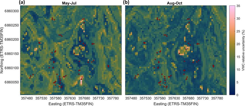
2004                                                           E. Vainio et al.: Spatial variability in forest floor methane flux

the largest natural CH4 sink, boreal upland forests are consid-     also been reported to emit CH4 (e.g. Gauci et al., 2010;
ered to be a globally important terrestrial sink due to soil CH4    Machacova et al., 2016), contribute to the ecosystem-level
oxidation by methanotrophs (Kirschke et al., 2013; Saunois          flux. As the sources and sinks within the ecosystems are not
et al., 2016). The sink role of upland forests is well in agree-    adequately known or accounted for, forest floor CH4 fluxes
ment with the current paradigm, where methanotrophy only            require revisit and thorough estimation in all the climatic
occurs in oxic conditions, while methanogenesis requires            zones, especially in the boreal zone, where the climate warm-
anoxic conditions. However, CH4 -producing methanogens              ing is pronounced, and at both “upland” and “lowland” sites
are found to be universal also in well-drained upland soils         with an emphasized focus on the local topography.
(Angel et al., 2012), which is linked to the findings that             In order to precisely estimate the forest floor CH4 flux
methanogenesis can occur in anaerobic microenvironments             variation, determining the variability of the driving param-
within oxic soils (Angel et al., 2011; Angel et al., 2017).         eters, i.e. particularly soil moisture, is needed. Airborne li-
   As the availability of oxygen is the main controller for         dar (light detection and ranging) is an active remote-sensing
CH4 dynamics, soil moisture and water table level are among         method that can be used to observe the vegetation and terrain
the most important factors regulating CH4 formation as well         (Jaboyedoff et al., 2012) and that is very effective in forests
as consumption in soils. When soils become inundated with           (Korpela et al., 2009). Soil moisture is highly dependent on
water, the environment often turns anoxic, thus creating            the terrain topography, like elevation and slope, and there are
favourable conditions for methanogenesis – however, there           several digital elevation model (DEM)-derived digital terrain
are likely notable time lags between the start of inundation        indices developed for estimating soil wetness (Ågren et al.,
and methanogenesis, complicating the analyses of depen-             2014). When combining lidar-based measurements with the
dencies between these processes. Consequently, upland bo-           variables of interest measured on-site, it is possible to create
real forest soils (Lohila et al., 2016; Matson et al., 2009;        landscape-scale maps of the studied variable, such as forest
Savage et al., 1997), and even the whole forest ecosystems          floor–soil CH4 exchange (Kaiser et al., 2018; Sundqvist et
(Shoemaker et al., 2014), can shift from CH4 consumption            al., 2015; Warner et al., 2019) or soil moisture (Kemppinen
to CH4 emission, or vice versa, following the soil water con-       et al., 2018).
ditions. Besides soil moisture, temperature is known to be             In this study, we used a relatively high number of mea-
an important factor in regulating CH4 fluxes, by controlling        surement points (60 points in an area of ca. 10 ha) in or-
several microbial reactions, including methanogenesis and           der to fully cover the small-scale spatial variability in the
methanotrophy (Luo et al., 2013; Praeg et al., 2017; Yvon-          CH4 flux and its driving forces. Similar types of studies us-
Durocher et al., 2014). Similarly to microbial production of        ing chamber measurements are rarely based on more than 20
CH4 , non-microbial CH4 production in soil (Jugold et al.,          measurement points yet assuming that they are representa-
2012; B. Wang et al., 2013) has also been linked to soil wa-        tive of a larger area. The aim of this study was (1) to quantify
ter conditions and temperature: the alternation of soil drying      the spatial variation in the forest floor CH4 exchange, (2) to
and re-wetting (Jugold et al., 2012), as well as high tempera-      quantitatively link small-scale spatial variability in the up-
ture (Jugold et al., 2012; B. Wang et al., 2013), enhances the      land forest floor CH4 exchange to the topography, soil mois-
non-microbial CH4 emissions.                                        ture, and vegetation structure, and (3) to detect the poten-
   Spahni et al. (2011) estimated global CH4 emissions from         tial CH4 -emitting patches (hotspots). We combined the CH4
occasionally wet mineral soils to be 58–93 Tg CH4 yr−1 , ac-        flux data with the driving parameters to produce an upscaled
counting for 11 %–18 % of the global emissions (depending           ecosystem-scale forest floor CH4 flux of the area. Only a
on the scenario). Annual CH4 flux of upland sites is evalu-         few studies have applied a similar approach (Kaiser et al.,
ated to range from −23 to 73 g CH4 m−2 yr−1 (Treat et al.,          2018; Warner et al., 2019), among them Kaiser et al. (2018)
2018). Nevertheless, aerated soils are generally considered         in boreal coniferous forest, emphasizing the novelty of this
to consume CH4 , while CH4 production via methanogene-              research.
sis in occasionally wet mineral soils is neglected from most
of the global models (Curry, 2007; Saunois et al., 2016). Fur-
thermore, the division of ecosystems into upland and wetland        2     Materials and methods
sites is to some extent imprecise and thus subject to contin-
uous discussion, as the intrinsic definition of “upland” may        2.1    Site description and experimental design
vary from study to study. Usually the concept of “upland” is
relative to the surrounding topography, and there is no uni-        In order to quantify the spatial variability, we conducted for-
form limit for e.g. minimum elevation.                              est floor CH4 flux and soil moisture measurements at 60 sam-
   The upland forest CH4 emission estimates are partly based        ple points covering an area of ca. 10 ha around the SMEAR
on observations above forest canopies (Flanagan et al., 2020;       II station (Station for Measuring Ecosystem-Atmosphere Re-
Mikkelsen et al., 2011; Shoemaker et al., 2014). They fur-          lations) in Hyytiälä, southern Finland (61◦ 510 N, 24◦ 170 E;
ther raise the question whether these CH4 emissions origi-          160–180 m a.s.l.). The station is a combined ecosystem and
nate only from the forest floor or whether trees, which have        atmospheric site in the ICOS (Integrated Carbon Observa-

Biogeosciences, 18, 2003–2025, 2021                                                    https://doi.org/10.5194/bg-18-2003-2021
E. Vainio et al.: Spatial variability in forest floor methane flux                                                               2005

tion System) network. The measurements were performed
during two growing seasons (2013 and 2014). The site was
regenerated in 1962 by prescribed burning and sowing of Pi-
nus sylvestris (Scots pine) (Hari and Kulmala, 2005). The
mineral soils in the area are mostly podzols, while there are
also some small peaty depressions and some areas with al-
most no topsoil on the bedrock (Ilvesniemi et al., 2009).
The soil at the site is rather shallow (5–150 cm) on top of
the bedrock (Hari and Kulmala, 2005). Annual mean tem-
perature and precipitation in 1981–2010 were 3.5 ◦ C and
711 mm, respectively (Pirinen et al., 2012).
   In addition to P. sylvestris as a dominating tree species,
prevalent species at the site are Picea abies (Norway spruce),
Betula pendula (silver birch), and Betula pubescens (downy
birch), together with some Juniperus communis, Salix sp.,
and Sorbus aucuparia (Ilvesniemi et al., 2009). The ground
vegetation is mainly composed of Vaccinium myrtillus (Euro-
pean blueberry) and Vaccinium vitis-idaea (lingonberry), to-
gether with e.g. Deschampsia flexuosa, Trientalis europaea,
Maianthemum bifolium, Linnaea borealis, and Calluna vul-
                                                                 Figure 1. Locations of the sample points (diamonds) at the study
garis (Ilvesniemi et al., 2009). The most common mosses are
                                                                 site. The hilltop sample points are coloured light green, and the rest
Pleurozium schreberi, Dicranum polysetum, Polytrichum sp.,
                                                                 are pink. The cartographic depth-to-water (DTW) index is showed
Hylocomium splendens, and Sphagnum sp. (Ilvesniemi et al.,       on top of the aerial image, lighter colour indicating a higher DTW,
2009).                                                           i.e. drier soil.
   To represent the heterogeneity in vegetation and soil mois-
ture, we located 6 sample points in the highest area on top
of the hill and 54 at all the wind directions from the hill-     chamber measurements were always performed 15–155 min
top (Fig. 1). The sample points were identified based on the     before the opaque chamber at the same sample points. As
cardinal and intermediate directions from the centre of the      there was no significant difference in the flux between the
studied area (the main mast of SMEAR II), thus having eight      chamber types, the data were merged (transparent chambers
sectors (north–north-east sector N–NE, north-east–east NE–       were used in 14 % of the measurements in the final data).
E, etc.), accompanied by an Arabic numeral (1–9) depending       All the chambers were equipped with a fan to ensure mixing
on the distance from the centre of the study area (e.g. sam-     of the chamber headspace air and a vent tube to minimize
ple point SE–S-1 being the closest to the centre at the sector   pressure disturbances inside the chamber. The collars were
SE–S). The hilltop sample points are located in the sectors      installed in May 2013 1 week before the beginning of the
N–NE, NE–E, and E–SE, but they are labelled with the letter      measurements (except for the hilltop chambers, which were
H instead of the directions.                                     installed already in 2002 – Pihlatie et al., 2007) at a depth
                                                                 of ca. 5 cm to avoid cutting of tree roots and to minimize the
2.2   Flux measurements                                          sideways diffusion in the soil affecting the flux (Hutchinson
                                                                 and Livingston, 2001). Fine quartz sand was added to the
The flux measurements were conducted with non-steady-            edges of the collars to ensure the installation.
state non-flow-through static chambers (Livingston and              The chambers were closed for 35–45 min, and five samples
Hutchinson, 1995) at each sample point, principally follow-      were taken during each closure. Small parts of the closures
ing the guidelines compiled in the ICOS protocol (Pavelka et     (10 % of the final data) were 75 min with seven samples,
al., 2018). The majority of the measurements were conducted      due to a separate study on N2 O fluxes. The samples were
with opaque aluminium or stainless steel chambers. The hill-     taken with 65 mL syringes (BD Plastipak™, Becton, Dickin-
top chambers were on average 0.027 m3 , including the col-       son and Company, New Jersey, USA), and samples of 20 mL
lar (depending on the collar height and the vegetation inside    were inserted into glass vials (12 mL, Labco Exetainer® ,
the chamber), covering a forest floor area of 0.40 × 0.29 m.     Labco Limited, Wales, UK) after flushing the vial with the
The rest of the chambers were on average 0.102 m3 , cov-         sample. The samples were stored in the dark at +5 ◦ C be-
ering an area of 0.55 m × 0.55 m. Part of the measurements       fore analyses with a gas chromatograph (GC) (7890A, Ag-
were conducted with transparent chambers made of FEP (flu-       ilent Technologies, California, USA) equipped with a flame
orinated ethylene propylene) foil and PTFE (polytetrafluo-       ionization detector (for details, see Pihlatie et al., 2013). The
roethylene) tape in order to test the effect of photosyntheti-   chamber headspace air temperature was also recorded (DT-
cally active radiation (PAR) on the CH4 flux. The transparent    612, CEM Instruments, Shenzhen Everbest Machinery In-

https://doi.org/10.5194/bg-18-2003-2021                                                   Biogeosciences, 18, 2003–2025, 2021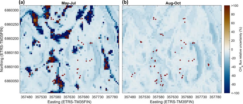
2006                                                           E. Vainio et al.: Spatial variability in forest floor methane flux

dustry Co. Ltd., Shenzhen, China) during the measurements           −0.146 and +0.244 µmol m−2 h−1 for the smaller chambers,
for the flux calculation.                                           calculated by the linear fit. While in general linear fit tends to
   Measurements from the hilltop sample points were con-            underestimate the chamber fluxes (Pihlatie et al., 2013), re-
ducted every 2–9 weeks between 21 March and 20 December             garding small fluxes, exponential fitting is more prone to er-
2013 and every 2–7 weeks between 10 April and 27 Novem-             rors and over-parameterization, and the relationship between
ber 2014. The other 54 sample points were measured on av-           linear and exponential flux values is more variable (Korki-
erage every 3–4 weeks between 29 May and 13 September               akoski et al., 2017; Pedersen et al., 2010). Thus it is recom-
2013 and between 20 May and 10 December 2014. In prac-              mended to select between linear or non-linear fitting depend-
tice, all the hilltop sample points were always measured dur-       ing on the concentration data (Korkiakoski et al., 2017; Ped-
ing one day, while the rest of the sample points (or as many        ersen et al., 2010). We used linear fits for all the fluxes that
as possible) were measured during a 5 d period. In May–             were below the MQL.
October, each sample point was measured on average every                After filtering the data, the final flux data included in total
22 d. Some of the sample points were measured significantly         723 measurements, of which 344 are from year 2013 and 379
more often than others, each being measured 7–23 times dur-         from year 2014. There were 5–21 measurements from each
ing the 2-year campaign with a median of 13 measurements            sample point, with a median of 11 measurements per point. In
per sample point. The most active measurement period was            the final data set, 467 fluxes were calculated with exponential
June–August for both years.                                         fit and 256 with linear fit, of which 184 were below the MQL.

2.3    Flux calculation                                             2.4   Environmental variables

The procedure in flux calculations included (1) filtering out-      We measured soil moisture (volumetric water content) in the
liers from raw concentration data, (2) calculating fluxes using     A horizon (ca. 5 cm depth) manually at the sample points
linear and non-linear functions and estimating goodness-of-         (except for the hilltop area) simultaneously with the flux
fit (GOF) parameters for the fluxes, (3) flagging the fluxes        measurements (ThetaProbe ML2x with HH2 Moisture Me-
based on the method quantification limit (MQL; Corley,              ter, Delta-T Devices Ltd, Cambridge, UK). The soil moisture
2003), (4) applying GOF criteria to flux data, and (5) cre-         was calculated as an average of three recordings at a sam-
ating final flux data.                                              ple point. In the hilltop area, the soil moisture was measured
   We removed the outliers from the CH4 mixing ratio data           continuously with a Time Domain Reflectometer (TDR-100,
by using a robust regression analysis that uses iteratively         Campbell Scientific Inc., Utah, USA).
reweighted least squares with a bisquare weighting function            Soil temperature in the A horizon was logged next to each
(Holland and Welsch, 1977) and by setting a weight limit to         sample point (except for the hilltop) eight times a day from
0.87 and discarding all points below this limit as outliers. The    June to October in 2013 and from April/May to October in
fluxes were calculated from the outlier-filtered raw data using     2014 with Thermochron iButton devices (Maxim Integrated
both linear and exponential fits (for the calculation, see Pih-     Products, California, USA). In the hilltop area, the A horizon
latie et al., 2013). The exponential fit parameters were based      soil temperature was recorded automatically at five locations
on 17th-order Taylor power series expansion (Kutzbach et            by silicon temperature sensors (KTY81-110, Philips, Nether-
al., 2007).                                                         lands) at 10 min intervals. In the analysis, we used daily av-
   Firstly, decreasing CO2 in an opaque chamber or CO2 flux         erage soil temperatures of the flux measurement days at each
below the MQL indicate a possible problem with the mea-             sample point. For May–June in 2013, when the iButtons were
surement, e.g. leaking chamber, and thus these measurements         not yet installed, we used the hilltop soil temperature data,
were omitted. For the CH4 fluxes that were above the MQL,           as the temperature was rather consistent at all the sample
the following GOF criteria must be met for the flux to be           points (average temperature on 12–30 June 2013 at the sam-
included in the final flux data: normalized root mean square        ple points ranged from 10.8 to 13.4 ◦ C).
error (NRMSE) below 0.2 and the coefficient of determina-              In addition to the continuous recordings of soil temper-
tion (R 2 ) above 0.7. The fluxes below the MQL were ac-            ature and moisture, we used air temperature at 4.2 m height
cepted in the final data as such, without applying the NRMSE        (Pt100 sensors with radiation shields by Metallityöpaja Toivo
and R 2 criteria, as neither of these GOF parameters works          Pohja) and precipitation (Vaisala FD12P weather sensor at
for close-to-zero fluxes. Furthermore, if the CH4 mixing ra-        18 m height) measured at the SMEAR II station.
tio was >10 ppm in the beginning of the closure, the flux
was omitted. Finally, there was one exceptionally large CH4         2.5   Ground vegetation of the sample points
emission which was omitted from the final data set.
   The MQL of the GC was 0.10 ppm for CH4 and                       The composition of ground vegetation in 54 sample points
151 ppm for CO2 (calculated according to Corley, 2003).             (all except the hilltop points) was described by estimating
The CH4 fluxes below the MQL were between −3.74 and                 projection cover of each plant species with the help of a
+2.38 µmol m−2 h−1 for the larger chambers and between              frame divided into 0.1 × 0.1 m sectors. Cover less than 5 %

Biogeosciences, 18, 2003–2025, 2021                                                     https://doi.org/10.5194/bg-18-2003-2021
E. Vainio et al.: Spatial variability in forest floor methane flux                                                         2007

was marked as 3 %. To group the sample points based on            Finland, 2/2019), biomass of foliage (for pine, spruce, and
their plant composition, we performed a two-way indicator         broadleaf trees) and tree volumes (for pine, spruce, and birch)
species analysis (TWINSPAN), a divisive clustering method         (16 × 16 m; Multi-source National Forest Inventory, Natural
using TWINSPAN for Windows version 2.3 (Hill and Šmi-             Resources Institute Finland, 2015; Mäkisara et al., 2019),
lauer, 2005). We used moss species as indicators because          subsoil types (basal deposit at a depth of 1 m) (16 × 116 m;
their distribution is generally more strongly related to soil     superficial deposits 1 : 20 000/1 : 50 000, Geological Survey
moisture than the distribution of clonal vascular plants typi-    of Finland, 2015), and peated soil areas (16 × 16 m; topo-
cal of boreal forests (e.g. Hokkanen, 2006). For a robust re-     graphic database, National Land Survey of Finland, 8/2018).
sult we excluded species whose frequency was less than 3.         In addition, we calculated the following topographic indices
Based on the plant species composition in 54 sample points,       from the DEM: topographic wetness index (TWI; Beven and
we created four vegetation groups. To visualize the varia-        Kirkby, 1979), terrain ruggedness index (TRI; Riley et al.,
tion within and between the groups, we performed canoni-          1999), slope, and cartographic depth-to-water index (DTW;
cal correspondence analysis (CCA) where vegetation groups         Murphy et al., 2007) (Appendix A, Figs. A1–A4). Before
from TWINSPAN were used as environmental variables. Be-           calculating the indices, the DEM was pre-processed to be
fore CCA, detrended correspondence analysis (DCA) was             hydrologically correct by using the TopoToolbox “carve” op-
conducted to decide between linear and unimodal methods.          tion (Schwanghart and Kuhn, 2010). TWI was calculated as
Canoco 5.11 (Šmilauer and Lepš, 2014) was applied for both        a natural logarithm of the ratio between the specific catch-
analyses.                                                         ment area (contributing area per unit contour length) and tan-
                                                                  gent of the local slope. The upslope catchment area was cal-
2.6   Statistical analyses                                        culated using multiple flow direction algorithms (Freeman,
                                                                  1991; Schwanghart and Kuhn, 2010), and local slope was
Multiple-group comparisons were performed with one-way            calculated using adjacent points in the DEM. The calcula-
ANOVA and two-group comparisons with a t test, when               tions were made with TopoToolbox. Following the recom-
Levene’s test indicated equal variances, and distribution was     mendations by Ågren et al. (2014), TWI was calculated from
normal or sample size large enough. When groups had un-           the coarse-resolution (16 m) DEM and scaled back to a finer
equal variances, we used Welch’s ANOVA (analysis of vari-         5 m grid with bilinear interpolation, since Ågren et al. (2014)
ance) together with a Games–Howell test as a post hoc test.       found that TWI calculated from the coarse grid represented
When comparing two groups with unequal variances, we              the soil moisture better than when calculated from a finer
used Welch’s t test or Satterthwaite’s approximation. When        grid. The other indices were calculated from the DEM with
groups had equal variances but distribution was non-normal        5 m resolution. TRI was calculated using the gdaldem pro-
or sample size was very small, we used Kruskal–Wallis, fol-       gram, which is part of the Geospatial Data Abstraction Li-
lowed by Bonferroni correction for pairwise comparisons.          brary (GDAL). TRI describes the amount of elevation differ-
   Spearman’s correlation coefficients were calculated to         ence between adjacent cells in a DEM grid and hence pre-
study the relationships between the CH4 fluxes and the en-        sumably has a low value on flat hilltops and depressions. The
vironmental/topographical parameters at the camber loca-          flow channel networks in the study domain used for the DTW
tions. Spearman’s correlation was also performed between          calculations were estimated from the DEM using a 1 ha flow
the CH4 flux, soil moisture, and soil temperature time-series     initiation threshold (Ågren et al., 2014), and then the DTW
data, as the correlations were not linear. Soil temperature can   values were calculated using the r.cost function of GRASS
increase both CH4 emissions and uptake, by increasing the         GIS, where the terrain slope raster map was used as a cost
activity of the soil microbes, and thus we used absolute flux     layer (e.g. Murphy et al., 2007). DTW can be considered to
values when examining the effect of the temperature.              describe the elevation difference to the nearest open water
   Welch’s t test, Welch’s ANOVA, and Kruskal–Wallis, ac-         location derived from the DEM.
companied by the post hoc tests, were performed with SPSS
(IBM SPSS Statistics 24, New York, USA). Regular one-way          2.8   Modelling the soil moisture and the CH4 flux to the
ANOVA, Levene’s tests, and correlation analyses were per-               site
formed with MATLAB (R2017b/R2018b, MathWorks, Nat-
ick, Massachusetts, USA). The statistical analyses were as-       We used a random forest (RF) algorithm (Breiman, 2001) to
sessed at a significance level of p
2008 E. Vainio et al.: Spatial variability in forest floor methane flux ability of soil moisture has been shown to be difficult even sampling points. This approach is similar to the one used in with larger data sets than the one used here (Kemppinen et e.g. Peltola et al. (2019) and Aalto et al. (2018). al., 2018). All 60 sample points, for which data were tempo- After modelling the soil moisture to the whole study do- rally averaged for the two separate periods (on average seven main, the forest floor CH4 flux was modelled as well using and five measurements for each point during May–July and the produced soil moisture raster map along with the maps of August–October, respectively), were used in RF model de- topographic metrics used to develop the RF model for CH4 velopment. RF is a machine-learning algorithm that can be flux. used to generalize complex dependencies between driving variables and a target variable. Here, our RF models con- 2.9 Evaluating the representability of chamber sisted of a large ensemble of regression trees, which were measurements trained each with a separate random subsample of available data. The output from the RF model is an average of output The representability of CH4 flux chamber measurements was from all the trees separately – and hence the algorithm ap- evaluated by comparing the average of CH4 fluxes measured plies the bootstrap aggregation (bagging) method, which de- at n chamber locations against the mean CH4 flux modelled creases the noise of the prediction. The model for soil mois- for the whole study domain with the RF modelling approach ture was developed using four drivers (TWI, slope, DTW, (Sect. 2.8). The aim of this analysis was to evaluate how and TRI) and for CH4 flux using five drivers (soil moisture, many chamber measurement locations are needed to get an TWI, slope, DTW, and TRI), selected based on the corre- accurate estimate of landscape-level flux by only averaging lations (Appendix A, Table A1, Figs. A5–A6). MATLAB over the measured chamber data without any upscaling with (R2018b, MathWorks, Natick, Massachusetts, USA) func- e.g. RF algorithms. The mean RF-modelled CH4 flux is used tion TreeBagger was used for developing the RF models in as a reference as it accounts for the soil heterogeneity. The this study. Each trained forest consisted of 300 regression CH4 fluxes measured at n chamber locations were selected trees, and a minimum of two samples were allowed in a split at random and averaged. This was repeated for a maximum node. Values for these hyperparameters were selected based of 500 times for each n and mean absolute bias between these on initial testing using out-of-bag errors and the minimum estimates, and the reference was calculated as a metric for the number of observations per tree leaf was set to two, due to representability of n chamber locations. the limited amount of data available. However, the number of variables randomly sampled as candidates at each split 3 Results was not changed from its default value (one-third of the total number of variables). 3.1 Ground vegetation at the sample points The predictive performance of the developed RF models was evaluated using distance-blocked leave-one-out cross- The most common vascular species growing in the sam- validation. In this method, one RF model is developed for ple points were V. vitis-idaea (48 out of 54 studied sample each sample point location, and the training data consist points), V. myrtillus (45 points), Equisetum sylvaticum, and of data measured further than the selected distance (here L. borealis, followed by M. bifolium and T. europaea. The 30 m) from the sample point location in question, while the most prevalent mosses were P. schreberi (34 points), Poly- rest of the data (i.e. data originating from closer than 30 m) trichum commune (29 points), Sphagnum spp. (28 points), are utilized as independent validation data. This way the D. polysetum, and H. splendens. possible spatial autocorrelations in the data did not inflate The four vegetation groups were named based on their the cross-validation metrics (Appendix A, Figs. A7–A9). dominant mosses. (1) The Sphagnum group included 15 sam- Blocked cross-validation has been proposed as an appropri- ple points that had over 50 % Sphagnum coverage (except ate cross-validation strategy for data showing e.g. spatial au- for one point) and no P. schreberi. Distinctive species were tocorrelations (Roberts et al., 2017), and it has been used in also E. sylvaticum, Carex digitata, and P. commune, which all some prior flux upscaling exercises (Peltola et al., 2019). Sta- are typical of peatland forest. (2) The Sphagnum–Pleurozium tistical metrics used in evaluating model predictive perfor- group is an intermediary group between the swampy and mance included mean bias, fraction of variance explained by drier forest areas, with some Sphagnum but also P. schreberi the model (R 2 ), Nash–Sutcliffe model efficiency (NSE), and in all 13 of its sample points. Sample points in the remaining root mean squared error (RMSE). The uncertainty of the up- two groups do not include any Sphagnum but species char- scaled soil moisture and CH4 flux, however, was estimated acteristic of upland forests. Sample points in (3) the Pleuroz- by developing 100 RF models with a random subset (70 %) ium group have typically more than 10 % P. schreberi, while of available data, and the variability (standard deviation) over the sample points in (4) the Hylocomium group have less this ensemble was used as an uncertainty estimate. The un- P. schreberi and usually more than 80 % H. splendens, which certainty estimate describes the robustness of the soil mois- is related to slightly higher fertility. D. polysetum was most ture and CH4 flux dependence on the drivers identified by the common in the Pleurozium group, and some of the Pleuroz- RF model but likely also the effect of the distribution of the ium group had high L. borealis coverage. V. vitis-idaea and Biogeosciences, 18, 2003–2025, 2021 https://doi.org/10.5194/bg-18-2003-2021
E. Vainio et al.: Spatial variability in forest floor methane flux                                                              2009

                                                                          The mean soil moisture of the sample points ranged from
                                                                      0.09 (±0.03 SD) m3 m−3 (sample point NE–E-3) to 0.89
                                                                      (±0.12 SD) m3 m−3 (E–SE-6). Furthermore, there was a sig-
                                                                      nificant difference in the mean soil moisture between the sea-
                                                                      sons May–July and August–October (0.25 (±0.06 SD) and
                                                                      0.18 (±0.05 SD) m3 m−3 , respectively, SMEAR II contin-
                                                                      uous measurements, or 0.35 (±0.28 SD) and 0.29 (±0.22
                                                                      SD) m3 m−3 , respectively, at the sample points on measure-
                                                                      ment days; p
2010 E. Vainio et al.: Spatial variability in forest floor methane flux
Figure 4. The soil moisture (volumetric water content, m3 m−3 ) (a,
b) and the measured CH4 flux (µmol m−2 h−1 ) (c, d) of the dif-
ferent vegetation groups in May–July and August–October. The as-
Figure 3. The relationship between the mean of the measured soil
terisks indicate the mean values, triangles indicate the medians, and
moisture (volumetric water content, m3 m−3 ) and the mean of the
the whiskers show the 25th and 75th percentiles. Statistically signif-
measured CH4 flux (µmol h−1 m−2 ) at the sample points (Spear-
icant differences (pE. Vainio et al.: Spatial variability in forest floor methane flux 2011
moisture in May–July was 0.25 m3 m−3 (±0.12 SD) and in
August–October 0.23 m3 m−3 (±0.09 SD) (Table 2). The
mean of the modelled values at the sample point locations
(0.33 and 0.29 m3 m−3 in May–July and August–October, re-
spectively) were similar to the measured mean values (0.33
and 0.28 m3 m−3 in May–July and August–October, respec-
tively), while the modelled averages for the whole area were
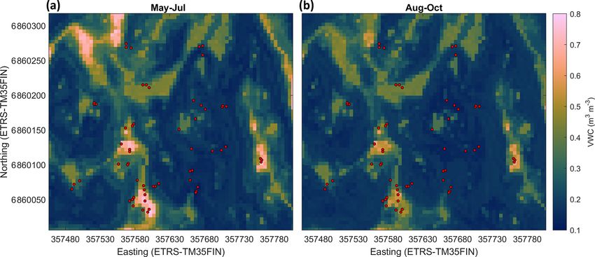
slightly lower for both seasons (Table 2). Based on the RF-
modelled soil moisture, the site was mostly rather dry in
2013–2014, with some wetter areas where the soil moisture
was above 0.5 m3 m−3 (Fig. 6). The modelling results indi-
cated that the wet areas were wetter and wider in May–July
(Fig. 6a) than in August–October (Fig. 6b), which follows
from the measured soil moisture (see Sect. 3.2). In May–
July 5 % of the area was wet (soil moisture >0.5 m3 m−3 ),
whereas in August–October only ca. 1 % of the area could
be considered wet. The RF model predicted high soil mois-
ture for topographical depressions and flat areas, which were
specified by low DTW, slope, and TRI, and high TWI val-
ues. The soil moisture was spatially more variable in early
Figure 5. Fluxes of CH4 (µmol CH4 m−2 h−1 ) from the sample summer than in autumn. The relative uncertainty of the up-
point groups. Mean values are represented with triangles and me- scaled soil moisture was on average 12 % and 9.6 % dur-
dians with circles, and the whiskers show the 25th and 75th per-
ing May–July and August–October, respectively (Fig. 7).
centiles.
The uncertainty increased with the predicted soil moisture,
yet during May–July the wettest locations (soil moisture
Table 1. Statistical metrics outlining the predictive performance of above 0.65 m3 m−3 ) had on average smaller relative uncer-
the RF model for the soil moisture during the two seasons. The met-
tainty than the locations with intermediate (soil moisture be-
rics were calculated using a distance-blocked cross-validation tech-
tween 0.4 and 0.65 m3 m−3 ) wetness (5.5 % and 9.7 %, re-
nique.
spectively). This indicates that the RF model was able to bet-
ter constrain the moisture variability at wet depressions and
R2 NSE RMSE Bias
at very dry locations than in areas with intermediate wetness,
(m3 m−3 ) (m3 m−3 )
using the drivers used to develop the model (see Sect. 2.7).
May–July 0.51 0.18 0.17 0.014 Based on cross-validation, the agreement between the
August–October 0.26 −0.25 0.17 0.015 upscaled and measured CH4 fluxes at the different cham-
ber locations was moderate (R 2 = 0.26 and R 2 = 0.39 for
May–July and August–October, respectively) (Table 3; see
was −8.01 ± 3.22 µmol m−2 h−1 , and in August–October, also Appendix Fig. A9). Note that the upscaling had dif-
−10.3 ± 5.04 µmol m−2 h−1 . ficulties especially in representing the tails of the CH4
flux distribution (strong uptake/emission), which has an
3.4 Modelled soil moisture and CH4 flux at the site influence on the cross-validation metrics. The mean bias
(upscaled–measured) was 0.10 and −0.10 µmol m−2 h−1 for
The performance of the RF model in predicting soil moisture the May–July and August–October periods, respectively.
variability in the study domain is outlined with the statistical The modelled CH4 flux of the whole studied area was
metrics shown in Table 1 (see also Appendix Fig. A8). These between −12.3 and 6.17 µmol m−2 h−1 in May–July, with
metrics were calculated against independent validation data a mean flux of −7.42 µmol m−2 h−1 (±3.26 SD) (Table
and hence are suitable for assessing the predictive perfor- 2). In August–October, the flux ranged from −14.6 to
mance of the model. R 2 values were 0.51 and 0.26 for May– −2.12 µmol m−2 h−1 , with a mean of −9.91 µmol m−2 h−1
July and August–October, indicating that the model was able (±2.73 SD) (Table 2). The modelled fluxes resulted in
to describe the spatial variation in soil moisture more accu- stronger CH4 uptake than averaging the flux measure-
rately during the early summer period. The RMSE and mean ments of 60 sample points (Table 2). The upscaling demon-
bias in the model prediction were similar during both peri- strated some CH4 -emitting patches in the early summer
ods. (Fig. 8a), which shifted to CH4 uptake in the autumn
The modelled soil moisture of the whole studied area (Fig. 8b). The emission patches covered approximately 3 %
ranged in May–July from 0.11 to 0.79 m3 m−3 and in of the study area, and the flux of the emitting areas was
August–October from 0.12 to 0.65 m3 m−3 . The mean soil 0.029–6.19 µmol m−2 h−1 in May–July. Omitting the emis-
https://doi.org/10.5194/bg-18-2003-2021 Biogeosciences, 18, 2003–2025, 20212012 E. Vainio et al.: Spatial variability in forest floor methane flux
Figure 6. Modelled soil moisture (volumetric water content, m3 m−3 ) at the site in May–July (a) and August–October (b). The red circles
show the sample points.
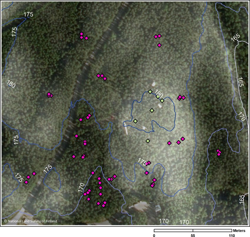
Figure 7. Relative uncertainty of the modelled soil moisture (volumetric water content, %) at the site in May–July (a) and August–October
(b). The relative uncertainty was defined as the standard deviation of the results of individual random forest models in the RF model ensemble
divided by the modelled soil moisture (see Sect. 2.8). The red circles show the sample points.
sion patches from calculation would result in ca. 4 % stronger In order to evaluate the number of sample points needed
mean CH4 uptake in May–July. The soil moisture of the emit- to produce an accurate estimate of the landscape-level for-
ting cells was between 0.39 and 0.79 m3 m−3 in May–July, est floor CH4 flux, we compared mean CH4 flux from 1 to
with a mean of 0.60 m3 m−3 . In autumn the emission patches 60 randomly picked sample points with the mean of the up-
were drier, the soil moisture of these areas being 0.38– scaled flux (Sect. 2.9). Based on this comparison, we state
0.65 m3 m−3 with a mean of 0.48 m3 m−3 (±0.065 SD), and that with approximately 15–20 randomly selected sample
the CH4 flux was between −5.31 and −2.12 µmol m−2 h−1 points similar accuracy was achieved to averaging over all
with a mean of −3.67 µmol m−2 h−1 (±0.615 SD). The rel- the sample points (Fig. 10). This finding held irrespective of
ative uncertainties of the upscaled forest floor CH4 fluxes the study period investigated.
were larger at the wet depressions than in dry areas (Fig. 9);
however, the absolute uncertainties were lower. The upscaled
CH4 flux uncertainty showed a similar spatial pattern during 4 Discussion
both periods. The lower absolute uncertainty at wet depres-
sions was due to lower variability of the measured CH4 fluxes 4.1 Drivers and spatial variation of the CH4 flux in the
between measurement locations at wet spots. Note that these two seasons
uncertainty maps represent only the uncertainty stemming
from the upscaling procedure with the RF model. Cross- We performed spatially extensive CH4 flux measurements
validation metrics presented above are better for evaluating from the forest floor, covering different soil moisture con-
the overall uncertainty, which includes e.g. uncertainties re- ditions and vegetation types in the area, and combined the
lated to possibly biased sampling locations. measured data with remote-sensing tools in order to unravel
the spatial variation in the forest floor CH4 flux within the
Biogeosciences, 18, 2003–2025, 2021 https://doi.org/10.5194/bg-18-2003-2021E. Vainio et al.: Spatial variability in forest floor methane flux 2013
Table 2. The means (±standard deviation) and ranges of the measured and modelled CH4 fluxes (µmol m−2 h−1 ) and the measured and
modelled soil moisture (m3 m−3 ) for the two seasons (May–July and August–October).
Measured (sample points) Modelled (sample points) Modelled (whole area)
Mean SD Range of sample Mean SD Range Mean SD Range
point means
CH4 flux (µmol m−2 h−1 )
May–July −5.07 (±11.0) −20.2 to 58.5 −5.84 (±4.67) −11.6 to 6.19 −7.42 (±3.26) −12.3 to 6.19
August–October −8.67 (±5.12) −24.1 to −1.31 −8.51 (±3.80) −13.0 to −2.12 −9.91 (±2.73) −14.6 to −2.12
Soil moisture (m3 m−3 )
May–July 0.33 (±0.24) 0.066 to 0.92 0.33 (±0.20) 0.11 to 0.77 0.25 (±0.12) 0.11 to 0.79
August–October 0.28 (±0.18) 0.089 to 0.86 0.29 (±0.16) 0.12 to 0.65 0.23 (±0.091) 0.12 to 0.65
Table 3. Statistical metrics outlining the agreement between upscaled and measured CH4 fluxes at different chamber locations.
R2 NSE RMSE Bias
(µmol m−2 h−1 ) (µmol m−2 h−1 )
May–July 0.26 −0.96 9.5 0.1
August–October 0.39 −0.50 4.0 −0.1
terrain. We accomplished this by generating random forest forest ground vegetation have been suggested to contribute
(RF) models to map the soil moisture and the CH4 flux at the to CH4 exchange, and the effect may vary between species
boreal forest site. Our results demonstrate that even though (Halmeenmäki et al., 2017; Maier et al., 2017; Praeg et al.,
the forest floor is mainly a sink of CH4 , as expected for the 2017), yet the studies focusing on forest ground vegetation
mainly dry upland pine forest, the CH4 flux at the site is are still rare. Also, different tree species can affect the soil
highly heterogeneous. conditions and thus the forest floor CH4 flux, for example
In our study, the soil moisture was the most important driv- through soil chemical properties or nutrient conditions (Reay
ing force in the spatial variability of the CH4 fluxes, whereas et al., 2005). While soil moisture also undergoes short-term
soil moisture is highly driven by topography. In previous temporal changes resulting from weather conditions, ground
studies, soil moisture and TWI have also been identified as vegetation is an important indicator of long-term soil condi-
the main factors affecting the soil CH4 fluxes from a spa- tions and their spatial variability. Thus it can be used as a
tial perspective (Kaiser et al., 2018; Warner et al., 2019). rough in situ estimate of the CH4 flux when planning the lo-
Furthermore, soil moisture and vegetation are strongly in- cations of the measurement plots, as demonstrated by this
terconnected: while topography-driven soil moisture controls study. The Pleurozium group was the most prevalent veg-
vegetation (Moeslund et al., 2013), vegetation can also affect etation type within our sample points, representing typical
soil moisture via e.g. evapotranspiration (Dunn and Mackay, ground vegetation of boreal pine forests. The mean CH4 flux
1995) or rooting strategies (Milly, 1997). As the soil mois- of the sample points in the Pleurozium group was close to the
ture is affected by topography, vegetation, and soil proper- modelled seasonal mean fluxes.
ties, it can have high spatial variability (Rosenbaum et al., Even though the difference in mean soil moisture between
2012). Based on our results, there was high variation in the the studied seasons was not large, the wet areas were wet-
CH4 fluxes even within the sample point groups, which may ter and wider in May–July than in August–October, result-
be explained by different vegetation groups among adjacent ing in CH4 emissions in May–July, while in the dry areas
sample points. the CH4 uptake increased substantially between the seasons.
Our vegetation classification was mostly based on mosses, This suggests that either the activity of CH4 -oxidizing bacte-
and the connection to soil moisture was expected. Conse- ria seems to increase towards autumn in the dry areas, which
quently, the groups differed in their soil moisture, and, fur- could be linked to soil temperature being at the highest level
thermore, in their CH4 flux. However, while the soil mois- in August, or that the activity of methanogens in the deeper
ture did not differ between the Pleurozium group and the soil (or microsites) decreases due to drying. Previously re-
Hylocomium group, there was a significant difference in the ported results indicate that there is a local optimal soil mois-
CH4 fluxes in autumn, suggesting that the ground vegeta- ture for CH4 oxidation, and in boreal forest soils the oxi-
tion as such may affect the CH4 flux. Some plant species of dation of CH4 decreases when the soil moisture increases
https://doi.org/10.5194/bg-18-2003-2021 Biogeosciences, 18, 2003–2025, 20212014 E. Vainio et al.: Spatial variability in forest floor methane flux Figure 8. Modelled forest floor CH4 flux (µmol m−2 h−1 ) at the site in May–July (a) and August–October (b). (Values below zero indicate uptake and values above zero emission). The red circles show the sample points. Figure 9. Relative uncertainty of the modelled forest floor CH4 flux (%) at the site in May–July (a) and August–October (b). The relative uncertainty was defined as the standard deviation of the results of individual random forest models in the RF model ensemble divided by the modelled CH4 flux (see Sect. 2.8). The red circles show the sample points. (Billings et al., 2000), whereas low soil water content as such gust 2006 and June 2007) (Skiba et al., 2009) and −4.6 does not remarkably decrease CH4 uptake of boreal forests’ µmol m−2 h−1 (between April and November in 2008) (Aal- mineral soils (Saari et al., 1998). The oxidation of CH4 has tonen et al., 2011). This may be explained by stronger CH4 been discovered to be at the lowest level in late spring and uptake due to drier years. Flux data processing techniques early summer and most effective in autumn by both the high- may also cause discrepancies between this and prior studies, affinity and low-affinity methanotrophs (Reay et al., 2005). as the widely used linear flux calculation method has been Similarly to our results, upscaling of CH4 fluxes across hill- demonstrated to underestimate the CH4 fluxes by on aver- slope transects in a temperate deciduous forest by Warner et age 33 % in a chamber intercomparison study (Pihlatie et al., al. (2019) demonstrated CH4 emissions from low-elevation 2013). Skiba et al. (2009) and Aaltonen et al. (2011) used the areas in early summer and uptake in late summer – moreover, linear flux calculation method, whereas here we mainly used the magnitudes of the upscaled fluxes were similar to our a non-linear method. From a wider perspective, the mean upscaling results. In contrast, Aaltonen et al. (2011) found CH4 fluxes obtained from both the measurements (mean the CH4 uptake to be stronger in May–June compared to late of all the sample points: May–July −5.07, August–October summer and autumn at the hilltop of the SMEAR II site (in −8.67 µmol m−2 h−1 ) and the modelling (May–July −7.74, 2008) (Aaltonen et al., 2011). August–October −10.0 µmol m−2 h−1 ) in our study were in Our results at the hilltop showed higher CH4 uptake (mean line with previously reported forest floor CH4 fluxes from −8.01 µmol m−2 h−1 in May–July and −10.3 µmol m−2 h−1 boreal and temperate coniferous forests (−0.62 to −15 µmol in August–October) compared to the previous forest floor CH4 m−2 h−1 , Jang et al., 2006). CH4 flux measurements from the same hilltop area, report- ing a mean CH4 flux of −7.0 µmol m−2 h−1 (between Au- Biogeosciences, 18, 2003–2025, 2021 https://doi.org/10.5194/bg-18-2003-2021
E. Vainio et al.: Spatial variability in forest floor methane flux                                                             2015

                                                                    572 mm in 2014; average 711 mm for 1981–2010) suggests
                                                                    that the emission patches can be larger in wetter years. The
                                                                    temporal variability in soil moisture is mainly driven by me-
                                                                    teorological forcing and is suggested to be greater at loca-
                                                                    tions with intermediate soil moisture than at the extremely
                                                                    dry or wet locations and in the topsoil compared to deeper
                                                                    soil layers (Rosenbaum et al., 2012). In our study, the mean
                                                                    soil moisture decreased between the early summer and au-
                                                                    tumn in the two wettest vegetation groups but stayed at the
                                                                    same level in the two driest groups, while the mean CH4
                                                                    flux showed increasing uptake in all the vegetation groups
                                                                    between the two seasons. This demonstrates that the tempo-
                                                                    ral changes in soil moisture affect mainly the wet areas of the
                                                                    forest in our study, while the driest areas tend to remain dry,
                                                                    probably due to the well-drained and shallow topsoil on top
                                                                    of a bedrock.
                                                                       Based on our results, most of the wet plots were located in
                                                                    the areas with sandy or gravelly till as subsoil, while the ar-
Figure 10. Mean absolute bias in the measured forest floor CH4
                                                                    eas with bedrock close to the soil surface (max. 1 m soil) had
flux estimated from a random subset of the sample points. Mean
upscaled CH4 flux was used as a reference. (Max. 500 sample point
                                                                    lower soil moisture. However, the sample points E–SE-4–6
combinations were calculated.)                                      were located in a depression with a ca. 0.6 m deep peat layer,
                                                                    which was on top of a bedrock area according to the subsoil
                                                                    map. Praeg et al. (2017) also reported bedrock type affect-
4.2   Hotspots of CH4 emissions                                     ing the CH4 flux, probably through soil properties, rooting of
                                                                    plants, plant species, and microbial composition – however,
At the site, there was one anomalous water-filled sample            for better understanding more research is needed.
point (SW–W-3), from which the CH4 emissions were at the
same level as emissions reported from a nearby fen site (Li         4.3   Representativeness of sample point locations
et al., 2016; Rinne et al., 2007, 2018). Even though the lo-
cation of SW–W-3 had the highest water table level, some of         In our study, the great advantage is the large number of sam-
the other sample points also had a water table at or close to       ple points, resolving the small-scale spatial variability of the
the soil surface. However, we did not measure as high CH4           forest floor CH4 flux. Some previous studies have upscaled
emissions from any of the other sample points – excluding           CH4 flux using similar types of approaches across complex
SW–W-3, the highest emission was 1 order of magnitude               terrains with measurements from slope transects (Kaiser et
smaller than the highest emission from SW–W-3. Out of the           al., 2018; Warner et al., 2019). The site studied here repre-
10 highest emissions measured, 7 were from SW–W-3 and               sents a typical commercial pine forest of the boreal areas,
the rest from sample points E–SE-4–6 in another peaty area.         and the results are thus scalable to a large area of similar
These substantially higher emissions from SW–W-3 com-               types of forests in the boreal zone. The mean CH4 flux ob-
pared to other sample points with high soil water content and       tained from all the sample points was rather close to but
equally high Sphagnum coverage may be related to the joint          slightly higher than the upscaled CH4 flux obtained from the
effect of these two factors. The Sphagnum mosses thrive in          model, indicating that the sample points covered the spatial
wet conditions, where CH4 is also produced, and most of             variation of both the soil moisture and CH4 flux in the area.
the Sphagnum mosses growing in Finland are demonstrated             However, while the mean values can be insufficient to tell a
to support methanotrophic bacteria (Larmola et al., 2010),          full story (i.e. it misses the spatial and temporal variability),
which therefore naturally reduces the potential CH4 emis-           comparison of means is important when targeting an accurate
sions from Sphagnum-covered wet areas. However, it may              landscape-scale CH4 budget. Based on our results, we state
be that while the Sphagnum-associated methanotrophs may             that 15–20 sample points are needed to reliably cover an area
reduce the CH4 emissions from many of the sample points,            of comparable size of a typical boreal commercial forest, de-
they may not be active during the highest water level at SW–        manding however carefully designed placement in order to
W-3.                                                                cover the spatial heterogeneity. Yet an area with higher to-
   Our results indicate that the observed spatial hotspots of       pographical variation may require more sample points. Our
CH4 emissions seem to be prone to temporal variation, de-           conclusion of the recommended number of sample points is
pending on the soil water status, affecting also the size of        slightly lower compared to the ICOS measurement proto-
these patches. The measurement years being drier than the           col, which recommends having at least 25 points at a site
long-term average (annual precipitation 576 mm in 2013 and          when using manual chambers (Pavelka et al., 2018). In addi-

https://doi.org/10.5194/bg-18-2003-2021                                                    Biogeosciences, 18, 2003–2025, 2021
2016 E. Vainio et al.: Spatial variability in forest floor methane flux
tion, our results suggest that, in August–October, only three likely include variables linked to plant activity and/or soil or-
randomly picked sample points would be as representative a ganic carbon storage, since these are related to the amount
sampling of the whole area as 15–20 sample points in May– of substrates available for the microbes. Even though we cre-
July, which was probably due to smaller spatial variability in ated the model based on the correlations with several poten-
the CH4 flux in autumn compared to early summer. tial drivers (Sect. 2.7), all the examined variables were not
Usually, if no upscaling is implemented, the mean flux of available at fine enough resolution to be accurate for the sam-
the measurements is reported, neglecting the effect of the ple points (e.g. soil type) or were not directly available for the
placement of the measurement points. In this study, the CH4 whole area (e.g. soil temperature, vegetation type), and thus
flux measurements resulted in smaller mean uptake than the we cannot fully conclude that these drivers would not affect
spatially modelled estimate for the whole area, even though the spatial variability of the CH4 flux and improve the model
60 sample points were used, which emphasizes the impor- performance. Remote-sensing-derived indices (e.g. NDVI)
tance of upscaling. Soil or forest floor CH4 fluxes are most might be helpful, but these are not available either at spa-
often studied using ca. 4–10 soil chambers per study site tial scales used in this study or separately for the forest floor.
(Billings et al., 2000; Lohila et al., 2016; Savi et al., 2016; Soil moisture and CH4 flux were not measured at the same
Skiba et al., 2009; Sundqvist et al., 2015), although a cou- time at all sampling locations, and hence despite using tem-
ple of studies so far applied 20 or more chambers (Dins- porally averaged data there may have been some apparent
more et al., 2017; Matson et al., 2009; J. M. Wang et al., spatial variability in the temporally averaged data due to un-
2013; Warner et al., 2018). Upscaling or mean flux is there- synchronized sampling (e.g. some locations measured more
fore often based on the assumption that the soil conditions during rainy days and others during sunny days). This ap-
are rather homogenous over the area and/or that the het- parent variability cannot be explained with the static topo-
erogeneity is well represented by a small number of cham- graphic properties and hence could partly explain the signifi-
bers (Sundqvist et al., 2015). The locations of the sample cant proportion of the CH4 flux and soil moisture variability
points should be selected based on the spatial variability of unexplained with the RF models.
the driving parameters. This could be done e.g. by evaluat- Variability in the emissions from wet mineral soils has
ing different topographic or remote-sensing-derived indices been estimated to explain most of the total interannual vari-
in the study area during the planning phase of a scientific ability in CH4 emissions globally (Spahni et al., 2011).
experiment, so that the measurements cover the full range Kaiser et al. (2018) reported that when the soil moisture was
of flux drivers based on a priori knowledge. Together with above 0.43 m3 m−3 the soil was a source of CH4 , while soil
long time series, it is critically important to cover the spa- moisture below 0.38 m3 m−3 resulted in a CH4 sink. In our
tial variability within different ecosystems and link the CH4 study, the soil moisture limit for the CH4 emissions was sim-
fluxes to landscape parameters in order to achieve more ac- ilar, at 0.39 m3 m−3 , while simultaneously (in May–July) ar-
curate estimations of CH4 and other greenhouse gas fluxes eas with soil moisture as high as 0.73 m3 m−3 indicated CH4
over large areas. The vastly developed and increasingly com- uptake. Thus, in the upscaling method we used, the cells with
mon elevation-mapping methods can be highly practical for high soil moisture had both uptake and emission CH4 flux
upscaling the CH4 fluxes of different areas. Furthermore, values, which ultimately results from the measured data (Ap-
Ueyama et al. (2018) found that wet CH4 emission patches pendix A, Fig. A8).
were important at a larch plantation and could have a strong It should be noted, however, that the modelled fluxes rep-
contribution to the canopy-scale fluxes – in our case we can- resent only the average CH4 flux spatial pattern during the
not fully conclude the impact at the ecosystem scale, as the two seasons, and hence they do not capture the short-term
above-canopy fluxes were not included. temporal variability in the CH4 fluxes caused by rapid vari-
ability of soil moisture inflicted e.g. by rain. Hence, the soil
4.4 Upscaling of the CH4 flux moisture may be occasionally wetter than the modelled mois-
ture at some locations of the study domain, and therefore
The predictive performance of the RF model developed for larger areas can emit CH4 during (short) wet periods. For in-
CH4 flux upscaling was in the same range as or lower than in stance, Rosenbaum et al. (2012) showed with spatially exten-
some prior studies (Kaiser et al., 2018; Warner et al., 2019) sive and continuous soil moisture measurements that intense
using topographic data to upscale CH4 fluxes. It must be precipitation events were significantly altering the soil mois-
noted, however, that direct comparison of cross-validation ture spatial variability in their study. Based on the continu-
results between studies is hampered by the different cross- ous soil moisture data measured at SMEAR II, there was a
validation techniques used, since the method used for cross- peak in soil moisture in mid-April (Fig. 2) during snowmelt,
validation has an influence on the results (Roberts et al., when we only measured the flux at the hilltop. Thus, pre-
2017). Nevertheless, the cross-validation results indicate that sumably the CH4 emissions were highest in the beginning of
a significant proportion of the CH4 flux variability was not May, when the soil temperature started to increase and the
explained by the RF model, suggesting that important pre- soil moisture was still high, and thus the spring emissions
dictors were missing from the RF model development. These may have been even higher than observed. In order to capture
Biogeosciences, 18, 2003–2025, 2021 https://doi.org/10.5194/bg-18-2003-2021You can also read