Stratospheric ozone loss in the Arctic winters between 2005 and 2013 derived with ACE-FTS measurements - AWI
←
→
Page content transcription
If your browser does not render page correctly, please read the page content below
Atmos. Chem. Phys., 19, 577–601, 2019
https://doi.org/10.5194/acp-19-577-2019
© Author(s) 2019. This work is distributed under
the Creative Commons Attribution 4.0 License.

Stratospheric ozone loss in the Arctic winters between 2005 and
2013 derived with ACE-FTS measurements
Debora Griffin1 , Kaley A. Walker1,2 , Ingo Wohltmann3 , Sandip S. Dhomse4,5 , Markus Rex3 ,
Martyn P. Chipperfield4,5 , Wuhu Feng4,6 , Gloria L. Manney7,8 , Jane Liu9,10 , and David Tarasick11
1 Department  of Physics, University of Toronto, Toronto, Ontario, M5S 1A7, Canada
2 Department  of Chemistry, University of Waterloo, Waterloo, Ontario, N2L 3G1, Canada
3 Alfred Wegener Institute for Polar and Marine Research, 14401 Potsdam, Germany
4 School of Earth and Environment, University of Leeds, Leeds, LS2 9JT, UK
5 National Centre for Earth Observation, University of Leeds, Leeds, LS2 9JT, UK
6 National Centre for Atmospheric Science, University of Leeds, Leeds, LS2 9JT, UK
7 NorthWest Research Associates, Socorro, New Mexico, USA
8 Department of Physics, New Mexico Institute of Mining and Technology, Socorro, New Mexico 87801, USA
9 Department of Geography and Program in Planning, University of Toronto, Toronto, Ontario, M5S 3G3, Canada
10 Nanjing University, Nanjing, Jiangsu, 210023, China
11 Science and Technology Branch, Environment and Climate Change Canada, Toronto, Ontario, M3H 5T3, Canada

Correspondence: Kaley A. Walker (kaley.walker@utoronto.ca)

Received: 18 November 2017 – Discussion started: 2 January 2018
Revised: 17 September 2018 – Accepted: 1 October 2018 – Published: 16 January 2019

Abstract. Stratospheric ozone loss inside the Arctic polar        ent methods and among the different tracers. However, using
vortex for the winters between 2004–2005 and 2012–2013            the average vortex profile descent technique typically leads to
has been quantified using measurements from the space-            smaller maximum losses (by approximately 15–30 DU) com-
borne Atmospheric Chemistry Experiment Fourier Trans-             pared to all other methods. The passive subtraction method
form Spectrometer (ACE-FTS). For the first time, an eval-         using output from CTMs generally results in slightly larger
uation has been performed of six different ozone loss estima-     losses compared to the techniques that use ACE-FTS mea-
tion methods based on the same single observational dataset       surements only. The ozone loss computed, using both mea-
to determine the Arctic ozone loss (mixing ratio loss profiles    surements and models, shows the greatest loss during the
and the partial-column ozone losses between 380 and 550 K).       2010–2011 Arctic winter. For that year, our results show that
The methods used are the tracer-tracer correlation, the arti-     maximum ozone loss (2.1–2.7 ppmv) occurred at 460 K. The
ficial tracer correlation, the average vortex profile descent,    estimated partial-column ozone loss inside the polar vortex
and the passive subtraction with model output from both La-       (between 380 and 550 K) using the different methods is 66–
grangian and Eulerian chemical transport models (CTMs).           103, 61–95, 59–96, 41–89, and 85–122 DU for March 2005,
For the tracer-tracer, the artificial tracer, and the average     2007, 2008, 2010, and 2011, respectively. Ozone loss is dif-
vortex profile descent approaches, various tracers have been      ficult to diagnose for the Arctic winters during 2005–2006,
used that are also measured by ACE-FTS. From these seven          2008–2009, 2011–2012, and 2012–2013, because strong po-
tracers investigated (CH4 , N2 O, HF, OCS, CFC-11, CFC-12,        lar vortex disturbance or major sudden stratospheric warming
and CFC-113), we found that CH4 , N2 O, HF, and CFC-12            events significantly perturbed the polar vortex, thereby limit-
are the most suitable tracers for investigating polar strato-     ing the number of measurements available for the analysis of
spheric ozone depletion with ACE-FTS v3.5. The ozone loss         ozone loss.
estimates (in terms of the mixing ratio as well as total column
ozone) are generally in good agreement between the differ-

Published by Copernicus Publications on behalf of the European Geosciences Union.
578                                                         D. Griffin et al.: Ozone loss in the Arctic derived with ACE-FTS

1   Introduction                                                   et al., 2009b), January and February 2010, and January 2013
                                                                   (Manney et al., 2015; Coy and Pawson, 2015). In those years,
Arctic ozone column loss is extremely variable in the win-         the polar vortex broke up in January; hence no significant
ter and springtime and can range from near zero to about           springtime chemical ozone depletion was detected. During
150 DU (e.g. Manney et al., 2011; Kuttippurath et al., 2012;       the 2010 winter, the polar vortex was highly influenced by
Livesey et al., 2015), unlike in the Antarctic, where ozone        dynamics and mixing due to a major SSW; the vortex split
loss is typically large and shows smaller interannual vari-        into two parts in mid-December 2009, these two parts re-
ability (e.g. WMO, 2014). The large interannual variabil-          united in January, and in mid-February, the vortex split again
ity is mostly caused by the Arctic meteorology (e.g. An-           into two parts that were reunited at the beginning of March
drews, 1989; Schoeberl and Hartmann, 1991; Schoeberl et            (e.g. Dörnbrack et al., 2012; Kuttippurath and Nikulin, 2012;
al., 1992). Due to topography and land–sea contrasts, win-         Wohltmann et al., 2013). In January 2012, a very strong po-
tertime wave activity that drives stratospheric circulation is     lar vortex disturbance occurred (Berhard et al., 2012; Chan-
much stronger and more variable in the Northern Hemisphere         dran et al., 2013). In the Arctic spring, if a polar vortex ex-
(NH) than in the Southern Hemisphere (SH; e.g. Weber et            ists, the ozone mixing ratio inside that polar vortex peaks at
al., 2003). Therefore, the polar vortex in the NH is typically     around 3.5 ppmv, between approximately 450 and 475 K, in
weaker and more variable from year-to-year than the polar          the absence of chemical ozone depletion (based on ACE-FTS
vortex of the SH. Climatologically, the Arctic lower strato-       measurements inside the polar vortex in January). During the
spheric polar vortex forms in November and breaks up in            winters of 2004–2005 (Manney et al., 2006; Jin et al., 2006;
April, but break-up dates can be much earlier (when there          Kuttippurath et al., 2010), 2006–2007 (Kuttippurath et al.,
are major sudden stratospheric warmings – SSWs – during            2010), and 2007–2008 (Kuttippurath et al., 2010), the Arc-
which temperatures increase rapidly and mid-stratospheric          tic polar vortex was strong, and ozone depletion on the order
zonal mean winds reverse) or later (in particularly quiescent      of 1.5 ppmv (around 40 % loss) occurred in the lower strato-
winters; WMO, 2014). If, however, the polar vortex remains         sphere. In the winter of 2010–2011, a very strong vortex and
stable and temperatures within it are low, polar stratospheric     exceptionally prolonged cold period led to unprecedented
clouds (PSCs) can form (e.g. Steele et al., 1983; Toon et          Arctic chemical ozone loss (Balis et al., 2011; Manney et
al., 1986; Crutzen and Arnold, 1986; Lowe and MacKenzie,           al., 2011; Sinnhuber et al., 2011; Adams et al., 2012; Arnone
2008). PSCs that contain primarily ice particles (Steele et al.,   et al., 2012; Isaksen et al., 2012; Kuttippurath et al., 2012;
1983) typically form at temperatures below 188 K (Poole and        Lindenmaier et al., 2012). The chemical ozone loss peaked
McCormick, 1988). Other PSCs are composed of either ni-            by the end of March at around 2.5 ppmv (around 70 % loss)
tric acid trihydrate (NAT) particles or a super-cooled ternary     in the lower stratosphere. The ozone quickly recovered again
solution (STS), a mixture of HNO3 -H2 SO4 -H2 O particles,         once the zonal wind relaxed and the polar vortex weakened
and can form at much higher temperatures around 195–197 K          at the end of March (Isaksen et al., 2012).
(e.g. Crutzen and Arnold, 1986; Toon et al., 1986; Arnold,            In addition to chemical ozone depletion, dynamical pro-
1992; Carslaw et al., 1994; Pitts et al., 2007, 2009, 2013;        cesses, such as the descent, mixing of extra-vortex air, and
Spang et al., 2017). Since wintertime temperatures in the          mixing within the polar vortex affect the ozone concentra-
Arctic polar regions are higher than those in the Antarc-          tion. Because of the strong dynamical variability of the Arc-
tic winter, most PSCs in the Arctic are nitric-acid contain-       tic polar vortex, quantifying chemical ozone loss is more
ing ones that form at higher temperatures (Solomon, 1999,          challenging in the Arctic than in the Antarctic. As such, the
and references therein). Chlorine activation is triggered on       effects of chemical loss versus dynamics need to be under-
the surface of PSCs and/or cold binary aerosols (e.g. Port-        stood and separated (e.g. Manney et al., 1994a, 1995; Chip-
mann et al., 1996; Drdla and Müller, 2012; WMO, 2014),             perfield and Jones, 1999; Harris et al., 2002; WMO, 2006;
releasing chlorine molecules. When the chlorine molecules          Livesey et al., 2015). Several approaches have been devel-
are exposed to sunlight, these molecules break into chlo-          oped to estimate the springtime ozone abundance profile that
rine radicals that are responsible for springtime polar cat-       results solely from dynamical processes. The difference be-
alytic ozone depletion (e.g. McElroy et al., 1986; Molina and      tween this estimated “passive ozone”, which is only influ-
Molina, 1987). For polar ozone loss, low temperatures are          enced by dynamics (and not by chemical processes), and the
required, but they also need to last long enough into the pe-      observed ozone is assumed to be the chemical ozone loss.
riod when sufficient sunlight is available to drive the ozone         Some methods, such as the tracer-tracer correlation ap-
loss. Thus, the amount of yearly ozone loss in the Arctic is       proach (e.g. Proffitt et al., 1993; Müller et al., 2001), only
strongly influenced by the temperature within the polar vor-       require measurements to determine the passive ozone. The
tex and whether an SSW event has occurred.                         tracer-tracer correlation method determines the chemical de-
   In recent years, there have been several major SSWs in the      pletion from the relationship between ozone and a long-lived
Arctic; the most pronounced SSW events occurred in January         passive tracer. However, processes that mix extra-vortex air
2006 (Manney et al., 2008a; Coy et al, 2009; Manney et al.,        in the polar vortex as well as the descent from higher altitudes
2009a), January 2009 (Labitzke and Kunze, 2009; Manney             are not considered in this approach, and these can change

Atmos. Chem. Phys., 19, 577–601, 2019                                                www.atmos-chem-phys.net/19/577/2019/
D. Griffin et al.: Ozone loss in the Arctic derived with ACE-FTS                                                                579

the tracer-tracer correlation significantly, thus rendering the     2     ACE-FTS measurements
tracer-tracer correlation method inaccurate (e.g. Plumb et al.,
2000, 2003; Plumb, 2007). Using an artificial tracer (e.g. Es-      2.1    ACE-FTS instrument and retrieval algorithm
ler and Waugh, 2002; Jin et al., 2006) that is constructed
(from observed trace gases) to be linearly correlated with          The Atmospheric Chemistry Experiment (ACE), on SCISAT,
ozone can improve the accuracy of the loss estimate. Esti-          was launched on 12 August 2003, and measurements have
mates can also be made by determining the average descent           been taken since February 2004. The primary instrument on
rate inside the polar vortex, obtained from a long-lived tracer,    board SCISAT is the ACE-FTS, which measures the spectral
and then estimating the passive ozone abundance (e.g. Man-          region between 750 and 4400 cm−1 at a spectral resolution
ney et al., 2006; Jin et al., 2006). This method can be applied     of 0.02 cm−1 . The primary scientific objective of SCISAT
in most years, since the descent is typically the dominant          is to improve the understanding of polar ozone chemistry
dynamical process in the Arctic vortex. Other methods use           (Bernath et al., 2005). Therefore, the orbit of SCISAT was
chemical transport models (CTMs) to determine the passive           selected such that it provides measurements over the Arctic
ozone profiles, where the ozone chemistry processes are not         during the winter and springtime every year. The observa-
included in the model run (e.g. Manney et al., 2005; Kuttip-        tion technique used by ACE-FTS is solar occultation, which
purath et al., 2010, 2012; Brakebusch et al., 2013; Wohlt-          provides profiles with a vertical resolution between 1.5 km
mann et al., 2013). The ozone loss can then be estimated            and 6 km depending on the beta angle, the angle between the
from the difference between the modelled passive ozone and          vector from the Earth to the Sun and the satellite velocity
the observed (or modelled) ozone. These models also include         vector. Retrievals from the infrared spectra provide profiles
detailed ozone chemistry, and this output can be used to un-        for over 30 atmospheric trace gases as well as the meteoro-
derstand the accuracy of the simulations by comparing with          logical variables of temperature and pressure (Boone et al.,
observations.                                                       2005). The volume mixing ratio (VMR) of the various trace
   The focus of this study is to use measurements from              gases, temperature and pressure profiles used in this study
the Atmospheric Chemistry Experiment Fourier Transform              are from the latest retrieval version, ACE-FTS v3.5 (Boone
Spectrometer (ACE-FTS; Bernath et al., 2005) between 2005           et al., 2013). The uncertainties provided with this dataset for
and 2013 to compare ozone loss estimates from different             the ACE-FTS profiles are statistical fitting errors from the re-
methods. Chemical ozone depletion for each spring is esti-          trieval algorithm. Systematic errors are not included (Boone
mated using the tracer-tracer correlation method, the artifi-       et al., 2005). Profiles are retrieved from the top of the clouds
cial tracer approach, the average vortex profile descent tech-      up to approximately 150 km. For clear sky conditions, the
nique, the modelled passive ozone subtraction method using          lower limit of the retrieved profiles can be as low as 5 km.
a Lagrangian and an Eulerian transport model, and modelled             ACE-FTS ozone has been validated against various other
chemical ozone loss using the Eulerian model, SLIMCAT               space-borne as well as ground-based instruments. In the
(Chipperfield et al., 2006). Since ACE-FTS provides mea-            lower stratosphere (between approximately 14 and 27 km,
surements of many trace gases, several of them are investi-         the region of interest for this study), generally good agree-
gated for the tracer correlation and descent approaches. This       ment with differences of less than ±5 % was found between
is the first study to evaluate these different ozone loss estima-   ACE-FTS v3.5 and the Aura Microwave Limb Sounder
tion methods based on a single dataset. Thus, the purpose of        (MLS) and the Michelson Interferometer for Passive Atmo-
this work is to assess the differences in chemical ozone de-        spheric Sounding (MIPAS) ozone measurements (Sheese et
pletion obtained by different methods without the confound-         al., 2016). The other ACE-FTS trace gas retrievals that have
ing influence of different trace gas datasets.                      been used in this study, such as N2 O, CFC-12 (CCl2 F2 ),
   This paper is structured as follows. The ACE-FTS instru-         CFC-11 (CCl3 F), HF, CH4 , OCS, and CFC-113 have also
ment and dataset are reviewed in Sect. 2, followed by a             been reported and validated in previous studies. Sheese et
description of the methods used to estimate the springtime          al. (2016) have shown that below 27 km differences between
chemical ozone loss in Sect. 3. The results of the evaluation       ACE-FTS v3.5 and MLS and MIPAS N2 O measurements are
of the choice of tracer and the different methods are provided      within ±10 %. ACE-FTS CCl3 F and CCl2 F2 have been com-
in Sect. 4. A comparison of results from this study with pre-       pared with MIPAS by Eckert et al. (2016), and these species
vious studies of Arctic ozone loss in spring 2011 is also given     agree better than 15 % for CCl3 F and 20 % for CCl2 F2 in
in Sect. 4. This is then followed by a summary and conclu-          the altitude range of interest. HF has been compared to Halo-
sions in Sect. 5.                                                   gen Occultation Experiment (HALOE) observations, and dif-
                                                                    ferences were within 10 % (Harrison et al., 2016). Some
                                                                    species have not been validated for the latest retrieval prod-
                                                                    uct. However, Waymark et al. (2013) have shown general
                                                                    improvements between the previous ACE-FTS v2.2 and the
                                                                    current ACE-FTS v3.0/3.5 across all baseline species. For
                                                                    the ACE-FTS v2.2+updates, the CH4 mixing ratio is be-

www.atmos-chem-phys.net/19/577/2019/                                                    Atmos. Chem. Phys., 19, 577–601, 2019
580                                                         D. Griffin et al.: Ozone loss in the Arctic derived with ACE-FTS

tween ±10 % of other space-borne instruments in the altitude       are toward the inside of the region of strong PV gradients de-
range of interest here (De Mazière et al., 2008). OCS v2.2         marking the vortex edge. These criteria have been applied to
has been compared with balloon-borne MkIV and shuttle-             each method to be consistent throughout.
borne Atmospheric Trace Molecule Spectroscopy (ATMOS)                 The time period investigated in this study is between 2005
measurements in Barkley et al. (2008) and Velazco et al.           and 2013. However, ozone depletion could not be deter-
(2011), and initial CFC-113 retrievals have been compared          mined for all of those years. For example, in 2004, no ACE-
with ground-based measurements by Dufour et al. (2005).            FTS measurements are available in January; consequently
                                                                   the tracer-tracer correlation, artificial tracer, and average vor-
2.2   Dataset used for the ozone loss estimates                    tex profile descent techniques could not be applied. As dis-
                                                                   cussed in the introduction, during the winters of 2005–2006,
The orbit of ACE-FTS, which was selected to observe the            2008–2009, and 2012–2013 major SSW events, and in 2011–
same latitudes in the same month every year, does not cover        2012, a strong vortex disturbance occurred (e.g. Manney et
the whole globe at all times (Bernath et al., 2005). For ex-       al., 2008b, 2009b, 2015; Coy et al, 2009); consequently there
ample, measurements in the Arctic (≥ 65◦ N) are taken in           were not a sufficient number of measurements inside the po-
approximately late January, all of March, late May, mid-           lar vortex in March to perform the analysis with ACE-FTS.
July, mid-September, and early October every year. For the         The ozone depletion inside the Arctic polar vortex was esti-
ozone loss assessment in this study, ACE-FTS v3.5 measure-         mated for the remaining winters of 2004–2005, 2006–2007,
ments north of 65◦ between potential temperatures of 375           2007–2008, 2009–2010, and 2010–2011. Note that the ozone
and 550 K are considered. Quality flags, as recommended by         loss estimation for the 2009–2010 winter is the most chal-
Sheese et al. (2015), are used to remove unrealistic outliers      lenging due to the dynamics and associated strong mixing
and processing errors. Hereby, entire profiles have been re-       processes in that year.
moved from the dataset that contained quality flags between
4 and 7, as well as individual observations (within a profile)
that contained a quality flag greater than 2. Version 1.1 of the   3     Different estimation methods used for the polar
ACE-FTS data quality flags was used.                                     ozone loss
   Derived meteorological products (DMPs; Manney et al.,
2007) are available at each 1 km tangent altitude within each      3.1    Tracer-tracer method
ACE-FTS occultation. The geographical location can change
significantly with tangent altitude for the ACE-FTS measure-       The tracer-tracer correlation method is based on the assump-
ments. The geographical location of points from an ACE-            tion that the relationships between long-lived tracers are
FTS occultation, for altitudes between 15 and 25 km, can           constant inside an isolated polar vortex (e.g. Proffitt et al.,
vary by up to 0.5◦ (∼ 100 km) depending on the beta an-            1993; Müller et al., 2001, 2003; Sankey and Shepherd, 2003;
gle. The DMPs include information about the potential tem-         Tilmes et al., 2003, 2004). An empirical relation between a
peratures, as well as potential vorticity (PV), and are de-        tracer and ozone can be estimated inside the vortex prior to
rived from Goddard Earth Observing System (GEOS) ver-              a time when chlorine activation would occur. To derive this
sion 5.2.0 analyses (GEOS-5; Rienecker et al., 2008).              correlation function, the polar vortex has to be well estab-
   In this study, ozone loss in March relative to January          lished and isolated to limit the influence of mixing processes
has been estimated inside the polar vortex. Thus, the ozone        that could be occurring. In the Arctic, this typically occurs
loss is estimated over a time period of approximately 1.5          in December or January. This “early vortex reference func-
months. Since some chemical ozone depletion can occur as           tion” provides the relation between the tracer and ozone in
early as December, most studies measure the chemical loss          a chemically undisturbed environment. The passive ozone
with respect to December. However, no December measure-            (that includes dynamical processes only) can then be esti-
ments are available at high latitudes from ACE-FTS; there-         mated from the early vortex reference function and the tracer
fore January was selected as the reference. The scaled po-         concentration later in spring. The chemical ozone loss is de-
tential vorticity (sPV; Dunkerton and Delisi, 1986; Manney         fined as the difference between the observed ozone and the
et al., 1994b) from the DMPs is used to determine where            calculated passive ozone based on the simultaneous tracer
the measurements were taken relative to the polar vortex.          measurements. The uncertainty of the estimated ozone de-
For March, measurements with sPV ≥ 1.6 × 10⁻⁴ s−1 are se-          pletion due to chlorine activation is calculated from the ±1σ
lected as those located inside the polar vortex (Manney et al.,    standard deviation of the fitted reference function.
2007, 2008b). However, for January measurements, a more               As described in Sect. 2.2, measurements taken in January
rigorous vortex selection criterion of sPV ≥ 1.8 × 10⁻⁴ s−1        inside the polar vortex are used to quantify the ozone distri-
was applied. Since this criterion only considers measure-          bution before significant ozone depletion occurs. This dataset
ments well inside the edge of the vortex, it reduces the influ-    is then compared to measurements taken in March, when
ence of the mixing from the vortex edge region and improves        chemical ozone depletion is most pronounced in the observed
the results of the tracer-tracer method. Both sPV thresholds       ozone profile. This method has been criticized for neglecting

Atmos. Chem. Phys., 19, 577–601, 2019                                                 www.atmos-chem-phys.net/19/577/2019/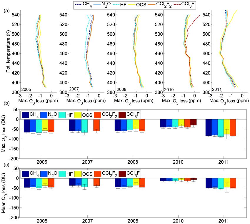
D. Griffin et al.: Ozone loss in the Arctic derived with ACE-FTS                                                                    581

processes that mix extra-vortex air into the polar vortex (e.g.       fitted linear correlation. The total error of ozone loss is de-
Plumb et al., 2000, 2003; Plumb, 2007), because it assumes            rived from the uncertainty of the passive ozone and the ACE-
that the polar vortex is isolated, which is not true for all years,   FTS v3.5 statistical fitting error for ozone, which are added
especially in the Arctic. On the other hand, some studies ob-         in quadrature.
serving Arctic ozone loss in the 1999–2000 winter (a winter
with an unusually strong polar vortex and thus little mixing)         3.2   Average vortex profile descent technique
have found that the mixing of mid-latitude air was not a sig-
nificant contributor to the observed changes (e.g. Richard et         Chemical ozone loss can be estimated by applying average
al., 2001; Ray et al., 2002). In our study, using the sPV cri-        vortex profile descent rates to the observed winter ozone pro-
teria described above, we attempt to limit the influence of           files. This determines the approximate vortex average pas-
mixing of extra-vortex air in our calculation of the early vor-       sive ozone profile that would be observed without chemical
tex reference function.                                               ozone depletion in spring for an isolated vortex. This method
    The tracer-tracer correlation method also neglects the de-        has previously been used by Manney et al. (2006) and Jin
scent of ozone or the tracer from high altitudes (middle and          et al. (2006), for example, to estimate Arctic ozone loss.
upper stratosphere and mesosphere) above 550 K that is not            The descent rates between January and March are derived
included in our calculation of the early vortex reference func-       at multiple potential temperature levels from the profile of a
tion. However, Salawitch et al. (2002) showed that the supply         long-lived tracer. These descent rates are then applied to the
of ozone-depleted air into the top of the vortex did not play         winter ozone profile to determine the passive ozone profile
a role in the subsequent evolution of the ozone-tracer rela-          in March. This method was originally utilized by estimat-
tion in the 1999–2000 Arctic winter (where the vortex was             ing the average vortex profile descent rate from N2 O profiles
strong). Mixing of air from top of the Arctic vortex (where           within the polar vortex, but many tracers can be used for this
mixing ratios are between 3 and 4 ppm Salawitch et al., 2002)         technique. Here, we have determined the chemical ozone de-
into the polar vortex could, however, underestimate the ozone         pletion by applying the profile descent rates, between Jan-
loss of the tracer-tracer method. In a case study for the spring      uary and March, from six long lived tracers: CH4 , HF, N2 O,
2003, Müller et al. (2007) showed that the mixing of meso-            CCl3 F, CCl2 F2 , and OCS. Note that this method only allows
spheric air is likely small and would not lead to an over-            for the estimation of one vortex averaged passive ozone pro-
estimation of the chemical ozone loss. Rex et al. (2002) state        file; all other methods applied in this study estimate a pas-
that the tracer-tracer correlation represents a lower limit of        sive ozone mixing ratio for each data point in March. Con-
the true ozone loss in the case of the 1999–2000 Arctic win-          sequently, this method does not consider any changes of the
ter (a year with a stable polar vortex).                              passive ozone levels that can occur throughout March. The
    With the tracer-tracer correlation method, a variety of           uncertainty of the passive ozone is estimated based on the
tracer gases can be used. A tracer is required to be long-            ±1σ standard deviation of the average vortex profile descent
lived (Plumb and Ko, 1992) and is thus not influenced by              (which is quite small for the average vortex profile descent
chemical processes over a polar season. Since ACE-FTS re-             technique). To obtain the total uncertainty, the statistical fit-
trieves profiles for a large number of different trace gases,         ting error of the ACE-FTS tracer measurements and the un-
we have tested six different tracers: CH4 , HF, N2 O, CCl3 F,         certainty of the passive ozone are added in quadrature. This
CCl2 F2 , and OCS. Figure 1 shows the O3 -tracer correlation          uncertainty estimate is based on statistical errors only and, as
between for these six tracers for the winter and spring of            such, underestimates the true uncertainty. It is difficult to esti-
2011. Displayed are the ACE-FTS measurements in January               mate the true uncertainty in this case because of the unknown
(black dots) and March (green dots) together with the esti-           effect of ozone resulting from mixing processes that are not
mated early vortex reference function (red solid line). There         considered for the average vortex profile descent technique.
is evidence of a large chemical ozone depletion in March,                An example for the average ACE-FTS N2 O profiles in-
since the March measurements are far from the estimated ref-          side the polar vortex between January (black line) and March
erence function. The ozone loss is estimated as the difference        (green line) 2011 is displayed in Fig. 2a. The strongest de-
between the measurements (green dots) and the early vortex            scent rates occur for high potential temperature levels (ap-
reference function (red line). For the estimation of the early        proximately −25 K/1.5 months), and a very slow descent was
vortex reference function, a fourth order polynomial was fit-         observed at 400 K (approximately −4 K/1.5 months). Fig-
ted for all of the different tracers. Previous studies have used      ure 2b displays the observed ozone in January (black dots)
a third- (e.g. Müller et al., 1997) or fourth-order polynomial        and March (green dots) of 2011. The passive ozone profile
fit (e.g. Tilmes et al., 2003; Müller et al., 2003; Tilmes et al.,    estimated from the N2 O average descent rate between Jan-
2004). We found that at least a third-order polynomial is re-         uary and March is shown as a blue line. The difference be-
quired, with little difference between third and fourth order;        tween the observed March ozone concentrations and passive
the fourth order is chosen to be consistent with the more re-         ozone profile is the estimate of the chemical ozone loss and
cent publications. The uncertainty of the calculated passive          is shown as red triangles. Similar figures using the remaining
ozone is estimated from the ±1σ standard deviation of the             tracers (except for CCl3 F, as not enough data were available

www.atmos-chem-phys.net/19/577/2019/                                                      Atmos. Chem. Phys., 19, 577–601, 2019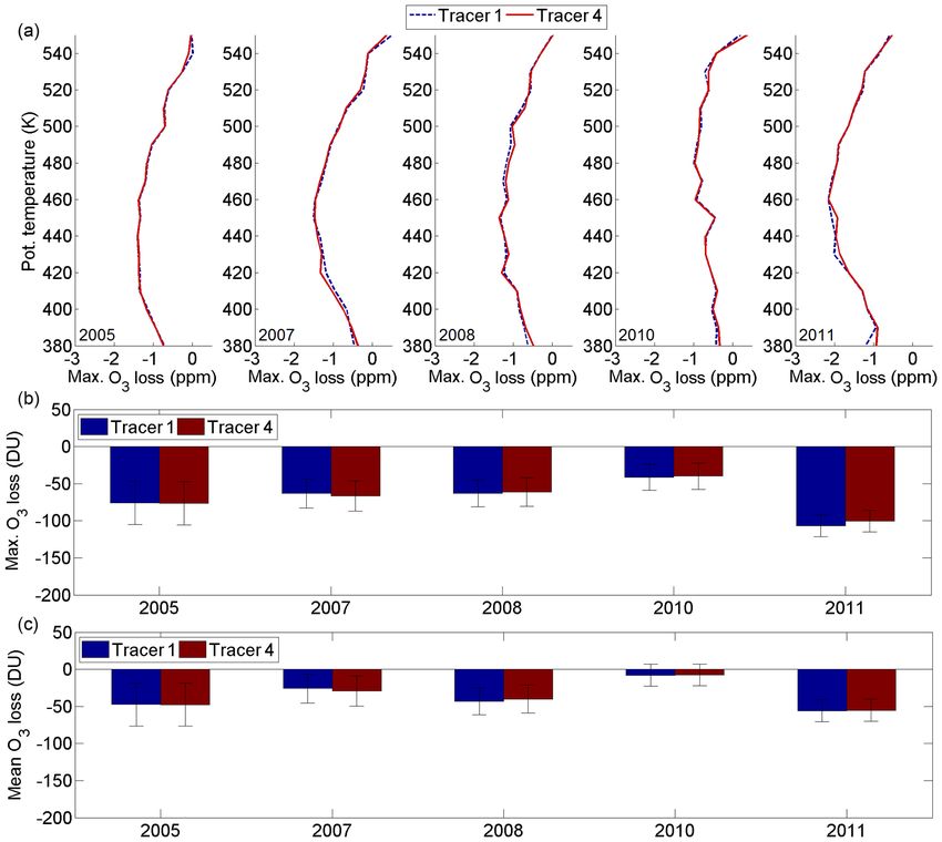
582                                                             D. Griffin et al.: Ozone loss in the Arctic derived with ACE-FTS

Figure 1. O3 -tracer correlation using ACE-FTS measurements inside the polar vortex in January (black dots) and March (green dots) 2011
using (a) CH4 , (b) HF, (c) N2 O, (d) CCl2 F2 , (e) CCl3 F, and (f) OCS as a tracer, in units of volume mixing ratios. The red line shows the
estimated early vortex reference function (see text for details) and the dashed black lines indicate the ±1σ standard deviation of the fit.

in 2011) can be found in the Supplement (Figs. S1–S4). The               easier to determine the ozone loss and reduces the impact of
plots are very similar for all of the tracers used in this study.        mixing, since mixing from the edge of the vortex would only
                                                                         result in “moving” the air parcels along this linear correla-
3.3   Artificial tracer method                                           tion line (Esler and Waugh, 2002). Initially such an artificial
                                                                         tracer method was used by Esler and Waugh (2002) to esti-
The amount of mixing of extra-vortex air into the Arctic polar           mate denitrification inside the Arctic polar vortex. However,
vortex varies widely depending on the dynamics of each win-              this same method can be applied for estimating the chem-
ter and spring (WMO, 2014). Neglecting mixing processes                  ical ozone loss, as was done by Jin et al. (2006). While it
from the edge of the polar vortex or the mixing of high al-              reduces the error from mixing of air near the vortex edge,
titude air (above the ozone maximum) can lead to an under-               this method, however, does not account for the mixing of
estimation of the chemical ozone loss (e.g. Rex et al., 2002;            extra-polar vortex air into the vortex. The artificial tracer, es-
Müller et al., 2005). One method that provides a correction              tablished from observations inside the polar vortex, does not
for both the mixing from the vortex edge and for the descent             follow the same linear correlation outside the polar vortex
is the artificial tracer method. This method was first proposed          (Jin et al., 2006).
by Esler and Waugh (2002) and uses a “tracer” created from a                Different combinations of tracers can be used to estimate
linear combination of several different trace gases that is lin-         an artificial tracer. Here, we have tested four different combi-
early correlated with ozone. This linear correlation makes it

Atmos. Chem. Phys., 19, 577–601, 2019                                                        www.atmos-chem-phys.net/19/577/2019/
D. Griffin et al.: Ozone loss in the Arctic derived with ACE-FTS 583
chemically depleted ozone between January and March. The
linear combination needed to obtain the artificial tracer is es-
timated for each year, since the trace gas concentrations and
the tracer–ozone correlation of these can vary from year-to-
year. It is assumed that the linear combination is constant on
a shorter time frame, e.g. within the polar vortex of one win-
ter (Esler and Waugh, 2002). This combination was found
to be similar (typically with constants on the same order of
magnitude, see Supplement Tables S1 and S2) in some years
between 2004 and 2013, but it was not the same for each
year. The uncertainty of the calculated passive ozone is es-
timated from the ±1σ standard deviation of the fitted linear
correlation. The total error of ozone loss is derived from the
uncertainty of the passive ozone and the ACE-FTS v3.5 sta-
tistical fitting error for ozone, which are added in quadrature.
An example of the artificial tracer correlation for all four
artificial tracers is shown in Fig. 3. The data shown are mix-
ing ratios inside the polar vortex during January (black dots)
and March (green dots) 2011. While Tracer 1, Tracer 2, and
Tracer 4 show a linear correlation with ozone and a small
standard deviation, Tracer 3 is not quite linearly correlated
and consequently has a larger uncertainty. There is strong
evidence in these figures of the chemical ozone depletion in
2011, since the ozone levels in March are very low compared
to January and are not linearly correlated with the artificial
tracers. The passive ozone is estimated from the linear fit
by assuming that without any chemical ozone depletion, the
Figure 2. (a) shows the monthly average N2 O profiles observed by
ozone levels should still follow this correlation in March. The
ACE-FTS inside the polar vortex in January (black line) and March
linear combinations used to estimate the artificial tracers for
(green line) 2011 together with the respective standard deviations
(shown as dashed lines). (b) displays the observed ACE-FTS ozone the 2011 dataset, are
in January (black dots) and March (green dots) 2011, the passive
ozone (blue line) for March 2011, estimated from the average vortex [Tracer1]ppb = 9.34 × 10⁻⁴ [CH4 ]ppb − 7.45 × 10⁻⁴ [N2 O]ppb
profile descent from N2 O, and the ozone loss (red triangles; the − 3.41 × 10⁻³ [CCl2 F2 ]ppt − 9.46
difference between observed and average passive ozone in March).
× 10−3 [CCl3 F]ppt + 2.86, (1)
−3 −2
[Tracer2]ppb = 4.86 × 10 [CH4 ]ppb − 1.63 × 10 [N2 O]ppb
nations that were employed by Esler and Waugh (2002) and
+ 1.43 × 10⁻³ [CFC-113]ppt − 1.52
Jin et al. (2006). These tracers include a combination of
× 10−2 [CCl3 F]ppt − 0.175, (2)
1. N2 O, CH4 , CCl3 F, and CCl2 F2 (Esler and Waugh, −4 −3
[Tracer3]ppb = 3.20 × 10 [CH4 ]ppb − 1.73 × 10 [N2 O]ppb
2002);
− 5.59 × 10⁻³ [CCl2 F2 ]ppt + 3.77, (3)
2. N2 O, CH4 , CCl3 F, and CFC-113 (Esler and Waugh, −4 −4
[Tracer4]ppb = 2.22 × 10 [CH4 ]ppb − 5.03 × 10 [N2 O]ppb
2002);
− 3.91 × 10⁻³ [OCS]ppt − 6.05
3. N2 O, CH4 , and CCl2 F2 (Esler and Waugh, 2002); × 10−3 [CCl2 F2 ]ppt + 3.15. (4)
4. N2 O, CH4 , OCS, and CCl3 F (Jin et al., 2006).
Since Tracer 3 is not highly linearly correlated with ozone
These artificial tracers will be referred to, in this paper, as (R = 0.9, the other tracers have R ≥ 0.95; see Tables S1 and
Tracer 1, Tracer 2, Tracer 3, and Tracer 4, respectively. To S2 in the Supplement) and has a standard deviation of ap-
estimate the artificial tracer that is linearly correlated with proximately 10 % (see Fig. 3), this tracer has been elimi-
ozone, ACE-FTS measurements inside the polar vortex in nated from further analysis, as it seems unsuitable for deter-
January are employed. The correlation is then used to esti- mining the passive ozone accurately. Tracer 2 contains CFC-
mate the passive ozone levels that would be observed without 113, which has limited coverage at higher altitudes due to a
chemical ozone depletion in March. The difference between processing issue. As such, limited measurements are avail-
the observed ozone and estimated passive ozone equals the able to determine the passive ozone with this artificial tracer.
www.atmos-chem-phys.net/19/577/2019/ Atmos. Chem. Phys., 19, 577–601, 2019584 D. Griffin et al.: Ozone loss in the Arctic derived with ACE-FTS
Figure 3. Artificial tracer correlation technique using ACE-FTS measurements inside the polar vortex in January (black dots) and March
(green dots) 2011 using (a) Tracer 1, (b) Tracer 2, (c) Tracer 3, and (d) Tracer 4. The fitted correlations are shown as red lines, and the black
lines indicate the ±1σ standard deviation of the fit. See text for further details on the artificial tracers.
Consequently, Tracer 2 is not a suitable tracer to use with 3.4.1 Passive subtraction with ATLAS
the ACE-FTS v3.5 dataset. For further analysis only Tracer 1
and Tracer 4 were considered for determining the ozone de-
The ATLAS model was specifically developed to assess
pletion.
stratospheric chemistry, transport, and mixing. Passive ozone
and the ozone that responds to both heterogeneous and ho-
3.4 Passive subtraction using CTMs mogeneous chemistry can be estimated with this model;
however, in this study, only the passive ozone is used and
In addition to approaches that only use the ACE-FTS dataset, compared to the ACE-FTS measurements to obtain the
the chemical ozone depletion was estimated by employing chemical ozone depletion. This model was previously used
passive ozone from CTMs. The passive ozone from two dif- to estimate stratospheric ozone within the polar vortex (e.g.
ferent models, the Lagrangian ATLAS (Alfred Wegener In- Adams et al., 2013; Wohltmann et al., 2013), and valida-
stitute Lagrangian chemistry and transport system; Wohlt- tion comparisons with measurements and other models have
mann and Rex, 2009; Wohltmann et al., 2010) and the Eule- shown good agreement (Wohltmann and Rex, 2009; Wohlt-
rian SLIMCAT (Chipperfield et al., 2006) models, has been mann et al., 2010, 2013, 2017). For the model run presented
used to investigate the chemical ozone depletion in March in this study, the passive tracer was initialized each year on 1
2004–2013. Within these models, ozone can be treated as January with Aura MLS (Waters et al., 2006) v3.3/3.4 ozone
a passive tracer that is not influenced by chemical deple- measurements. The ACE-FTS dataset cannot be used for this,
tion processes, and only dynamics are applied to the mod- since its daily latitude coverage is not sufficient for the initial-
elled ozone concentrations. The passive subtraction methods ization of the model. However, relative differences between
using CTMs account for mixing of extra-polar vortex air; Aura MLS and ACE-FTS ozone concentrations are small, be-
however, it is difficult to determine how well these mixing tween 2 and 5 % in the stratosphere (Sheese et al., 2016). The
processes are represented within those models. Both models passive ozone output has a horizontal resolution of 150 km.
used in this study are driven by driven by the European Cen- The vertical coordinate is potential temperature (∼350 to
tre for Medium-range Weather Forecasts Reanalysis Interim 1900 K). The vertical resolution of the model changes de-
(ECMWF ERA-Interim) meteorological reanalysis (Dee et pending on altitude and is typically between 10 and 40 K at
al., 2011). In both models, ozone chemistry can be included altitudes between 350 and 550 K. Passive ozone concentra-
by employing appropriate chemical reactions. tions are saved every 12 h at 00:00 and 12:00 UTC.
Atmos. Chem. Phys., 19, 577–601, 2019 www.atmos-chem-phys.net/19/577/2019/D. Griffin et al.: Ozone loss in the Arctic derived with ACE-FTS 585
Since ATLAS is a Lagrangian transport model, the loca-
tions of the model output change and are most likely not co-
incident with the location of the ACE-FTS measurements.
To obtain the passive ozone concentration at the location
of each 1 km tangent altitude for each ACE-FTS measure-
ment, back or forward trajectories are utilized at individual
altitudes to obtain the ACE-FTS measurement location or
“end point” at the time of the ATLAS output. Since pas-
sive ozone amounts are obtained from ATLAS every 12 h,
the back or forward trajectories are estimated for a maxi-
mum of 6 h. These forward and back trajectories were cal-
culated with HYSPLIT (Hybrid Single-Particle Lagrangian
Integrated Trajectory; Draxler and Hess, 2004), using the
NCEP (National Centers for Environmental Prediction) re-
analysis (Kalnay et al., 1996) for the meteorological input.
Note that the time period of the back and forward trajectories
is relatively short (a maximum of 6 h); therefore differences
in the meteorological input used to drive the CTM and those
used for the trajectory calculations are small compared to the
total uncertainty. The ATLAS data points that are at the same
potential temperature levels (within ATLAS vertical resolu-
tion) as the end point of the ACE-FTS measurement are then
triangulated. If the three closest ATLAS points that surround
the end point of the trajectory are inside the polar vortex, they
are interpolated to this position using a barycentric method.
The interpolation is only done horizontally; we did not apply
Figure 4. (a) shows a comparison between the ATLAS passive
interpolation in the vertical direction but instead chose only ozone and ACE-FTS ozone dataset inside the polar vortex for Jan-
ATLAS points that were at the same potential temperature uary 2011. The black dots represent the individual data points and
levels as the ACE-FTS observations, within the resolution of the red line indicates the line of best fit. For easy comparison, the
ATLAS. one-to-one line is shown as a black dashed line. (b) shows ATLAS
The passive ozone mixing ratios are compared to the ACE- passive O3 (blue dots), ACE-FTS measurements (green dots), and
FTS measurements in January and March. The difference the ozone loss (red triangles; the difference between observed and
between the March measurements and the passive ozone is average passive ozone) for March 2011.
considered the chemical ozone loss. The difference between
the ACE-FTS dataset and ATLAS for January is used to es-
timate an uncertainty of the modelled ozone. To determine This difference between the ATLAS passive and ACE-FTS
the uncertainty of the model results, the relative differences measured ozone is likely due to the difference between the
between ACE-FTS measurements and the ATLAS passive Aura MLS and ACE-FTS datasets that is of the same order
ozone for January are calculated as [ACE-FTS−ATLAS] / of magnitude. However, some of this difference could also
[0.5× (ACE − FTS + ATLAS)]. These vary between 0.7 and be due to early ozone depletion in January, as was seen by
5.2 %, depending on the individual year. Note that these un- Manney et al. (2015). The ACE-FTS measurements (green
certainty estimates may include the effects of January ozone dots) and ATLAS passive ozone (blue dots) for March 2011
loss, which cannot be determined from these datasets. For are displayed in Fig. 4b. The difference between the ATLAS
the total uncertainty of the chemical ozone loss, the statisti- and ACE-FTS ozone concentrations are displayed as red tri-
cal fitting error from ACE-FTS v3.5 O3 measurements and angles and indicate chemical ozone loss.
the mean difference of ACE-FTS measurements and ATLAS
passive ozone in January are added in quadrature. Note that 3.4.2 Passive subtraction with SLIMCAT
the uncertainty estimated here is a lower bound on the actual
uncertainty, since it does not consider the accumulated uncer- In addition to ATLAS, we have also used the SLIMCAT off-
tainties in model transport since the initialization in January line 3-D CTM to investigate Arctic ozone loss. This model
(e.g. caused by deficiencies in the ERA-Interim). has been widely used to study the stratospheric ozone abun-
An example of the comparisons for January 2011 is dance and chemical ozone depletion (e.g. Feng et al., 2007;
shown in Fig. 4a. ATLAS passive and ACE-FTS measured Sinnhuber et al., 2000; Singleton et al., 2005, 2007; Adams
ozone are in good agreement. The difference is, on average, et al., 2012; Lindenmaier et al., 2012; Dhomse et al., 2013;
−5.2 ± 0.7 %, with a high correlation coefficient (R = 0.94). Chipperfield et al., 2015). A detailed description of the model
www.atmos-chem-phys.net/19/577/2019/ Atmos. Chem. Phys., 19, 577–601, 2019586 D. Griffin et al.: Ozone loss in the Arctic derived with ACE-FTS can be found in Chipperfield et al. (2006), and recent up- dates are described in Dhomse et al. (2013) and Chipperfield et al. (2015). SLIMCAT uses an Eulerian grid that extends from pole to pole. It contains a detailed stratospheric chem- istry scheme including all processes that are related to po- lar ozone depletion (Chipperfield et al., 2006; Dhomse et al., 2013, and references therein). As such, passive ozone and ozone that responds to ozone chemistry are modelled. The model was also forced by ERA-Interim meteorological reanalysis (Dee et al., 2011). The passive ozone from the SLIMCAT model run was reset on 1 January for each year to the values of the model chemical ozone field at that time. The model simulation used here has a horizontal resolution of 2.8◦ ×2.8◦ , and the vertical coordinate is defined on hybrid σ -pressure vertical levels between the surface and approx- imately 60 km on 32 layers. The simulation was initialized in 1979 (using output from a 2-D model) and constrained by specified global mean surface observations of long-lived source gases. SLIMCAT therefore simulates ozone and all other stratospheric trace gases for all years in this study in a single long-term simulation. The model was sampled at the locations of the 30 km tangent altitude of the ACE-FTS oc- cultations providing profiles of the passive ozone and ozone that responds to ozone chemistry corresponding to each mea- surement. Although the geolocations of the ACE-FTS mea- surements change with altitude, the location of the measure- ments at the altitudes of interest (approximately 15–25 km) are within an approximately 0.5◦ great circle of the loca- tion of the 30 km tangent altitude and are therefore within the model resolution. Therefore, the measurements and the mod- elled ozone fields can be directly compared without further processing. The ozone loss was estimated from the difference between the modelled passive ozone and the observed ozone inside the polar vortex in March. Additionally, the ozone loss has also been estimated by solely using both the mod- elled ozone that responds to ozone chemistry and the pas- sive ozone from the model (referred to as “SLIMCAT only”). This helps to estimate the uncertainty of the modelled ozone (that includes ozone chemistry) by comparing it to the mea- Figure 5. (a) shows a comparison between the SLIMCAT ozone surements and can indicate potential ozone loss in January and ACE-FTS ozone dataset inside the polar vortex for January by comparing the passive ozone and ozone (that includes (black dots) and March (green dots) 2011, with the combined re- ozone chemistry). To estimate the uncertainty of the model gression fit for January and March shown as a red line. (b) and (c) results, the relative differences between ACE-FTS measure- show the comparison between the SLIMCAT ozone (passive ozone ments and the SLIMCAT ozone for January and March – SLIMCAT – shown as blue dots, and ozone with “active” chem- are calculated as [ACE-FTS − SLIMCAT] / [0.5×(ACE- istry – Act. SLIMCAT – as cyan triangles) and measurements (green FTS + SLIMCAT)]. The ACE-FTS ozone measurements and dots) for January 2011 and March 2011, respectively. The ozone the modelled ozone agree very well, with mean relative dif- loss is displayed as red triangles and defined as the difference be- ferences between 0.8 and 4.8 % (and R ≈ 0.95), depending tween the measurements and the modelled passive ozone. on the specific year. The total uncertainty of the ozone loss was estimated in a similar way as was done for the ATLAS analysis (see Sect. 3.4.1); the ACE-FTS ozone measurement uncertainties in model transport (e.g. caused by deficiencies fitting error and the mean relative difference between ACE- in the ERA-Interim). FTS and SLIMCAT ozone were added in quadrature. Note An example of the comparison for January and March that the uncertainty estimated here is a lower bound on the 2011 is shown in Fig. 5a. The measurements and the model actual uncertainty, since it does not consider the accumulated ozone are in good agreement with a mean difference of Atmos. Chem. Phys., 19, 577–601, 2019 www.atmos-chem-phys.net/19/577/2019/
D. Griffin et al.: Ozone loss in the Arctic derived with ACE-FTS                                                                          587

Figure 6. The ozone loss estimates are shown using the tracer-tracer correlation technique. Six different tracers have been employed for this
method: CH4 (blue), N2 O (light blue), HF (cyan), OCS (yellow), CCl2 F2 (orange), and CCl3 F (dark red). The maximum ozone loss profile
(in ppmv) is shown in (a). For clarity, the uncertainties of the estimated ozone loss profiles have been removed. The integrated ozone loss (in
DU) between 380–550 K is shown in (b) and (c) for the maximum and mean loss in March, respectively.

3.9±0.8 %, and the correlation is high, with a correlation co-            4.1   Impact of the choice of tracer
efficient R = 0.95. This result confirms that the model simu-
lates the measured ozone quite well. In Fig. 5b and c, ACE-
FTS measurements (green dots), SLIMCAT ozone (cyan tri-                   For the tracer-tracer correlation method and the average vor-
angles) and SLIMCAT passive ozone (blue dots) are dis-                    tex profile descent technique, six long-lived tracers (CH4 ,
played for January and March 2011, respectively. The ozone                N2 O, HF, OCS, CCl3 F, and CCl2 F2 ) have been used to esti-
loss (red triangles) is obtained from the observed and mod-               mate the chemical ozone depletion in the Arctic polar vortex
elled passive ozone, and indicates the chemical ozone loss.               in March with respect to January. These results are shown
Figure 5b confirms that little ozone depletion was observed               in Figs. 6 and 7, respectively. Two different combinations
in January 2011, as the differences between the measured and              of tracers have been investigated to create an artificial tracer
modelled passive ozone are on average around 0.1 ppmv. The                that is linearly correlated with ozone, and these results are
results of the estimated ozone loss are discussed in Sect. 4.             displayed in Fig. 8. Panel (a) of Figs. 6–8 shows the mix-
                                                                          ing ratio loss profile of the maximum chemical ozone loss
                                                                          between 380 and 550 K in March 2005, 2007, 2008, 2010,
4   Annual intercomparison and interpretation of Arctic
                                                                          and 2011. The partial-column ozone loss presented here is
    ozone loss estimates
                                                                          estimated from the mixing ratio losses using the mean alti-
In this section, the impact of the different tracers and the dif-         tudes of the DMP’s potential temperature profile, between
ferent methods on the estimated ozone loss is discussed for               380 K and 550 K, and the ACE-FTS densities at the given
the 5 years where no SSW event occurred. The mixing ratio                 altitude level. This interpolation to altitude levels was nec-
profile and partial-column (380–550 K) ozone depletion are                essary for the estimation of the integrated partial columns
compared, and the differences are discussed.                              (Nathaniel Livesey, personal communication, 2016). Panels
                                                                          (b) and (c) of Figs. 6–8 show the maximum and mean partial-
                                                                          column ozone loss, respectively. The error bars displayed in
                                                                          panels (b) and (c) of Figs. 6–8 indicate the uncertainty of the
                                                                          maximum and mean column ozone loss estimates that are

www.atmos-chem-phys.net/19/577/2019/                                                           Atmos. Chem. Phys., 19, 577–601, 2019
588 D. Griffin et al.: Ozone loss in the Arctic derived with ACE-FTS Figure 7. Same as Fig. 6, but for the average vortex profile descent technique. derived from maximum and mean ozone loss VMR uncer- timates are different for different tracers, the partial-column tainties, respectively, as calculated in Sect. 3. losses (maximum and mean) are not significantly different For the tracer-tracer correlation method (Fig. 6), the results and agree within the estimated uncertainties. for all six tracers are similar for the partial-column ozone. Both OCS and CCl3 F results show a smaller ozone loss However, there are differences apparent in the profile of the (∼ 0.5–1 ppmv) above approximately 500 K compared to the estimated ozone loss for each tracer, especially for high and other tracers in all years. For most years, the ozone loss pro- low altitudes. The estimated uncertainties of the ozone loss files computed with CH4 , N2 O, HF, and CCl2 F2 agree well profile are ∼0.2–0.6 ppmv, or approximately ∼ 10–20 % of and within the estimated uncertainties for the entire profile. the estimated ozone loss, and the results from all tracers The largest discrepancies between the tracers occur in 2005, agree within the uncertainties between approximately 460– when the vortex was relatively weak and influenced by mix- 500 K for all years, with the exception of 2005. Both mixing ing. Also, in 2007, the estimated loss is larger when HF is and strong ozone loss was apparent in the winter of 2004– used as a tracer, and it does not follow the ozone loss profile 2005 (e.g. Manney et al., 2006) and is consequently a good as estimated with other tracers. For the partial-column losses, year to test the agreement between the different tracers. As all tracers agree within the estimated uncertainties. However, shown in Fig. 6a, the profiles of the different tracers do not these uncertainties are quite large, between approximately 20 agree well in March 2005. This indicates the shortcomings and 40 DU, and represent roughly 40–60 % of the estimated of the tracer-tracer correlation method, even in cases where ozone loss. The estimated profile and partial-column ozone only inner core vortex measurements were used for estimat- loss is consistently smaller (∼ 10 DU) if OCS or CCl3 F is ing the ozone loss. These results are consistent with previ- used as the tracer. In the ACE-FTS v3.5 dataset many CCl3 F ous studies (e.g. Michelsen et al., 1998; Plumb et al., 2000, retrievals fail, especially in higher altitudes. Typically only 2003; Plumb, 2007) that have shown that tracer-tracer corre- one quarter to half as many profiles are available each year lations are not expected to be accurate for estimating Arctic compared to the other tracers. Due to this limited coverage, ozone loss. However, in this study, though the profile loss es- the column ozone loss could only be estimated with CCl3 F in Atmos. Chem. Phys., 19, 577–601, 2019 www.atmos-chem-phys.net/19/577/2019/
D. Griffin et al.: Ozone loss in the Arctic derived with ACE-FTS                                                                             589

Figure 8. Similar to Fig. 6, but for the artificial tracer correlation method. Tracer 1 (N2 O, CH4 , CCl2 F2 , and CCl3 F) in dark blue and Tracer
4 (N2 O, CH4 , OCS, and CCl3 F) in dark red. Details about the composition of the four tracers are provided in the text.

2011. It should be noted that OCS has a significantly shorter              polar vortex rather than descent is estimated (for all calcu-
stratospheric lifetime that is approximately 2 years (Montzka              lated descent rates, see Tables S3–S8 in the Supplement).
et al., 2007; Dhomse et al., 2014), whereas all other trac-                In 2007–2008 and 2010–2011, when CH4 , N2 O, HF, and
ers have lifetimes of over 50 years (Hoffmann et al., 2014;                CCl2 F2 estimate a large descent of approximately 20–35 K
Brown et al., 2013). As OCS is not as stable as all other trac-            over 1.5 months (between approximately 450–550 K; see Ta-
ers, this could negatively impact the ozone loss estimation                bles S3–S8 in the Supplement), OCS only estimates half as
using OCS.                                                                 much. The reason for this could be the limited precision of
   Using these six different tracers to estimate the average               the ACE-FTS OCS retrievals that have retrieval fitting errors
vortex descent rate (Fig. 7) leads to very similar results                 of around 10 %, almost 10 times higher than for other species
for most tracers, except for OCS. The uncertainties for this               (e.g. O3 and N2 O). As shown in Fig. 7a, the mixing ratio loss
method are ∼0.02–0.1 ppmv, or ∼1–10 %. These are smaller                   profile is very similar with all different tracers, with the ex-
than the ones estimated for the tracer-tracer method due to                ception of HF in 2007, where a larger chemical ozone de-
the small standard deviation of the average vortex descent                 pletion is estimated. This large discrepancy is also seen in
profile. Note that this does not represent the true uncertainty            2007 for the tracer-tracer correlation method. For this win-
and represents a statistical uncertainty. The true uncertainty             ter, the descent rates using HF are almost twice as large as
is likely much higher, since only one passive ozone profile                those derived from the other tracers; for all other years HF
for each March is applied (and, therefore, the same amount                 provides descent rates that are similar to the other tracers.
of ozone at each potential temperature level). The profile loss            Due to the large estimated uncertainties of the integrated loss
estimated for these different tracers looks similar for most               (∼ 2.4–6.5 DU), the estimated partial-column ozone loss for
years, with the exemption of OCS in 2005, 2008, and 2011,                  each year agrees for all different tracers within the estimated
and CCl3 F in 2010. During the winters of 2004–2005, 2006–                 uncertainties. Only in 2010 could the partial-column ozone
2007, and 2009–2010, when using OCS, an ascent inside the                  depletion (between 380–550 K) be estimated using CCl3 F

www.atmos-chem-phys.net/19/577/2019/                                                             Atmos. Chem. Phys., 19, 577–601, 2019
You can also read