MCRALI: A MONTE CARLO HIGH-SPECTRAL-RESOLUTION LIDAR AND DOPPLER RADAR SIMULATOR FOR THREE-DIMENSIONAL CLOUDY ATMOSPHERE REMOTE SENSING - RECENT
←
→
Page content transcription
If your browser does not render page correctly, please read the page content below
Atmos. Meas. Tech., 14, 199–221, 2021
https://doi.org/10.5194/amt-14-199-2021
© Author(s) 2021. This work is distributed under
the Creative Commons Attribution 4.0 License.

McRALI: a Monte Carlo high-spectral-resolution lidar and Doppler
radar simulator for three-dimensional cloudy
atmosphere remote sensing
Frédéric Szczap1 , Alaa Alkasem1 , Guillaume Mioche1,2 , Valery Shcherbakov1,2 , Céline Cornet3 , Julien Delanoë4 ,
Yahya Gour1,5 , Olivier Jourdan1 , Sandra Banson1 , and Edouard Bray1
1 Université Clermont Auvergne, CNRS, UMR 6016, Laboratoire de Météorologie Physique (LaMP), 63178 Aubière, France
2 Université Clermont Auvergne, Institut Universitaire de Technologie d’Allier, 03100 Montluçon, France
3 Université Lille, CNRS, UMR 8518, Laboratoire d’Optique Atmosphérique (LOA), 59000 Lille, France
4 Université de Versailles Saint-Quentin-en-Yvelines, Université Paris-Saclay, Sorbonne Université, CNRS, Laboratoire

Atmosphère, Milieu, Observations Spatiales (LATMOS), Institut Pierre Simon Laplace (IPSL), Guyancourt, France
5 Université Clermont Auvergne, Institut Universitaire de Technologie d’Allier, 03200 Vichy, France

Correspondence: Frédéric Szczap (szczap@opgc.univ-bpclermont.fr)

Received: 16 June 2020 – Discussion started: 8 July 2020
Revised: 20 October 2020 – Accepted: 18 November 2020 – Published: 12 January 2021

Abstract. The aim of this paper is to present the Monte Carlo      1   Introduction
code McRALI that provides simulations under multiple-
scattering regimes of polarized high-spectral-resolution           Spaceborne atmospheric lidar (light detection and ranging)
(HSR) lidar and Doppler radar observations for a three-            and radar (radio detection and ranging) are suitable tools to
dimensional (3D) cloudy atmosphere. The effects of nonuni-         investigate vertical properties of clouds on a global scale.
form beam filling (NUBF) on HSR lidar and Doppler radar            Over the last decade, the Cloud–Aerosol Lidar and Infrared
signals related to the EarthCARE mission are investigated          Pathfinder Satellite Observations (CALIPSO) (Winker et al.,
with the help of an academic 3D box cloud characterized            2010) and the Cloud Satellite (CloudSat) (Stephens et al.,
by a single isolated jump in cloud optical depth, assum-           2008) have improved our understanding of the spatial dis-
ing vertically constant wind velocity. Regarding Doppler           tribution of microphysical and optical properties of clouds
radar signals, it is confirmed that NUBF induces a severe          and aerosols (Stephens et al., 2018). However, clouds re-
bias in velocity estimates. The correlation of the NUBF            main the largest source of uncertainty in climate projec-
bias of Doppler velocity with the horizontal gradient of           tions (Boucher et al., 2014; Dufresnes and Bony, 2008). Like
reflectivity shows a correlation coefficient value around          clouds, aerosols are another large source of uncertainty in cli-
0.15 m s−1 (dBZ km−1 )−1 , close to that given in the scien-       mate models (both direct and indirect radiative forcing) (see,
tific literature. Regarding HSR lidar signals, we confirm that     e.g., Hilsenrath and Ward, 2017, and references therein).
multiple-scattering processes are not negligible. We show          Future missions are planned to pursue those observations.
that NUBF effects on molecular, particulate, and total atten-      For example, the Earth Clouds, Aerosol and Radiation Ex-
uated backscatter are mainly due to unresolved variability of      plorer (EarthCARE) (Illingworth et al., 2015) is scheduled
cloud inside the receiver field of view and, to a lesser extent,   for 2022, which will deploy the combination of a high-
to the horizontal photon transport. This finding gives some        resolution-spectral (HSR) lidar and a Doppler radar for the
insight into the reliability of lidar signal modeling using in-    first time in space. More recently, following the Atmospheric
dependent column approximation (ICA).                              Dynamics Mission ADM-Aeolus (ESA report, 2016) by the
                                                                   European Space Agency (ESA), an atmospheric dynamics
                                                                   observation satellite was placed in orbit in August 2018,
                                                                   which deployed the first space Doppler lidar. The Atmo-

Published by Copernicus Publications on behalf of the European Geosciences Union.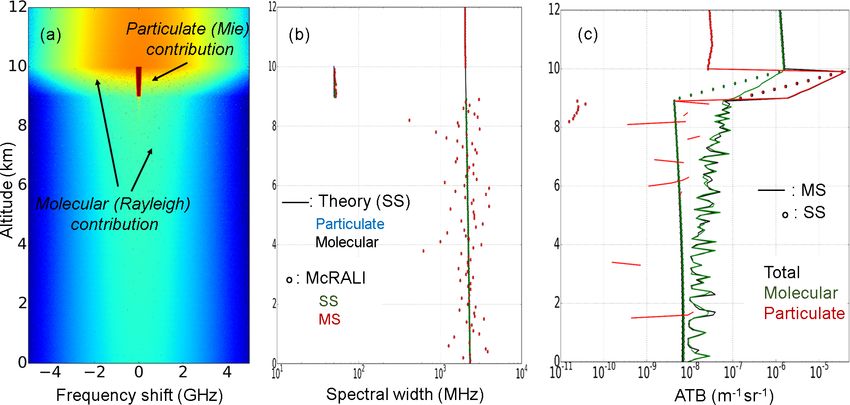
200 F. Szczap et al.: McRALI: a Monte Carlo high-spectral-resolution simulator
spheric LAser Doppler INstrument (ALADIN) of the ADM- nonuniform beam-filling (NUBF) scenarios (Battaglia and
Aeolus provides spectrally resolved data. Indeed, the Mie Tanelli, 2011). Note that DOMUS is not a part of ECSIM.
receiver is a Fizeau spectrometer combined with a charge- The McRALI simulators (Monte Carlo modeling of
coupled detector that measures the spectrum of the return RAdar and LIdar signals) developed at the Laboratoire de
around the emitted laser wavelength using 16 different fre- Météorologie Physique (LaMP) are based on 3DMcPOLID
quency bins (Reitebuch et al., 2018; Stoffelen et al., 2005). (3D Monte Carlo simulator of POLarized LIDar signals), an
The ATmospheric LIDar (ATLID) signals of the EarthCARE MC code dedicated to simulating polarized active sensor sig-
mission will be optically filtered in such a way that the atmo- nals from atmospheric compounds in single- and/or multiple-
spheric Mie and Rayleigh scattering contributions are sepa- scattering conditions (Alkasem et al., 2017). As their core
rated and independently measured (Pereira do Carmo et al., they use the three-dimensional polarized Monte Carlo atmo-
2019). The radar echoes of the Cloud Profiling Radar (CPR) spheric radiative transfer model (3DMCPOL; Cornet et al.,
of the EarthCARE mission will be input to autocovariance 2010). Like 3DMCPOL, they use the local estimate method
analysis by means of the pulse-pair processing technique for (Marchuk et al., 1980; Evans and Marshak, 2005) to re-
the estimation of the Doppler properties (Kollias et al., 2014, duce the noise level and take into account the polarization
2018; Zrnić, 1977). Note, however, that ATLID and CPR state of light. Photons are followed step by step through the
will not provide spectrally resolved data. The CPR will pro- cloudy atmosphere. At each interaction, the contribution to
vide information on convective motions, wind profiles, and the detector is computed according to the scattering matrix
fall speeds (Illingworth et al., 2015). The ATLID will per- and the field of view (FOV) of the detector. Variance reduc-
form measurements of the extinction coefficient and lidar ra- tion techniques proposed by Buras and Mayer (2011) can
tio (ESA, 2016; Illingworth et al., 2015). be employed for the purpose of reducing noise due to the
Lidar and/or radar simulators are steadily advancing, strong forward scattering peak and consequently increasing
hence allowing us to explore direct and inverse problems in the computational efficiency. All simulations in this work
a cost-effective way. In this Introduction, published works were done without application of the variance reduction tech-
restricted to the case when multiple scattering was taken niques.
into account are briefly discussed. Fruitful findings, mostly The objective of this work is to describe the latest evolu-
on lidar returns from clouds, were obtained by the MUS- tion of McRALI, which provides the means to simulate high-
CLE (MUltiple SCattering in Lidar Experiments) commu- spectral-resolution (HSR) lidar and Doppler radar signals.
nity in the 1990s. A review of the participating models The organization of this paper is as follows. In Sect. 2, we
can be found in the work by Bissonnette et al. (1995). A explain in detail the methodology used in McRALI to model
Monte Carlo (MC) model was used by Miller and Stephens spectral properties of lidar or radar data. Two illustrative ap-
(1999) to study the specific roles of cloud optical proper- plications (i.e., ATLID lidar and CPR radar of the Earth-
ties and instrument geometries in determining the magni- CARE mission) of the developed simulator are presented. In
tude of lidar pulse stretching. Several models, which take Sect. 3 we briefly investigate errors induced by NUBF to the
into consideration Stokes parameters, were developed in the EarthCARE lidar and radar measurements with the help of
2000s (Hu et al., 2001; Noel et al., 2002; Ishimoto and Ma- the academic 3D box cloud. This work is unique in that the
suda, 2002; Battaglia et al., 2006). Fast approximate lidar results can be obtained only if the simulator is a fully 3D
and radar multiple-scattering models (Chaikovskaya, 2008; Monte Carlo forward model. Conclusions and discussions
Hogan, 2008; Hogan and Battaglia, 2008; Sato et al., 2019) are presented in Sect. 4.
provide the possibility, for example, to explain certain im-
portant characteristics of dual-wavelength reflectivity pro-
files (Battaglia et al., 2015), although the codes are inher- 2 Modeling of HSR lidar and Doppler radar signals
ently one-dimensional. In addition, a comprehensive review with McRALI
of multiple scattering in radar systems can be found in the
work by Battaglia et al. (2010). The basic principles of Monte 2.1 General principles for the computation of
Carlo models, which consider the Doppler effect and spectral frequency-resolved signal
properties of received signals, were developed in the 1990s
for the needs of laser Doppler flowmetry (see, e.g., de Mul et A basic lidar or radar equation can be written as (Weitkamp,
al., 1995, and references therein). As for lidar and radar mea- 2005; Battaglia et al., 2010)
surements, we can refer to the EarthCARE simulator (EC-
Zr
SIM) that is a modular multi-sensor simulation framework, K (r)
p (r) = 2 β (r) exp −2 σext r 0 dr 0 ,
wherein a fully 3D Monte Carlo forward model can calculate (1)
r
the spectral polarization state of ATLID lidar signals (Dono- 0
van et al., 2008; Donovan et al., 2015). A radar Doppler
multiple-scattering (DOMUS) simulator can be run in a full where p is the power on the detector from range r, K is the
3D configuration and allows a comprehensive treatment of instrument function, σext (in m−1 ) is the extinction, and β (in
Atmos. Meas. Tech., 14, 199–221, 2021 https://doi.org/10.5194/amt-14-199-2021
F. Szczap et al.: McRALI: a Monte Carlo high-spectral-resolution simulator                                                            201

m−1 sr−1 ) is the backscattering coefficient defined as                 for each of the computed Stokes parameters, without consid-
                                                                        ering the Doppler spectrum folding depending on the mea-
β = P (π ) σs ,                                                  (2)    surement technology (step 2 in Fig. 1). The generic name
                                                                        McRALI-FR will be used for our frequency-resolved simu-
where P (π ) (in sr−1 ) is the scattering phase function in the         lators.
backward direction and σs (in m−1 ) is the scattering coeffi-              The simulation conditions (step 1 in Fig. 1) consists of set-
cient. Whereas the lidar community uses the backscattering              ting the 3D optical and dynamical properties of the cloudy
coefficient β, the radar community prefers to use the reflec-           atmosphere, the surface, and main characteristics of the in-
tivity Z related to β as                                                strument (currently monostatic high-spectral-resolution lidar
           4                                                          or a Doppler radar), which are its spatial position, its veloc-
        4  λ                                                            ity, the viewing direction, the frequency and the polarization
Z=      2
               β,                                                (3)
   |Kw |   π                                                            state of the emitted radiation, and the shape of the emitter
                                                                        and the receiver. If at least one of those parameters varies,
where |Kw |2 is a dielectric factor usually assumed for liq-            the simulation has to be carried out once more even when 3D
uid water and λ is the wavelength. Due to its large dy-                 cloudy atmosphere properties remain unchanged. Computa-
namic range, the radar reflectivity factor (usually expressed           tions are carried out and profiles of S(r, f ) are stored in out-
in mm6 m−3 ) is more commonly expressed in decibels rela-               put files (step 2 in Fig. 1). Separate software uses the saved
tive to Z (dBZ) and 10log10 (Z) is used. Note that the reflec-          files to account for spectral and polarization characteristics
tivity given in Eq. (3) is the radar non-attenuated reflectivity.       of receivers and computes profiles of corresponding HSR li-
   If the extinction value of the medium tends to zero,                 dar or Doppler radar signals (step 3 in Fig. 1), such as the
the measured backscatter β̂ (or in the case of radar,                   particulate and molecular backscattering coefficient profiles
the measured reflectivity Ẑ) is equal to the “true”                    for HSR lidar or reflectivity and Doppler velocity profiles for
backscatter of the medium β (or Z) (Hogan, 2008).                       Doppler radar.
Under single-scattering regimes,  R r in an optically      thicker       The next five subsections describe in detail how McRALI-
medium, β̂ (r) = β (r) exp −2 0 σext r 0 dr 0 , and Ẑ (r) =

                                                                        FR accounts for the Doppler effect, the modeling of transmit-
4λ4 β̂ (r) /π 4 |Kw |2 . β̂ (r) is then also called the attenuated      ter and receiver patterns, and the Lambertian ground surface
backscattering coefficient, hereafter also denoted as ATB.              and present two examples of the McRALI-FR configuration
Ẑ (r) is then the attenuated reflectivity. Under multiple-             in order to simulate the HSR ATLID lidar and the Doppler
scattering regimes, there is no rigorous analytical solution            CPR radar of the EarthCARE mission.
of β̂ (or Ẑ). The common feature of the McRALI codes is
that they provide range-resolved profiles of Stokes parame-             2.2   Modeling of idealized backscattered power
ters S(r) = [I (r) , Q (r) , U (r) , V (r)] and account for emit-             spectrum profiles
ter and receiver patterns of the lidar (or radar) system.
   Generally speaking, high-spectral-resolution lidars of any           McRALI-FR accounts for phenomena that lead to the fre-
type and Doppler radars share the basic principle that use-             quency shift of the received photon. This is the Doppler ef-
ful retrieved data are based on the spectral dependence of              fect, which is due to the motion of gas (negligible for radar
the recorded signals. Consequently, the Monte Carlo forward             application), aerosol (negligible for radar application), and
simulator has to account for an additional parameter, namely            cloud particles. We use the term “cloud particles” for precip-
the frequency shift when a photon interacts with a particle             itating hydrometeors as well.
or the molecular atmosphere. The photon frequency has to                   When both the source and the receiver are moving, the
be tracked through all scattering events until the photon is            Doppler effect can be expressed in a ground-based frame of
recorded by a receiver. Of course, it is computationally ex-            reference as follows (see, e.g., Tipler and Mosca, 2008):
pensive to store the frequency value of all received photons.
A solution developed for the needs of laser Doppler flowme-                                              !
try (see, e.g., de Mul et al., 1995) was used by Battaglia                         1 − 1c v r · k̂ s,r
and Tanelli (2011) in their DOMUS simulator. It consists                fr = fs                              ,                         (4)
                                                                                   1 − 1c v s · k̂ s,r
of creating a discrete frequency distribution, which repre-
sents the number of photons with a Doppler shift in a cer-
tain frequency range. We follow that approach in the latest             where fs and fr denote the frequencies; v s and v r are the
version of McRALI as our simulators provide Stokes            pa-     velocity vectors; the source and receiver parameters are iden-
rameters, S(r, f ) = I (r, f ), Q(r, f ), U (r, f ), V (r, f ) , tab-   tified by the subscripts s and r, respectively; k̂ s,r is the unit
ulated by range r and frequency f at the same time. S(r, f ) is         vector directed from the source to the receiver; c is the speed
hereinafter referred to as “idealized polarized backscattered           of electromagnetic waves; and a · b denotes the scalar prod-
power spectrum profiles” or simply “power spectra”. In other            uct. If the absolute values |v s | and |v r | of the velocities are
words, the result of simulations is a two-dimensional matrix            both small compared to the speed c, the series expansion of

https://doi.org/10.5194/amt-14-199-2021                                                         Atmos. Meas. Tech., 14, 199–221, 2021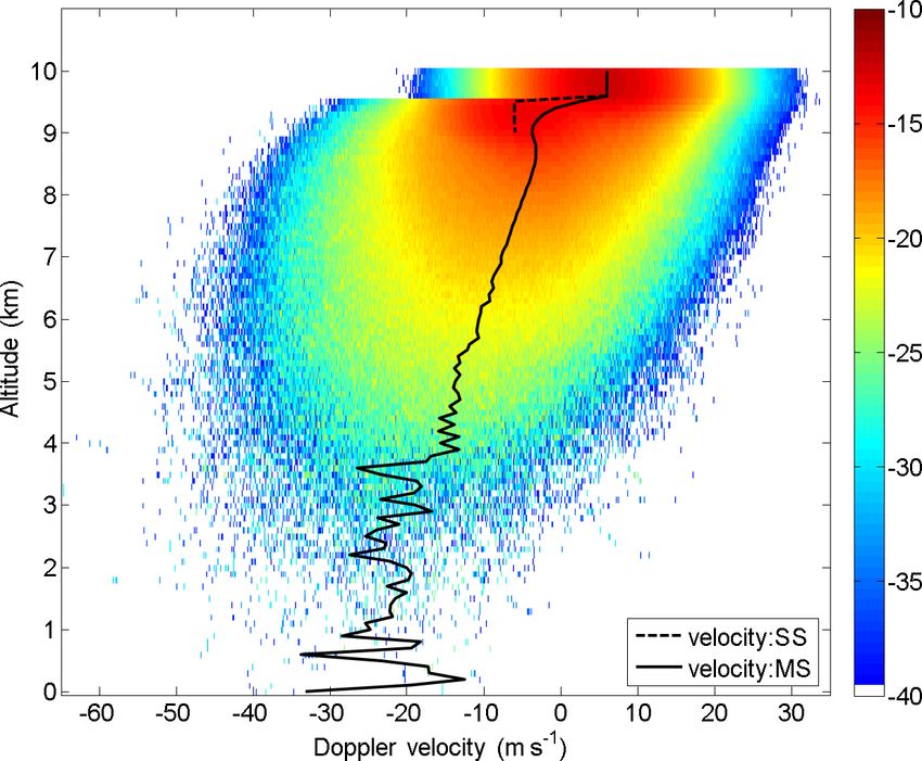
202                                                F. Szczap et al.: McRALI: a Monte Carlo high-spectral-resolution simulator

Figure 1. Schematic presentation of the McRALI-FR simulator. Once the simulation conditions are defined (step 1), McRALI calculates the
idealized backscatter spectrum (step 2). In the last step (step 3), using dedicated software, the desired quantity profiles are calculated. Note
that cloud extinction between 9 and 10 km of altitude is set to 3 km−1 for both the lidar and radar simulation.

Eq. (4) takes the form                                                    where k i is the unit director vector defined between the scat-
                                                                        terer i and i + 1.
               1
fr = fs 1 − (v r − v s ) · k̂ s,r ,                              (5)         Figure 2 shows a schematic diagram of the frequency
               c                                                          shift consideration at each interaction by using the local esti-
where the terms of the second order or higher than 1/c are                mate method. A photon path of two scattering events within
neglected.                                                                the lidar–radar FOV is represented in red. The velocity of
   In multiple-scattering conditions, Eq. (5) can be rewritten            the first and the second scatterer is v 1 and v 2 , respectively.
for the scattering order i as follows:                                    At the first and second scattering, the frequency shift is
                                                                        1f1 = fc0 v 1 · (k 0 − k 1 ) and 1f2 = fc0 v 2 (k 1 − k 2 ), respec-
                 1                                                        tively. At each scattering event, McRALI-FR uses the local
fi+1 = fi 1 − (v i+1 − v i ) · k̂ i,i+1 , i = 0, 1, . . ., n, (6)
                 c                                                        estimate method to compute the contribution to the detec-
where n is the total number of scattering orders. The fre-                tor. For example, at the second scattering event, the total fre-
quency f0 of an emitted photon and the vector v 0 = v n+1 =               quency shift is computed as 1f2;total = 1f1 +1f 0 2 +1f 0 sat ,
                                                                          where 1f 0 2 = fc0 v2 k 1 − k 0 2 , with k 0 2 being the direction

v sat of the satellite velocity belong to the set of input param-
eters for McRALI-FR.                                                      from the second scattering event to the detector (dotted blue
    In general, if a photon was scattered by particles n times,           line), which works with the local       estimate method, and where
                                                                          1f 0 sat = − fc0 v sat k 0 − k 0 2 , with v sat being the satellite ve-

its frequency at the lidar–radar receiver is expressed as fol-
lows:                                                                     locity. The frequency shift due to satellite motion is deliber-
           "
                     n
                                                 #                        ately ignored to simplify the scheme, but it is present in the
                 1X                                                       codes. Computation of the McRALI-FR power spectrum can
fn = f0 1 −             (v i+1 − v i ) · k̂ i,i+1 .            (7)
                 c i=0                                                    also be performed following the convention of the “Gaussian
                                                                          approach” proposed by Battaglia and Tanelli (2011).
All terms of the second order or higher than 1/c are neglected               Note that in the current version of McRALI-FR codes, the
as above. The unit vector k̂0,1 is directed from the satellite to         wind velocity can be set by the user or provided by large eddy
the first scatterer; k̂n,n+1 is directed from the last scatterer to       simulation models at their grid scale. Sub-grid turbulence
the satellite. It should be noted that Eq. (7) is in agreement            wind velocity is assumed to be homogeneous and isotropic;
with Eq. (5) of the work by Battaglia and Tanelli (2011),                 the turbulence velocity vector v turb is distributed according to
wherein, at the scattering order i, the frequency shift 1fi               a Gaussian probability density function (PDF) (see Wilczek
can also be given by                                                      et al., 2011, and references therein). The single-point veloc-
        f0                       f0                                      ity PDF has zero mean and the standard deviation σturb for
1fi =      v i k i−1,i − k i,i+1 = v i (k i−1 − k i ) ,          (8)
        c                         c

Atmos. Meas. Tech., 14, 199–221, 2021                                                          https://doi.org/10.5194/amt-14-199-2021
F. Szczap et al.: McRALI: a Monte Carlo high-spectral-resolution simulator                                                         203

                                                                      the transmitter, calculated in the same way as Battaglia et
                                                                      al. (2006), are given by

                                                                      u0 = a1 cos 20 cos φ0 − a2 sin φ0 + a3 sin 20 cos φ0 ,     (12.1)
                                                                      v0 = a1 cos 20 sin φ0 + a2 cos φ0 + a3 sin 20 sin φ0 ,     (12.2)
                                                                      w0 = −a1 sin 20 + a3 cos 20 ,                              (12.3)
                                                                                                   1/2                           1/2
                                                                      where a1 = x1 1 + x12 + x22       , a2 = x2 / 1 + x12 + x22      ,
                                                                                        2     2
                                                                                                1/2
                                                                      and a3 = 1/ 1 + x1 + x2        with x1 = tan η and x2 = tan ξ .
                                                                      To reproduce the Gaussian pattern of Eqs. (9) and (11), η and
                                                                      ξ are Gaussian-distributed random numbers
                                                                                                              √      with zero√mean
                                                                      and standard deviation equal to θlaser / 2 and θFOV / 2ln2,
                                                                      respectively. The multivariate normal distribution is gener-
Figure 2. Schematic diagram of the frequency shift consideration
                                                                      ated using the Box–Muller method (see, e.g., Tong, 1990).
along the propagation of photons in scattering medium in the frame-
work of the locate estimate method.                                   2.4   Modeling of a Lambertian surface

                                                                      The current version of the McRALI-FR code uses the Lam-
all three coordinates of v turb . The multivariate normal distri-     bertian surface model. The probability that a photon is scat-
bution is generated using the Box–Muller method (see, e.g.,           tered by the surface is defined by the albedo 3. When 3 = 0,
Tong, 1990).                                                          i.e., the black surface model, it is assumed that all photons are
                                                                      absorbed by the surface. Otherwise, i.e., 0 < 3 ≤ 1, the pho-
2.3   Modeling of transmitter and receiver pattern                    ton weight is multiplied by 3. All photons scattered by the
                                                                      Lambertian surface are depolarized, i.e., have Stokes param-
The current version of the McRALI-FR codes only allows                eters of the form S = [I, 0, 0, 0]. The interaction of a photon
the monostatic configuration of transmitters and receivers of         with the surface is treated in the same way as scattering by
lidar or radar systems. Lidar–radar systems can be positioned         a cloud or aerosol particle or the Rayleigh scattering (Cornet
at any altitude, allowing for ground-based, spaceborne, and           et al., 2010).
airborne configurations with any viewing direction. The li-              First, the new direction of a photon scattered by the surface
dar transmitter is assumed to be a Gaussian laser beam with           is random and it is simulated according to the well-known
1/e angular half-width θlaser . For instance, a Gaussian laser        algorithm (see, e.g., Mayer, 2009). The azimuth angle ϕ is
beam pattern with 1/e angular half-width θlaser is described          chosen randomly between 0 and 2π .
by (Hogan, 2008)
              "            !#                                         ϕ = 2π q1                                                    (13)
                     θ2
g1 (θ) = exp − 2              .                            (9)        As for the zenith angle θ , its cosine µ = cos(θ ) is randomly
                    θlaser
                                                                      drawn using the expression
   The lidar receiver is assumed to be a top-hat telescope with            √
a half-angle field of view θFOV , and its pattern can be de-          µ = − q2 ,                                                   (14)
scribed by (Hogan and Battaglia, 2008)
                                                                      where q1 and q2 are uniform random numbers between 0
                                                                      and 1.

             1 ; θ ≤ θFOV
g2 (θ) =                                                   (10)          Secondly, the local estimate technique (Marchuk et al.,
            0 ; θ > θFOV .
                                                                      1980) is implemented to calculate at each scattering point
Radar transmitters and receivers are assumed to be Gaussian           the contribution of the photon in the direction of the sensor.
antennas with a 3 dB half-width θFOV . For instance, a Gaus-             Figure 3 shows as an example of the two lidar signals as a
sian antenna pattern with 3 dB half-width θFOV is described           function of the distance from the lidar position for two view-
by (Battaglia et al., 2010)                                           ing directions (nadir and inclined at 24.7◦ , chosen so that
             "               !#                                       the distance to the ground is 11 km). The lidar altitude is
                         θ2                                           10 km, the laser divergence is 0.0007, and the field of view
g3 (θ) = exp −ln2 2             .                       (11)
                        θFOV                                          of the receiver is 0.005 rad. An aerosol layer between alti-
                                                                      tudes of 2 and 3 km has an optical thickness of 0.15. The
   The lidar and radar transmitter and receiver pointing di-          single-scattering albedo of 0.91888 and the phase function
rection is defined by the zenith 20 and azimuthal φ0 angles.          were computed with the refractive index and microphysical
Direction cosines (u0 , v0 , w0 ) of the initial photon leaving       parameters of the coarse mode of desert dust, assuming that

https://doi.org/10.5194/amt-14-199-2021                                                    Atmos. Meas. Tech., 14, 199–221, 2021
204                                                 F. Szczap et al.: McRALI: a Monte Carlo high-spectral-resolution simulator

                                                                         with inclined sighting by taking into account the properties
                                                                         of the Lambertian surface, but also the mirror images (as it
                                                                         is seen in certain radar observations). It should be noted that
                                                                         to make the mirror image appear in this simulation, we have
                                                                         imposed a maximum surface albedo equal to 1.

                                                                         2.5     Doppler radar CPR/EarthCARE configuration

                                                                         2.5.1    Modeling gas absorption

                                                                         At 94 GHz (3.2 mm, W band), the attenuation by atmospheric
                                                                         gas is mainly due to absorption of water vapor and oxygen
                                                                         (Liebe, 1985; Lenoble, 1993; Liou, 2002). The attenuation A
                                                                         (in dB km−1 ) by water vapor and oxygen in McRALI codes
                                                                         is computed from Liebe (1985) tabulations. Absorption coef-
                                                                         ficient σabs (in km−1 ) is given by σabs = 0.2303 A. Absorp-
                                                                         tion and scattering are treated separately in McRALI codes,
Figure 3. Profiles of the attenuated backscatter (ATB) coefficient       as is done in 3DMCPOL (Fauchez et al., 2014), whereby ab-
(black – nadir-looking, red – inclined at 24.7◦ ) as a function of the   sorption is considered by a photon weight wabs according
distance from the lidar position. The lidar altitude is 10 km.           to the Lambert–Beer law (Partain et al., 2000; Emde et al.,
                                                                         2011):
                                                                                     Rs
                                                                         wabs = e−     0 σabs   (s 0 )ds 0 ,                           (15)
particles are spheroids with a distribution of the aspect ratio
(Dubovik et al., 2006). The albedo of the Lambertian surface             where ds 0 is a path element of the photon path.
is set to 1.
   For the nadir direction example, the layer at distances be-           2.5.2    Doppler spectrum and its relation to reflectivity,
tween 7 and 8 km that exhibits large values of the backscat-                      Doppler velocity, and spectral width
ter coefficient corresponds to the aerosol layer between 2 and
3 km in altitude. At a distance of 10 km, the very large value           The Doppler radar community uses the Doppler spectrum
of the backscatter coefficient corresponds to the echo from              S(r, v), a power-weighted distribution of the radial velocities
the surface. Then, for distances larger than 10 km, the lidar            v in the velocity range dv of the scatterers (Doviak and Zrnić,
signal drastically decreases. But for the distances from 12              1984). McRALI-FR codes dedicated to Doppler radar simu-
to 13 km, another layer can be observed. That layer corre-               lations compute S(r, v) by using the first Stokes parameter
sponds to a third and higher order of scattering. In this partic-        I (r, f ) and the Doppler formula v = cf/2f0 . We follow the
ular case, the triple scattering is of the type “surface–aerosol         convention that the Doppler velocity is positive for motion
layer–surface”. It is also called the mirror image and refers            away from the radar. The backscattering coefficient profile
to reflectivities measured by airborne or spaceborne radars at           β (r) is then given by
ranges beyond the range of the surface reflection (see, e.g.,                      Z+∞
Battaglia et al., 2010). It should be underscored that the mir-          β(r) =       I (r, v) dv.                                     (16)
ror image disappears when, during a simulation, one photon
                                                                                  −∞
can undergo no more than two scatterings. The same behav-
ior is observed for the case of the inclined viewing direc-                 The reflectivity Z (r) profile is computed using Eq. (3) and
tion. The position of the aerosol layer, the surface echo, and           β (r). The Doppler velocity profile VDop (r) is defined as
the mirror image shifts in agreement with corresponding dis-                         R +∞
tances from the lidar.                                                                     vI (r, v) dv
   The signal-to-noise ratio (SNR) of lidars is generally much           VDop (r) = R−∞ +∞              ,                           (17)
lower than the SNR of radars. Thus, in practice it is im-                              −∞ I (r, v) dv

possible to observe a mirror image with a spaceborne lidar,              and the Doppler velocity spectral width profile σDop (r) is
contrary to a spaceborne radar. Results presented in Fig. 3              obtained from
should be considered a numerical and theoretical exercise                           R +∞             2
that demonstrates the McRALI capacities. The simulations                  2          −∞ v − VDop (r) I (r, v) dv
                                                                         σDop (r) =        R +∞                  .              (18)
were performed with a very high number of photon trajec-
                                                                                            −∞ I (r, v) dv
tories so that the numerical noise of the McRALI simulator
is very low. Under these idealized simulation conditions, we               Figure 4 shows, as an example, a simulation of the
show that McRALI is able to simulate lidar–radar systems                 Doppler power spectrum, the Doppler velocity, the Doppler

Atmos. Meas. Tech., 14, 199–221, 2021                                                               https://doi.org/10.5194/amt-14-199-2021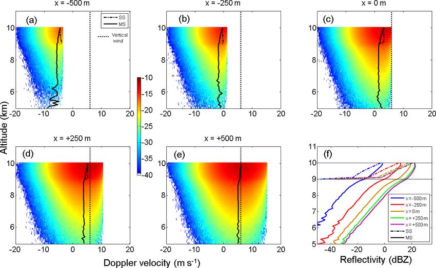
F. Szczap et al.: McRALI: a Monte Carlo high-spectral-resolution simulator                                                            205

velocity spectral width, and the reflectivity profiles for a
CPR/EarthCARE-like radar for a homogenous iced cloud
layer with fixed 6 m s−1 downdraft at all altitudes (see de-
tails of the conditions of the simulation in Table 1) with
(σturb = 0.5 ms−1 ) and without (σturb = 0 ms−1 ) sub-grid tur-
bulent wind. In a first step, McRALI-FR codes dedicated
to Doppler radar simulations compute the idealized Doppler
power spectrum density S(rv). The first Stokes parameter
I (r, v) of the Doppler spectrums (with and without sub-grid
turbulent wind) are shown in Fig. 4a and b, respectively.
Then, in a second step, software computes the reflectivity,
the Doppler velocity, and the Doppler velocity spectral width
profiles with Eqs. (16), (17), and (18), respectively. Multiple-
scattering (MS) and single-scattering (SS) Doppler velocity
profiles are superimposed on the MS Doppler spectrum. MS
and SS Doppler velocity values are constant within the cloud
layer (between 9 and 10 km of altitude) and are equal to the
“true” 6 ms−1 vertical velocity, whatever the wind turbulence       Figure 4. Estimated Doppler spectrum moments for a Doppler
value is. Due to multiple-scattering processes, the apparent        CPR/EarthCARE-like radar. (a) Doppler spectrum without wind
Doppler velocity of 6 ms−1 can be observed between the              turbulence. Doppler velocity profiles are superimposed (MS: dot-
cloud-base altitude and the ground, contrary to the SS appar-       ted line, SS: cross). (b) Same as (a), but with wind turbulence.
ent Doppler velocity, which appears only in the cloud layer.        (c) Vertical profiles of MS (full lines) and SS (crosses) Doppler
                                                                    spectrum width with wind turbulence (red) and without wind turbu-
   In Fig. 4c the MS and SS Doppler velocity spectral width
                                                                    lence (blue). (d) Vertical profiles of MS (full lines) and SS (crosses)
profiles are drawn. Under the SS approximation, the Doppler         reflectivity with wind turbulence (red) and without wind turbulence
velocity spectral width σDop is given by (Kobayashi et al.,         (blue). The altitude of the base of the iced homogeneous cloud layer
                                 2 = σ2
2003; Battaglia et al., 2013) σDop                2         2
                                         hydro + σshear + σturb +   (optical depth of 3) is 9 km. Its geometrical thickness is 1 km.
  2
σmotion , where σhydro is due to the spread of the terminal
fall velocities of hydrometeors of different size, σshear is the
broadening due to the vertical shear of vertical wind, σturb is     2.6     High-spectral-resolution (HSR) lidar
the broadening of the vertical wind due to turbulent motions                ATLID/EarthCARE configuration
in the atmosphere, and σmotion is the spread caused by the
coupling between the platform motion and the vertical wind          2.6.1     Modeling of the emitted laser energy spectrum
shears of the horizontal winds. For a Gaussian circular an-
tenna pattern, assuming zero fall velocities of hydrometeors        The laser transmitter of the ATLID instrument has spec-
and no wind shear, σDop is given by (Tanelli et al., 2002)          tral requirements with a spectral line width below 50 MHz
                                                                    (Hélière et al., 2017). In McRALI-FR codes, the frequency of
                                   2
                                                                    the emitted radiation is drawn randomly according to a Gaus-

 2         2           θFOV vsat
σDop   = σturb +        √               ,                   (19)    sian law of average f0 with a 1/e half-width σf0 = 50 MHz.
                       2 ln (2)
where vsat is the satellite velocity relative to the ground and     2.6.2     Modeling of thermal molecular velocity
θFOV is the Gaussian (3 dB) FOV half-angle.                                   distribution
   Simulated SS Doppler velocity spectral widths with-
out turbulence and with turbulence are close to 3.58 and            The current version of McRALI-FR codes assumes that each
3.62 m s−1 , respectively. Both computed values are very            component of molecular velocity is distributed according to
close to theory-predicted values. On the other hand, MS pro-        the Maxwell–Boltzmann density function with null mean and
cesses together with sub-grid turbulent wind are a source           standard deviation a given by
of broadening. For example, at 2 km under the cloud base,                 r
σDop = 3.75 m s−1 , which is larger than the SS value.                        kT
   Vertical profiles of MS and SS reflectivity are shown in         a=           ,                                                    (20)
                                                                              m
Fig. 4d. These profiles are not sensitive to the wind turbu-
lence. MS processes are a source of enhancement of the re-          where k is the Boltzmann’s constant, T is the temperature,
flectivity compared to the SS reflectivity and the apparent         and m is the molecular mass of gas. The multivariate nor-
reflectivity that can be observed under the cloud layer.            mal distribution is generated using the Box–Muller method.
                                                                    As a next step, we plan to take into account spontaneous
                                                                    Rayleigh–Brillouin scattering.

https://doi.org/10.5194/amt-14-199-2021                                                    Atmos. Meas. Tech., 14, 199–221, 2021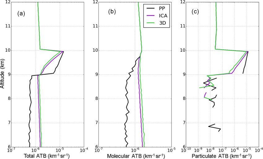
206                                            F. Szczap et al.: McRALI: a Monte Carlo high-spectral-resolution simulator

2.6.3   Relation of the HSR spectrum to molecular and              and Cma , respectively). The calculation method of these co-
        particulate backscattering coefficient: modeling           efficients is described in detail in Shipley et al. (1983). As an
        of a Fabry–Pérot interferometer                            indication, for the present study in the ATLID/EarthCARE
                                                                   lidar configuration, these coefficients have the following val-
One of the important features of HSR lidars is the possibility     ues: Cmm = 0.543, Cma = 0.457, Caa = 0.998, and Cam =
to retrieve profiles of particle extinction and the backscatter-   0.002. Note that the cross-talk coefficients used in this pa-
ing coefficient without the need for additional information on     per assume ideal behavior of the ATLID FP interferometer.
the lidar ratio (Shipley et al., 1983; Ansmann et al., 2007, and   In practice, the Airy function will be “blurred” due to the
references therein). HSR technology relies on the principle        effects of nonideal collimation of the beam, frequency jit-
of measuring the Doppler frequency shift resulting from the        ter, surface roughness, and so on. All these factors combine
scattering of photons by molecules (referred to as molecular       to decrease the peak transmission and lower the full-width
scattering or Rayleigh scattering) and by particles (referred      at half-maximum (see the Fig. 9 in Pereira do Carmo et al.,
to as particulate scattering or Mie scattering). The character-    2019). It is important to keep in mind that all the calculations
istic shape of the HSR spectrum depends on both these two          shown in this paper are merely “EarthCARE-like” but with
scattering processes: a broad spectrum of low intensity for        an idealized modeled FP interferometer.
molecule scattering and a narrow peak of large intensity for          Figure 5 shows particulate and molecular ATB profiles for
particle scattering.                                               an ATLID/EarthCARE-like lidar. We consider in this exam-
   The spectral width of the particle peak will be determined      ple an ice cloud corresponding to a homogenous layer with
by the spectral width of the laser pulse itself along with         an optical depth 3 between 9 and 10 km in altitude (see de-
any turbulence present in the sampling volume. The spec-           tails of the simulation conditions in Sect. 3.1). In the first
tral width of the ATLID laser will be on the order of 50           step, McRALI-FR codes, dedicated to HSR lidar simula-
MHz so that the laser line width will be the dominant factor.      tions, compute the HSR spectrum S(rf ). The first Stokes pa-
Thus, the molecular backscatter will be much broader than          rameter I (r, f ) of the MS HSR spectrum is shown in Fig. 5a.
the particulate-scattering return. This is due to the fact that    The peak of intensity (in red) centered at 0 GHz between
atmospheric molecules have a large thermal velocity. Assum-        9 and 10 km of altitude corresponds to the position of the
ing a Gaussian molecular thermal velocity distribution with        cloud. It is the contribution of the cloud particles (the so-
a half-width at 1/e of the maximum, molecular broadening           called “Mie contribution”). This spectrum is also character-
γm can be written (Bruneau and Pelon, 2003) as                     ized by the molecular contribution (Rayleigh contribution).
          r                                                        The intensity of the spectrum below the cloud is lower than
        2 2kT
γm =              .                                         (21)   the intensity of the spectrum above the cloud due to particu-
       λ0     m                                                    late extinction. In Fig. 5b, the MS (computed with McRALI-
   If T = 230 K, then γm is of the order of 2 GHz, which is        FR) and SS (computed from SS theory) vertical profiles of
about 40 times larger than the laser line width. Thus, using       spectral width are represented. We note very good agreement
interferometers (such as the Fabry–Pérot (FP) interferometer       between the SS theoretical and MS simulated values at both
equipping the ATLID/EarthCARE lidar) and appropriate sig-          the cloudy and molecular levels. This suggests that MS ef-
nal processing (Hélière et al., 2017), the molecular and par-      fects have very little impact on spectral width. Then, in a sec-
ticulate contributions of the lidar backscattered signal can be    ond step, a simulated FP interferometer separates the partic-
separated. Then particulate and molecular backscattering co-       ulate contribution from the molecular contribution and pro-
efficient profiles (attenuated or apparent attenuated backscat-    vides the vertical profiles of particulate and molecular ATB
tering coefficient or simply attenuated backscatter, also de-      as shown in Fig. 5c. The total ATB calculated directly from
noted as ATB) can be separately determined. In this study,         the spectrum, SS molecular, and SS particulate backscatter
we suppose that the FP interferometer has the following pa-        profiles is also represented. Above the cloud, particulate ATB
rameters. The free spectral range is 7.5 GHz, the finesse is       is not strictly zero and molecular ATB is not strictly equal to
10, and the FP is centered at the wavelength 355 nm. The           total ATB because of the FP remaining cross-talk effects (see
cross-talk effects were taken into account according to the        above). In the cloudy part between 9 and 10 km of altitude,
work by Shipley et al. (1983). The coefficients of the cross-      the molecular and particulate ATB logically decrease expo-
talk correction were computed using an Airy function (see,         nentially with depth. The SS backscatter profiles decrease
e.g., Vallée and Soares, 2004), which describes the FP trans-      faster with depth than the MS backscatter profiles, revealing
mission spectrum, assuming a Gaussian molecular thermal            that MS effects on ATB are not negligible. Under the cloud,
velocity distribution with a half-width at 1/e of the maxi-        molecular ATB is almost equal to total ATB. It is likely worth
mum γm (Eq. 21). This method determines four calibration           pointing out the quasi-exponential decay of the below-cloud
coefficients corresponding to the fraction of cloud–aerosol        molecular return towards single-scattering levels. This result
backscatter in the molecular and particulate channels (Cam         is consistent with the cases shown by Donovan (2016). Par-
and Caa , respectively), as well as the fraction of molecular      ticulate ATB is almost zero. Some nonzero values exist due
backscatter in the molecular and particulate channels (Cmm

Atmos. Meas. Tech., 14, 199–221, 2021                                                 https://doi.org/10.5194/amt-14-199-2021
F. Szczap et al.: McRALI: a Monte Carlo high-spectral-resolution simulator 207
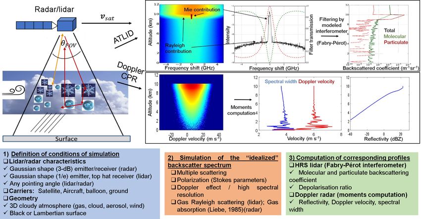
Figure 5. (a) Vertical profile of MS HSR spectrum for an ATLID-
like lidar. (b) Spectral width profiles. SS and MS spectral width
profiles computed by McRALI (circle) are in green and red, respec-
tively. Theoretical SS molecular and SS particulate width profiles Figure 6. Schematic representation of two specific positions of a
(full line) are in black and blue, respectively. (c) Vertical profiles of spaceborne lidar–radar system relative to the idealized box cloud.
the MS (line) and SS (circle) backscattered coefficient (ATB). To- The box-cloud base altitude is 9 km, its geometrical thickness is
tal, molecular, and particulate signals are in black, green, and red, 1 km, and its x-horizontal and y-horizontal extension is 2 km and in-
respectively. The altitude of the base of the iced homogeneous cloud finite, respectively. The cloud vertical extinction profile is constant.
layer (optical depth of 3) is 9 km. Its geometrical depth is 1 km. In the two positions, single- and multiple-scattering photon path ex-
amples are represented by green and red arrows, respectively.
to FP cross-talk effects but also due to Monte Carlo noise and
MS processes.
neous within the box cloud. When the lidar–radar system is
3 Assessment of errors induced by NUBF on lidar and just above the cloud edge, the NUBF effect can be signifi-
radar data cant, whereas it is null when the system is completely over
the cloud. Table 1 summarizes the conditions of McRALI-FR
The objectives of this section are to investigate the effects of simulations for data from the HSR ATLID lidar and Doppler
a cloudy atmosphere having 3D spatial heterogeneities un- CPR radar of the EarthCARE mission when the heteroge-
der a multiple-scattering regime on HSR lidar and Doppler neous box cloud is considered.
data by using McRALI-FR simulators. One of the simplest At a wavelength of 355 nm (lidar configuration), gas scat-
shapes of heterogeneous cloud to study this kind of effects is tering properties are based on Hansen and Travis (1974).
the idealized “step” cloud defined in the international Inter- Gas Doppler broadening is computed assuming a Maxwell–
comparison of 3D Radiation Codes (I3RC) phase 1 (Cahalan Boltzmann distribution as presented in Sect. 2.4.1. The scat-
et al., 2005). The main interest is to model behavior in the tering matrix was computed for a gamma size distribu-
vicinity of the single isolated jump in optical depth. With tion of ice crystals having an effective diameter of 50 µm
this in mind, we prefer to use an even more simplistic cloud and the aspect ratio of 0.2. The refractive index value was
model, the box cloud, described in the following paragraph. 1.3243 + i × 3.6595 × 10⁻⁹ ; the surface of particles was as-
A detailed statistical analysis at different averaging scales of sumed to be rough (Yang and Liou, 1996). Optical charac-
representative fine-structure 3D cloud field effects on lidar teristics were computed using the improved geometric optics
and radar observables is beyond the scope of this paper and method (IGOM) (Yang and Liou, 1996). The asymmetry pa-
will be investigated in a future work. rameter is g = 0.73, which is in agreement with experimen-
tal data for cirrus clouds (Gayet, 2004; Shcherbakov et al.,
3.1 Conditions of simulation and definition of the box 2006). Single-scattering albedo is set to 1.0.
cloud At 94 Ghz (radar configuration), we assumed a Henyey–
Greenstein phase function with an asymmetry parameter g =
The box-cloud base altitude is 9 km, its geometrical thick- 0.6. Single-scattering albedo is set to 0.98. These last two
ness is 1 km, and its x-horizontal and y-horizontal extension values are taken from Battaglia and Tanelli (2011) for a sce-
is 2 km and infinite, respectively. Temperature and pressure nario involving a deep convective core with graupel. Wind
vertical profiles assume 1976 US standard atmosphere mod- vertical velocity (downdraft) is set to 6 ms−1 . We assume
els. Optical cloud properties are characterized by the extinc- no wind turbulence nor particle sedimentation velocity. For
tion coefficient set to 0.1, 1.0, and 3 km−1 . a cloud layer at an altitude of around 9 km, the pressure,
Figure 6 shows a representation of two specific positions temperature, and relative humidity can be set to 308 hPa,
of a spaceborne lidar–radar system relative to the idealized 229.7 K, and 100 %, respectively (1976 US standard atmo-
box cloud. Cloud optical properties are spatially homoge- sphere); then gas absorption σabs ≈ 2 × 10⁻⁵ km−1 . We as-
https://doi.org/10.5194/amt-14-199-2021 Atmos. Meas. Tech., 14, 199–221, 2021
208                                             F. Szczap et al.: McRALI: a Monte Carlo high-spectral-resolution simulator

sumed that this value is small enough to neglect the gas ab-        x-horizontal component, then 1v = −vsat kx . Assuming that
sorption for the simulations carried out in this work.              satellite is at the x-horizontal d distance to the box-cloud
   Spacecraft velocity and altitude are set to vsat =               edge and at the z-vertical D distance above the cloud, with
7.2 km s−1 and 393 km, respectively. The lidar–radar system         a vertical (downdraft) wind velocity vwind fixed at 6 ms−1 ,
                                                                                                    1/2
pointing angle is set to 0◦ . The lidar transmitter is assumed      then vcrit = −vsat d/ d 2 + D 2      +vwind . For x = −500, x =
to be a Gaussian laser beam with 1/e angular half-width             −250, x = 0, x = 250, and x = 500 m, vcrit = −3.4, vcrit =
θ = 22.5 µrad. The lidar receiver is assumed to be a top-hat        −1.3, vcrit = 6, vcrit = 10.7, and vcrit = 15.4 m s−1 , respec-
telescope with a half-angle field of view θFOV = 32.5 µrad,         tively. These values are very close to those estimated from
which represents a ground beam footprint of around 30 m.            the five respective power spectra in Fig. 7.
Radar transmitters and receivers are assumed to be Gaussian            Figure 7f also shows the five reflectivity profiles corre-
antennas with a 3 dB half-width θ = θFOV = 0.0475◦ , which          sponding to the five positions of the satellite relative to the
represents a ground beam footprint of around 660 m.                 edge of the box cloud. MS reflectivity profiles are larger than
   McRALI-FR code simulates the multiple-scattering and             SS reflectivity profiles because MS processes logically in-
single-scattering idealized HSR and Doppler spectrum for li-        crease the reflectivity value. We can also see MS effects on
dar and radar configurations, respectively. Lidar spectra are       the apparent reflectivity that is non-null under the cloud layer,
computed for five positions (x-horizontal ground-projected          contrary to the SS apparent reflectivity. At the same time,
distance) relative to the box-cloud edge. Lidar position val-       as the satellite approaches the edge of the cloud and keeps
ues are x = −8.6, −4.0, 0, 4.0, and 8.6 m. Indeed, the ratio        moving forward, SS and MS apparent reflectivity profile val-
(we also talk about cloud coverage) of the cloudy part in-          ues increase due to the fact that the NUBF effect decreases.
side the ATLID lidar FOV divided by the full lidar footprint        Many studies have focused on the NUBF effect on rain fields
area at the altitude of 10 km is 10 %, 30 %, 50 %, 70 %, and        retrieved by radar from space (Amayenc et al., 1993; Testud
90 %, respectively. Then, software computes apparent molec-         et al., 1996; Durden et al., 1998; Iguchi et al., 2009). Iguchi et
ular and particulate backscattering coefficient profiles, as-       al. (2000) showed that the NUBF effect could be accounted
suming that the ATLID/EarthCARE lidar is equipped with              for by a factor determined from horizontal variation of the at-
FP interferometers (see Sect. 2.5.3). For the radar config-         tenuation coefficient. Our simulations are coherent with the
uration, simulations are carried out every 100 m; Doppler           literature. A detailed investigation of the NUBF effect on re-
spectra are computed for position values fixed at x = −500,         flectivity profiles for spaceborne cloud radar will be carried
−250, 0, 250, and 500 m. Then, software computes reflectiv-         out in a later work.
ity, Doppler velocity, and Doppler velocity spectrum width
profiles with the help of Eqs. (16), (17), and (18).                3.2.2   NUBF effects on Doppler velocity and Doppler
                                                                            spectrum width
3.2     CPR/EarthCARE configuration
                                                                    Figure 7 shows the SS and MS vertical profiles of Doppler
3.2.1    NUBF effects on Doppler radar data: Doppler                velocity superimposed on the five power spectra for the five
         spectrum and reflectivities                                positions of the satellite relative to the box-cloud edge: x =
                                                                    −500, −250, 0, 250, and 500 m. Since each power spectrum
Figure 7a–e show vertical profiles of MS radar Doppler              has no value beyond the vcrit velocity, which is due to the
spectra density in the CPR/EarthCARE configuration corre-           NUBF effect, it is obvious that the profile of the apparent
sponding to the five positions of the satellite relative to the     Doppler velocity is different from the profile of the vertical
edge of the box cloud with optical depth set to 3. Regard-          wind velocity fixed at 6 ms−1 . Figure 8 shows the MS and
less of the satellite position, Doppler spectra correspond to       SS apparent Doppler velocity and Doppler spectrum width
negative Doppler velocity values. This is consistent with the       computed every 100 m along the horizontal axis. These quan-
convention that the Doppler velocity is positive for motion         tities are estimated at different altitudes (cloud top, middle,
away from the radar. As the satellite approaches the edge           and base) and are plotted as a function of the satellite dis-
of the cloud and carries on, the NUBF effect decreases. In-         tance to the box-cloud left edge. Differences between appar-
deed, the Doppler spectrum becomes more and more sym-               ent Doppler velocities are in general small (around 1 m s−1 )
metrical. The asymmetric shape of the Doppler spectrum is           whatever the altitude is, and differences between MS and SS
due to zero values beyond a critical value of Doppler veloc-        Doppler velocities are also small, no larger than 1 m s−1 at
ity vcrit . As an example, vcrit ≈ −3.4 ms−1 in Fig. 7a. The        the bottom of the cloud. The same conclusions can be drawn
explanation of the vcrit value is purely geometric. Doppler         for the Doppler spectrum width at which differences are no
broadening is dominated by Doppler fading due to satellite          larger than 0.3 m s−1 . This implies that MS processes do
motion. Under the SS approximation, neglecting wind ve-             not play an important role in the estimation of the apparent
locity, the Doppler shift is given by 1v = 1/2v sat k 0 − k 0 1 ,

                                                                    Doppler velocity or in the estimation of apparent spectrum
with k 0 = −k 01 . Assuming v sat with an x-horizontal positive     width (for the specific conditions of simulation with the box
component, k 0 , in the (z–x) vertical plan and with kx as the      cloud) compared to the NUBF effect. The NUBF Doppler

Atmos. Meas. Tech., 14, 199–221, 2021                                                  https://doi.org/10.5194/amt-14-199-2021
F. Szczap et al.: McRALI: a Monte Carlo high-spectral-resolution simulator 209
Table 1. Description of the simulation conditions presented in this work. This table summarizes the characteristics of the ATLID/EarthCARE-
type lidar and the CPR/EarthCARE-type radar as well as properties of a cloudy atmosphere and quantities computed by McRALI-FR codes.
ATLID/EarthCARE-type lidar CPR/EarthCARE-type radar
Characteristics of lidar and radar systems
Spacecraft altitude 393 km 393 km
Projected spacecraft velocity 7.2 kms−1 7.2 kms−1
Wavelength or frequency 355 nm 94 GHz
Pointing angle 0◦ 0◦
Emitter model and beam half-width Gaussian (1/e), 22.5 µrad Gaussian (3 dB), 0.0475◦
Receiver model and FOV half-angle Top hat, 32.5 µrada Gaussian (3 dB), 0.0475◦
Beam footprint ∼ 26 m ∼ 650 m
Characteristics of a cloudy atmosphere
Temperature and pressure vertical profiles US standard atmosphere model (1976) No gasd
Gas optical properties vertical profile Hansen and Travis (1974) No gasd
Gas Doppler broadening Maxwell–Boltzmann distribution –
Geometry of box-cloud model x wide = 2 km, y depth = 100 km, z thickness = 1 km
Cloud-top and cloud-base altitude 9–10 km
Cloud geometrical depth 1 km
Cloud extinction 0.1, 1.0, 3 km−1
Single-scattering albedo 1.0 0.98
Cloud phase function Reff = 25 µm (Yang and Liou, 1996) Henyey–Greenstein
Rough ice crystals
Asymmetry parameter 0.73 0.6
Interferometer Fabry–Pérot –
Vertical wind velocity 0 ms−1 6 ms−1 (downdraft)e
Wind turbulence (standard deviation σturb 0 ms−1 0 ms−1
of Gaussian isotropic model)
Particle sedimentation velocity 0 ms−1 0 ms−1
Simulated quantities from idealized range- and frequency-resolved Stokes parametersb
Relative horizontal position of the lidar– x = −8.6, −4.0, 0, 4.6 and 8.6 m x = −500, −250, 0, 250 and 500 mf
radar system to the cloud edge
Power spectrum profiles High-spectral-resolution spectrum Doppler spectrum
Vertical profiles Backscatter, depolarization ratio Width, reflectivity
Molecular, particle, and total Doppler velocity, Doppler spectral
Vertical resolutionc 100 m 100 m
Power spectrum interval resolution 0.01 Hz 1 ms−1
a Other simulations are performed with an FOV half-angle of 325 µrad. b Idealized means that receiver noise, along-track integration, and Nyquist folding are
ignored. c ATLID and CPR vertical resolution is 100 m from −1 to 20 km in height. d Gas absorption (Liebe, 1985) can be taken into account. e A specific case with
a two-layer cloud with 6 and −6 ms−1 vertical wind velocity in the top layer and bottom layer, respectively, is also studied. f For radar configurations, simulations
are also carried out every 100 m according to the horizontal distance.
velocity bias between apparent Doppler velocity and “true” a satellite velocity (i.e., vsat = 7.2 kms−1 ) and the Doppler
vertical wind velocity fixed at 6 m s−1 is around −10, −5, velocity computed with a satellite velocity set to 0 m s−1
−3, −2, and −1 ms−1 at x = −500, −250, 0, 250, 500 m, (Battaglia et al., 2018). Sy et al. (2014) showed that the
respectively. NUBF bias of Doppler velocity is correlated with the hori-
In general the NUBF bias of Doppler velocity can be zontal gradient of reflectivity and demonstrated that the the-
expressed as a function of the distribution of the radar re- oretical proportional coefficient α value is bounded between
flectivity (Tanelli et al., 2002). An estimate of the NUBF 0.165 and 0.219 m s−1 (dBZ km−1 )−1 . Kollias et al. (2014)
bias of Doppler velocity can be obtained by considering estimated this proportional coefficient value close to α =
the difference between the Doppler velocity computed with 0.23 m s−1 (dBZ km−1 )−1 for along-track horizontal integra-
https://doi.org/10.5194/amt-14-199-2021 Atmos. Meas. Tech., 14, 199–221, 2021210 F. Szczap et al.: McRALI: a Monte Carlo high-spectral-resolution simulator
Figure 7. Vertical profiles of MS radar Doppler spectra (logarithm of the spectral density; in m−1 sr−1 (m s−1 )−1 ) in the CPR/EarthCARE
configuration corresponding to the five positions x = −500 m (a), x = −250 m (b), x = 0 m (c), x = +250 m (d), and x = +500 m (e) of the
satellite relative to the edge of the box cloud. SS (black line) and MS (black dotted line) vertical profiles of Doppler velocity are superimposed.
The vertical wind velocity profile (downdraft) fixed at wwind = 6 m s−1 during our simulation is also drawn (black dotted line). (e) The five
reflectivity (in dBZ) profiles (MS: full lines, SS: dotted lines) corresponding to the five positions (x = −500 in blue, x = −250 in red,
x = 0 m in brown, x = 250 m in green, and x = 500 m in magenta) relative to the edge of the box cloud. Cloud optical depth is 3.
depths of the box cloud of 0.1, 1, and 3. We note that the
α value is between 0.14 and 0.16 m s−1 (dBZ km−1 )−1 and
is almost independent of the position of the satellite relative
to the box-cloud edge. If the satellite position is just above
the cloud edge, the proportional coefficient value is close to
0.15 m s−1 (dBZ km−1 )−1 , a value close to that obtained by
Sy et al. (2014).
3.2.3 Effects of vertically heterogeneous wind velocity
on Doppler velocity
A first study of the effects of multiple scattering on the
Doppler velocity vertical profile in the case of vertically het-
Figure 8. MS (full lines) and SS (dotted line) apparent Doppler erogeneous wind velocity is carried out for a very specific
velocity and Doppler spectrum width as a function of the distance of case in the CPR/EarthCARE configuration. Indeed, for a ho-
the satellite relative to the box-cloud left edge. Values are computed mogeneous cloud layer with a base altitude of 9 km and
at cloud top (10 km of altitude, in red), middle (9.5 km of altitude, with a geometrical thickness of 1 km, the vertical velocity
in blue), and base (9 km of altitude, in green). Optical thickness of is set to 6 m s−1 (downdraft) and −6 m s−1 (updraft) in the
the box cloud is 3. Simulations are done every 100 m. upper and lower part of the cloud layer, respectively. Fig-
ure 10 shows vertical profiles of the MS radar Doppler spec-
trum and the MS and SS Doppler velocity profiles computed
tion of 500 m (i.e., Doppler CPR/EarthCARE resolution) and with McRALI-FR. The measured Doppler velocity under the
for all their available simulations performed with a cirrus SS regime (black dotted line in Fig. 10) is equal to 6 m s−1
cloud and a precipitation system. Figure 9 shows the Doppler (−6 m s−1 ) in the upper (lower) part of the cloud, and the
velocity NUBF bias as a function of the horizontal reflec- SS Doppler velocity can be used as the reference of the true
tivity gradient for a horizontal integration of 500 m at four velocity. In the upper part of the cloud, the measured MS
positions relative to the box-cloud edge (−200, 100, 0, and Doppler velocity is 6 m s−1 , which equals the true velocity.
100 m). Computations are carried out for different optical In the lower part of the cloud, the measured MS Doppler ve-
Atmos. Meas. Tech., 14, 199–221, 2021 https://doi.org/10.5194/amt-14-199-2021You can also read