Improved aerosol correction for OMI tropospheric NO2 retrieval over East Asia: constraint from CALIOP aerosol vertical profile - Atmos. Meas. Tech
←
→
Page content transcription
If your browser does not render page correctly, please read the page content below
Atmos. Meas. Tech., 12, 1–21, 2019
https://doi.org/10.5194/amt-12-1-2019
© Author(s) 2019. This work is distributed under
the Creative Commons Attribution 4.0 License.

Improved aerosol correction for OMI tropospheric NO2 retrieval
over East Asia: constraint from CALIOP aerosol vertical profile
Mengyao Liu1,2 , Jintai Lin1 , K. Folkert Boersma2,3 , Gaia Pinardi4 , Yang Wang5 , Julien Chimot6 , Thomas Wagner5 ,
Pinhua Xie7,8,9 , Henk Eskes2 , Michel Van Roozendael4 , François Hendrick4 , Pucai Wang10 , Ting Wang10 ,
Yingying Yan1 , Lulu Chen1 , and Ruijing Ni1
1 Laboratory  for Climate and Ocean-Atmosphere Studies, Department of Atmospheric and Oceanic Sciences,
School of Physics, Peking University, Beijing, China
2 Royal Netherlands Meteorological Institute, De Bilt, the Netherlands
3 Meteorology and Air Quality department, Wageningen University, Wageningen, the Netherlands
4 Royal Belgian Institute for Space Aeronomy (BIRA-IASB), Brussels, Belgium
5 Max Planck Institute for Chemistry, Hahn-Meitner-Weg 1, 55128 Mainz, Germany
6 Department of Geoscience and Remote Sensing (GRS), Civil Engineering and Geosciences, TU Delft, the Netherlands
7 Anhui Institute of Optics and Fine Mechanics, Key laboratory of Environmental Optics and Technology,

Chinese Academy of Sciences, Hefei, China
8 CAS Center for Excellence in Urban Atmospheric Environment, Institute of Urban Environment,

Chinese Academy of Sciences, Xiamen, China
9 School of Environmental Science and Optoelectronic Technology, University of Science and

Technology of China, Hefei, China
10 IAP/CAS, Institute of Atmospheric Physics, Chinese Academy of Sciences, Beijing, China

Correspondence: Jintai Lin (linjt@pku.edu.cn) and K. Folkert Boersma (folkert.boersma@knmi.nl)

Received: 30 January 2018 – Discussion started: 7 March 2018
Revised: 15 November 2018 – Accepted: 1 December 2018 – Published: 2 January 2019

Abstract. Satellite retrieval of vertical column densi-            a systematic underestimate by about 300–600 m (season and
ties (VCDs) of tropospheric nitrogen dioxide (NO2 ) is             location dependent), due to a too strong negative vertical gra-
critical for NOx pollution and impact evaluation. For re-          dient of extinction above 1 km. Correcting the model aerosol
gions with high aerosol loadings, the retrieval accuracy           extinction profiles results in small changes in retrieved cloud
is greatly affected by whether aerosol optical effects are         fraction, increases in cloud-top pressure (within 2 %–6 % in
treated implicitly (as additional “effective” clouds) or ex-       most cases), and increases in tropospheric NO2 VCD by
plicitly, among other factors. Our previous POMINO algo-           4 %–16 % over China on a monthly basis in 2012. The im-
rithm explicitly accounts for aerosol effects to improve the       proved NO2 VCDs (in POMINO v1.1) are more consis-
retrieval, especially in polluted situations over China, by us-    tent with independent ground-based MAX-DOAS observa-
ing aerosol information from GEOS-Chem simulations with            tions (R 2 = 0.80, NMB = −3.4 %, for 162 pixels in 49 days)
further monthly constraints by MODIS/Aqua aerosol opti-            than POMINO (R 2 = 0.80, NMB = −9.6 %), DOMINO v2
cal depth (AOD) data. Here we present a major algorithm            (R 2 = 0.68, NMB = −2.1 %), and QA4ECV (R 2 = 0.75,
update, POMINO v1.1, by constructing a monthly climato-            NMB = −22.0 %) are. Especially on haze days, R 2 reaches
logical dataset of aerosol extinction profiles, based on level 2   0.76 for POMINO v1.1, much higher than that for POMINO
CALIOP/CALIPSO data over 2007–2015, to better constrain            (0.68), DOMINO v2 (0.38), and QA4ECV (0.34). Further-
the modeled aerosol vertical profiles.                             more, the increase in cloud pressure likely reveals a more
   We find that GEOS-Chem captures the month-to-month              realistic vertical relationship between cloud and aerosol lay-
variation in CALIOP aerosol layer height (ALH) but with            ers, with aerosols situated above the clouds in certain months

Published by Copernicus Publications on behalf of the European Geosciences Union.

2                                                                 M. Liu et al.: OMI tropospheric NO2 retrieval over East Asia

instead of always below the clouds. The POMINO v1.1 al-               improves upon it through a more sophisticated AMF calcu-
gorithm is a core step towards our next public release of the         lation over China. In POMINO, the effects of aerosols on
data product (POMINO v2), and it will also be applied to the          cloud retrievals and NO2 AMFs are explicitly accounted for.
recently launched S5P-TROPOMI sensor.                                 In particular, daily information on aerosol optical proper-
                                                                      ties such as aerosol optical depth (AOD), single scattering
                                                                      albedo (SSA), phase function, and vertical extinction pro-
                                                                      files is taken from nested Asian GEOS-Chem v9-02 simu-
1   Introduction                                                      lations. The modeled AOD at 550 nm is further constrained
                                                                      by MODIS/Aqua monthly AOD, with the correction applied
Air pollution is a major environmental problem in China.              to other wavelengths based on modeled aerosol refractive in-
In particular, China has become the world’s largest emit-             dices (Lin et al., 2014b). However, the POMINO algorithm
ter of nitrogen oxides (NOx = NO + NO2 ) due to its rapid             does not include an observation-based constraint on the ver-
economic growth, heavy industries, coal-dominated energy              tical profile of aerosols, whose altitude relative to NO2 has
sources, and relatively weak emission control (Zhang et al.,          strong and complex influences on NO2 retrieval (Leitão et
2009; Lin et al., 2014a; Cui et al., 2016; Stavrakou et al.,          al., 2010; Lin et al., 2014b; Castellanos et al., 2015). This
2016). Tropospheric vertical column densities (VCDs) of               study improves upon the POMINO algorithm by incorporat-
nitrogen dioxide (NO2 ) retrieved from the Ozone Monitor-             ing CALIOP monthly climatology of aerosol vertical extinc-
ing Instrument (OMI) on board the Earth Observing System              tion profiles to correct for model biases.
(EOS) Aura satellite have been widely used to monitor and                The CALIOP lidar, carried on the sun synchronous
analyze NOX pollution over China because of their high spa-           CALIPSO satellite, has been acquiring global aerosol ex-
tiotemporal coverage (e.g., Zhao and Wang, 2009; Lin et al.,          tinction profiles since June 2006 (Winker et al., 2010).
2010; Miyazaki and Eskes, 2013; Verstraeten et al., 2015).            CALIPSO and Aura are both parts of the National Aero-
However, NO2 retrieved from OMI and other spaceborne in-              nautics and Space Administration (NASA) A-Train constel-
struments is subject to errors in the conversion process from         lation of satellites. The overpass time of CALIOP/CALIPSO
radiance to VCD, particularly with respect to the calculation         is only 15 min later than OMI/Aura. In spite of issues with
of tropospheric air mass factor (AMF) that is used to con-            the detection limit, radar ratio selection, and cloud contam-
vert tropospheric slant column density (SCD) to VCD (e.g.,            ination that cause some biases in CALIOP aerosol extinc-
Boersma et al., 2011; Bucsela et al., 2013; Lin et al., 2015;         tion vertical profiles (Koffi et al., 2012; Winker et al., 2013;
Lorente et al., 2017).                                                Amiridis et al., 2015), comparisons of aerosol extinction pro-
   Most current-generation NO2 algorithms do not explicitly           files between ground-based lidar and CALIOP show good
account for the effects of aerosols on NO2 AMFs and on                agreements (Kim et al., 2009; Misra et al., 2012; Kacene-
prerequisite cloud parameter retrievals. These retrievals of-         lenbogen et al., 2014). However, CALIOP is a nadir-viewing
ten adopt an implicit approach wherein cloud algorithms re-           instrument that measures the atmosphere along the satellite
trieve “effective cloud” parameters that include the optical          ground track with a narrow field of view. This means that
effects of aerosols. This implicit method is based on aerosols        the daily geographical coverage of CALIOP is much smaller
exerting an effect on the top-of-atmosphere radiance level,           than that of OMI. Thus previous studies often used monthly
whereas the assumed cloud model does not account for the              or seasonal regional mean CALIOP data to study aerosol ver-
presence of aerosols in the atmosphere (Stammes et al., 2008;         tical distributions or to evaluate model simulations (Chazette
P. Wang et al., 2008; Wang and Stammes, 2014; Veefkind et             et al., 2010; Sareen et al., 2010; Johnson et al., 2012; Koffi et
al., 2016). In the absence of clouds, an aerosol optical thick-       al., 2012; Ma and Yu, 2014).
ness of 1 is then interpreted as an effective cloud fraction of          There are a few CALIOP level 3 gridded datasets, such
±0.10, and the value also depends on the aerosol properties           as LIVAS (Amiridis et al. 2015) and the NASA official level
(scattering or absorbing), true surface albedo, and geometry          3 monthly dataset (Winker et al., 2013, last access: March
angles (Chimot et al., 2016) with an effective cloud pressure         2017). However, LIVAS is an annual average day–night com-
closely related to the aerosol layer, at least for aerosols of        bined product, not suitable to be applied to OMI NO2 re-
predominantly scattering nature (e.g., Boersma et al., 2004,          trievals (around early afternoon and in need of a higher tem-
2011; Castellanos et al., 2014, 2015). However, in polluted           poral resolution than annual mean). The horizontal resolu-
situations with high aerosol loadings and more absorbing              tion (2◦ long × 5◦ lat) of the NASA official product is much
aerosol types, which often occur over China and many other            coarser than OMI footprints and the GEOS-Chem model res-
developing regions, the implicit method can result in consid-         olution.
erable biases (Castellanos et al., 2014, 2015; Kanaya et al.,            Here we construct a custom monthly climatology of
2014; Lin et al., 2014b; Chimot et al., 2016).                        aerosol vertical extinction profiles based on 9 years (2007–
   Lin et al. (2014b, 2015) established the POMINO NO2 al-            2015) worth of CALIOP version 3 level 2 532 nm data. On
gorithm, which builds on the DOMINO v2 algorithm (for                 a climatological basis, we use the CALIOP monthly data to
OMI NO2 slant columns and stratospheric correction), but              adjust GEOS-Chem profiles in each grid cell for each day

Atmos. Meas. Tech., 12, 1–21, 2019                                                          www.atmos-meas-tech.net/12/1/2019/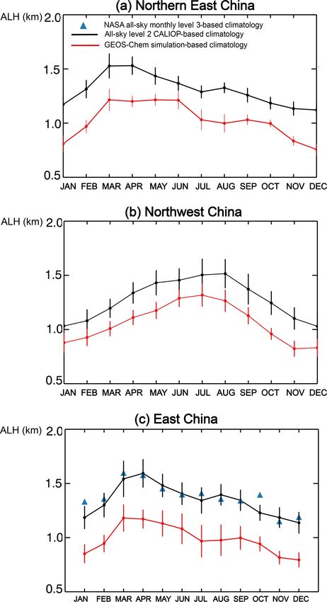
M. Liu et al.: OMI tropospheric NO2 retrieval over East Asia                                                                   3

of the same month in any year. We then use the corrected          tion spectroscopy (DOAS) technique (for the 405–465 nm
GEOS-Chem vertical extinction profiles in the retrievals of       spectral window in the case of OMI). The uncertainty of the
cloud parameters and NO2 . Finally, we evaluate our up-           SCD is determined by the appropriateness of the fitting tech-
dated POMINO retrieval (hereafter referred to as POMINO           nique, the instrument noise, the choice of fitting window, and
v1.1), our previous POMINO product, DOMINO v2, and the            the orthogonality of the absorbers’ cross sections (Bucsela et
newly released Quality Assurance for Essential Climate Vari-      al., 2006; Lerot et al., 2010; Richter et al., 2011; van Geffen
ables product (QA4ECV; see Appendix A), using ground-             et al., 2015; Zara et al., 2018). The NO2 SCD in DOMINO
based MAX-DOAS NO2 column measurements at three ur-               v2 has a bias at about 0.5–1.3 ×10¹⁵ molec. cm−2 (Dirksen
ban/suburban sites in East China for the year of 2012 and         et al., 2011; Belmonte Rivas et al., 2014; Marchenko et al.,
several months in 2008–2009.                                      2015; van Geffen et al., 2015; Zara et al., 2018), which can be
   Section 2 describes the construction of CALIOP aerosol         reduced by improving wavelength calibration and including
extinction vertical profile monthly climatology, the POMINO       O2 –O2 and liquid water absorption in the fitting model (van
v1.1 retrieval approach, and the MAX-DOAS data. It also           Geffen et al., 2015; Zara et al., 2018). The tropospheric SCD
presents the criteria for comparing different NO2 retrieval       is then obtained by subtracting the stratospheric SCD from
products and for selecting coincident OMI and MAX-DOAS            the total SCD. The bias in the total SCD is mostly absorbed
data. Section 3 compares our CALIOP climatology with              by this stratospheric separation step, which may not prop-
NASA’s official level 3 CALIOP dataset and GEOS-Chem              agate into the tropospheric SCD (van Geffen et al., 2015).
simulation results. Sections 4 and 5 compare POMINO v1.1          The last step converts the tropospheric SCD to VCD by us-
to POMINO to analyze the influence of improved aerosol            ing the tropospheric AMF (VCD = SCD/AMF). The tropo-
vertical profiles on retrievals of cloud parameters and NO2       spheric AMF is calculated at 438 nm by using look-up ta-
VCDs, respectively. Section 6 evaluates POMINO, POMINO            bles (in most retrieval algorithms) or online radiative trans-
v1.1, DOMINO v2, and QA4ECV NO2 VCD products using                fer modeling (in POMINO) driven by ancillary parameters,
the MAX-DOAS data. Section 7 concludes our study.                 which act as the dominant source of errors in retrieved NO2
                                                                  VCD data over polluted areas (Boersma et al., 2007; Lin et
                                                                  al., 2014b, 2015; Lorente et al., 2017).
2     Data and methods                                               Our POMINO algorithm focuses on the tropospheric
                                                                  AMF calculation over China and nearby regions, taking the
2.1    CALIOP monthly mean extinction profile
                                                                  tropospheric SCD (Dirksen et al., 2011) from DOMINO
       climatology
                                                                  v2 (Boersma et al., 2011). POMINO improves upon the
CALIOP is a dual-wavelength polarization lidar measuring          DOMINO v2 algorithm in the treatment of aerosols, surface
attenuated backscatter radiation at 532 and 1064 nm since         reflectance, online radiative transfer calculations, spatial
June 2006. The vertical resolution of aerosol extinction pro-     resolution of NO2 , temperature and pressure vertical pro-
files is 30 m below 8.2 km and 60 m up to 20.2 km (Winker et      files, and consistency between cloud and NO2 retrievals
al., 2013), with a total of 399 sampled altitudes. The horizon-   (Lin et al., 2014b, 2015). In brief, we use the parallelized
tal resolution of CALIOP scenes is 335 m along the orbital        LIDORT-driven AMFv6 package to derive both cloud
track and is given over a 5 km horizontal resolution in level 2   parameters and tropospheric NO2 AMFs for individual
data.                                                             OMI pixels online (rather than using a look-up table). NO2
   As detailed in Appendix B, we use the daily                    vertical profiles, aerosol optical properties, and aerosol
all-sky version 3 CALIOP level 2 aerosol profile                  vertical profiles are taken from the nested GEOS-Chem
product           (https://search.earthdata.nasa.gov/search?q=    model over Asia (0.667◦ long × 0.5◦ lat before May 2013
CALIOPaerosol&ok=CALIOP, last access: April 2017)                 and 0.3125◦ long × 0.25◦ lat afterwards), and pressure
aerosol at 532 nm from 2007 to 2015 to construct a monthly        and temperature profiles are taken from the GEOS-5-
level 3 climatological dataset of aerosol extinction profiles     and GEOS-FP-assimilated meteorological fields that drive
over China and nearby regions. This dataset is constructed        GEOS-Chem simulations. Model aerosols are further ad-
on the GEOS-Chem model grid (0.667◦ long × 0.5◦ lat) and          justed by satellite data (see below). We adjust the pressure
vertical resolution (47 layers, with 36 layers or so in the       profiles based on the difference in elevation between the
troposphere). The ratio of climatological monthly CALIOP          pixel center and the matching model grid cell (Zhou et al.,
to monthly GEOS-Chem profiles represents the scaling              2010). We also account for the effects of surface bidirec-
profile to adjust the daily GEOS-Chem profiles in the same        tional reflectance distribution function (BRDF) (Zhou et al.,
month (see Sect. 2.2)                                             2010; Lin et al., 2014b) by taking three kernel parameters
                                                                  (isotropic, volumetric, and geometric) from the MODIS
2.2    POMINO v1.1 retrieval approach                             MCD43C2         dataset     (https://search.earthdata.nasa.gov/
                                                                  search?q=MODISMCD43C2&ok=MODIS20MCD43C2,
The NO2 retrieval consists of three steps. First, the total       last access: December 2015) at 440 nm (Lucht et al., 2000).
NO2 SCD is retrieved using the differential optical absorp-

www.atmos-meas-tech.net/12/1/2019/                                                        Atmos. Meas. Tech., 12, 1–21, 2019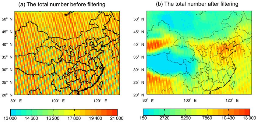
4                                                                   M. Liu et al.: OMI tropospheric NO2 retrieval over East Asia

   As a prerequisite to the POMINO NO2 retrieval, clouds are            2016) compiled on the model grid (Lin et al., 2014b, 2015).
retrieved through the O2 –O2 algorithm (Acarreta et al., 2004;          POMINO v1.1 uses the Collection 5.1 AOD data before
Stammes et al., 2008) with O2 –O2 SCDs from OMCLDO2,                    May 2013 and Collection 6 data afterwards. For adjust-
and with pressure, temperature, surface reflectance, aerosols,          ment, model AODs are projected to a 0.667◦ long × 0.5◦ lat
and other ancillary information consistent with the NO2 re-             grid and then sampled at times and locations with valid
trieval. Note that the treatment of cloud scattering (as an “ef-        MODIS data (Lin et al., 2015). As shown in Eq. (3), τ M de-
fective” Lambertian reflector, as in other NO2 algorithms) is           notes MODIS AOD, τ G GEOS-Chem AOD, and τ Mr post-
different from the treatment of aerosol scattering and absorp-          adjustment model AOD. The subscript i denotes a grid cell,
tion (vertically resolved based on the Mie scheme).                     d a day, m a month, and y a year. This AOD adjustment en-
   POMINO uses the temporally and spatially varying                     sures that in any month, monthly mean GEOS-Chem AOD
aerosol information, including AOD, SSA, phase func-                    is the same as MODIS AOD while the modeled day-to-day
tion, and vertical profiles from GEOS-Chem simulations.                 variability is kept.
POMINO v1.1 (this work) further uses CALIOP data to con-
                                                                                       M
                                                                                     τi,m,y
strain the shape of the aerosol vertical extinction profile. We           Gr                      G
                                                                        τi,d,m,y =            × τi,d,m,y                                 (3)
run the model at a resolution of 0.3125◦ long × 0.25◦ lat                              G
                                                                                     τi,m,y
before May 2013 and 0.667◦ long × 0.5◦ lat afterwards, as
determined by the resolution of the driving meteorological              Equations (4–5) show the complex effects of aerosols in cal-
fields. We then regrid the finer-resolution model results to            culating the AMF for any pixel. The AMF is the linear sum of
0.667◦ long × 0.5◦ lat, to be consistent with the CALIOP                tropospheric layer contributions to the slant column weighted
data grid. We then sample the model data at times and lo-               by the vertical sub-columns (Eq. 4). The box AMF, amfk ,
cations with valid CALIOP data at 532 nm to establish the               describes the sensitivity of NO2 SCD to layer k, and xa,k
model monthly climatology.                                              represent the sub-column of layer k from the a priori NO2
   For any month in a grid cell, we divide the CALIOP                   profile. The variable l represents the first integrated layer,
monthly climatology of aerosol extinction profile shape by              which is the layer above the ground for clear sky, or the layer
model climatological profile shape to obtain a unitless scal-           above cloud top for cloudy sky. The variable t represents the
ing profile (Eq. 1) and apply this scaling profile to all days of       tropopause layer. POMINO assumes the independent pixel
that month in all years (Eq. 2). Such a climatological adjust-          approximation (IPA) (Boersma et al., 2002; Martin, 2002).
ment is based on the assumption that systematic model lim-              This means that the calculated AMF for any pixel consists
itations are month dependent and persist over the years and             of a fully cloudy-sky portion (AMFclr ) and a fully clear-sky
days (e.g., a too strong vertical gradient; see Sect. 3.3). Al-         portion (AMFcld ), with weights based on the cloud radiance
                                                                                                 CF·Icld
though this monthly adjustment means discontinuity on the               fraction (CRF = (1−CF)·I                , where Iclr and Icld are ra-
                                                                                                   clr +CF·Icld
day-to-day basis (e.g., from the last day of a month to the             diance from the clear-sky part and fully cloudy part of the
first day of the next month), such discontinuity does not sig-          pixel, respectively) (Eq. 5). AMFcld is affected by above-
nificantly affect the NO2 retrieval, based on our sensitivity           cloud aerosols, and AMFclr is affected by aerosols in the en-
test.                                                                   tire column. Also, aerosols affect the retrieval of CRF. Thus,
   In Eqs. (1) and (2), E C represents the CALIOP climato-              the improvement of aerosol vertical profile in POMINO v1.1
logical aerosol extinction coefficient, E G the GEOS-Chem               affects all three quantities in Eq. (5) and thus leads to com-
extinction, E Gr the post-scaling model extinction, and R the           plex impacts on retrieved NO2 VCD.
scaling profile. The subscript i denotes a grid cell, k a ver-                    Pt
tical layer, d a day, m a month, and y a year. Note that in                          l amfk xa,k
                                                                        AMF = P         t                                                 (4)
Eq. (1), the extinction coefficient at each layer is normalized                         l xa,k
relative to the maximum value of that profile. This procedure           AMF = AMFcld · CRF + AMFclr · (1 − CRF)                          (5)
ensures that the scaling is based on the relative shape of the
extinction profile and is thus independent of the accuracies            2.3   OMI pixel selection to evaluate POMINO v1.1,
of CALIOP and GEOS-Chem AOD. We keep the absolute                             POMINO, DOMINO v2, and QA4ECV
AOD value of GEOS-Chem unchanged in this step.
            C           C                                               We exclude OMI pixels affected by row anomaly
           Ei,k,m /max(Ei,k,m )                                         (Schenkeveld et al., 2017) or with high albedo caused by
Ri,k,m =    G /max(E G )
                                                             (1)
           Ei,k,m   i,k,m                                               icy/snowy ground. To screen out cloudy scenes, we choose
 Gr           G                                                         pixels with a CRF below 50 % (effective cloud fraction is
Ei,k,d,m,y = Ei,k,d,m,y × Ri,k,m                             (2)
                                                                        typically below 20 %) in POMINO.
In POMINO, the GEOS-Chem AOD values are further                            The selection of CRF threshold influences the validity of
constrained by a MODIS/Aqua Collection 5.1 monthly                      pixels. The effective CRF in DOMINO implicitly includes
AOD dataset (https://search.earthdata.nasa.gov/search?q=                the influence of aerosols. In POMINO, the aerosol contri-
MODISAOD&ok=MODISAOD, last access: December                             bution is separated from that of the clouds, resulting in a

Atmos. Meas. Tech., 12, 1–21, 2019                                                                www.atmos-meas-tech.net/12/1/2019/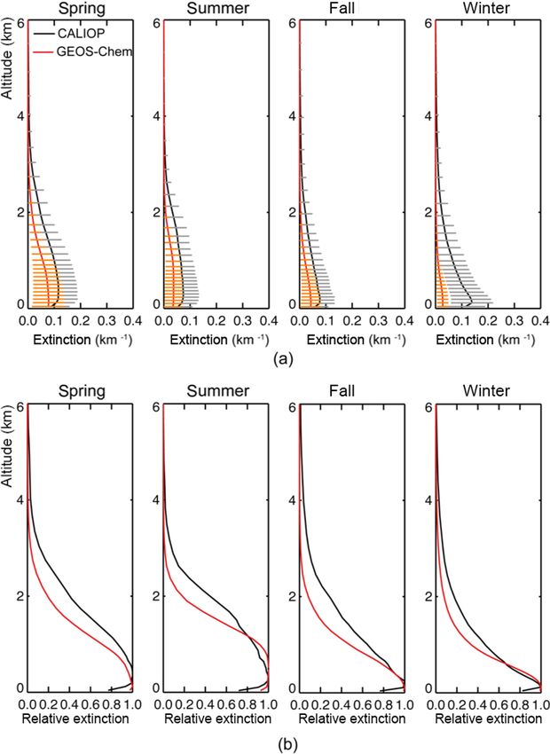
M. Liu et al.: OMI tropospheric NO2 retrieval over East Asia                                                                       5

Figure 1. (a) The three study areas include northern East China, northwest China, and East China. (b) MAX-DOAS measurement sites (red
dots) and corresponding meteorological stations (black triangle) overlaid on POMINO v1.1 NO2 VCDs in August 2012.

lower CRF than for DOMINO. The CRF differs insignif-                 by pollution from the surrounding major cities like Beijing
icantly between POMINO and POMINO v1.1 because the                   and Tianjin. At Xianghe, MAX-DOAS data have been con-
same AOD and other non-aerosol ancillary parameters are              tinuously available since early 2011, and data in 2012 are
used in the retrieval process. Using the CRF from POMINO             used here for comparison with OMI products. At IAP, MAX-
instead of DOMINO or QA4ECV for cloud screening means                DOAS data are available in 2008 and 2009 (Table 1); thus for
that the number of valid pixels in DOMINO increases by               comparison purposes we process OMI products to match the
about 25 %, particularly because many more pixels with high          MAX-DOAS times.
pollutant (aerosol and NO2 ) loadings are now included. This            Located on the roof of an 11-story building, the instru-
potentially reduces the sampling bias (Lin et al., 2014b,            ment at Wuxi was developed by the Anhui Institute of Optics
2015), and the ensemble of pixels now includes scenes with           and Fine Mechanics (AIOFM) (Wang et al., 2015, 2017a). Its
high “aerosol radiative fractions”. Further research is needed       telescope is pointed to the north and records at five elevation
to fully understand how much these high-aerosol scenes               angles (5, 10, 20, 30, and 90◦ ). Wuxi is a typical urban site
may be subject to the same screening issues as the cloudy            affected by heavy NOx and aerosol pollution. The measure-
scenes. Nevertheless, the limited evidence here and in Lin et        ments used here are analyzed in Wang et al. (2017a). Data
al. (2014b, 2015) suggests that including these high-aerosol         are available in 2012 for comparison with OMI products.
scenes does not affect the accuracy of NO2 retrieval.                   When comparing the four OMI products against MAX-
                                                                     DOAS observations, temporal and spatial inconsistency in
2.4   MAX-DOAS data                                                  sampling is inevitable. The spatial inconsistency, together
                                                                     with the substantial horizontal inhomogeneity in NO2 , might
We use MAX-DOAS measurements at three suburban or ur-                be more important than the influence of temporal inconsis-
ban sites in East China, including one urban site at the In-         tency (Wang et al., 2017b). The influence of the horizon-
stitute of Atmospheric Physics (IAP) in Beijing (116.38◦ E,          tal inhomogeneity was suggested to be about 10 %–30 % for
39.38◦ N), one suburban site in Xianghe County (116.96◦ E,           MAX-DOAS measurements in Beijing (Ma et al., 2013; Lin
39.75◦ N) to the south of Beijing, and one urban site in             et al., 2014b) and 10 %–15 % for less polluted locations like
Wuxi City (120.31◦ E, 31.57◦ N) in the Yangtze River Delta           Tai’an, Mangshan, and Rudong (Irie et al., 2012). Following
(YRD). Figure 1 shows the locations of these sites overlaid          previous studies, we average MAX-DOAS data within 1 h
with POMINO v1.1 NO2 VCDs in August 2012. Table 1                    of the OMI overpass time, and we select OMI pixels within
summarizes the information of MAX-DOAS measurements.                 25 km of a MAX-DOAS site whose viewing zenith angle is
   The instruments in IAP and in Xianghe were designed at            below 30◦ . To exclude local pollution events near the MAX-
BIRA-IASB (Clémer et al., 2010). Such an instrument is a             DOAS site (such as the abrupt increase in NO2 caused by
dual-channel system composed of two thermally regulated              the pass of consequent vehicles during a very short period),
grating spectrometers, covering the ultraviolet (300–390 nm)         the standard deviation of MAX-DOAS data within 1 h should
and visible (400–720 nm) wavelengths. It measures scattered          not exceed 20 % of their mean value (Lin et al., 2014b). We
sunlight every 15 min at nine elevation angles: 2, 4, 6, 8,          elect not to spatially average the OMI pixels because they
10, 12, 15, 30, and 90◦ . The telescope of the instrument is         can reflect the spatial variability in NO2 and aerosols.
pointed to the north. The data are analyzed following Hen-              We further exclude MAX-DOAS data in cloudy con-
drick et al. (2014). The Xianghe suburban site is influenced         ditions, as clouds can cause large uncertainties in MAX-

www.atmos-meas-tech.net/12/1/2019/                                                           Atmos. Meas. Tech., 12, 1–21, 2019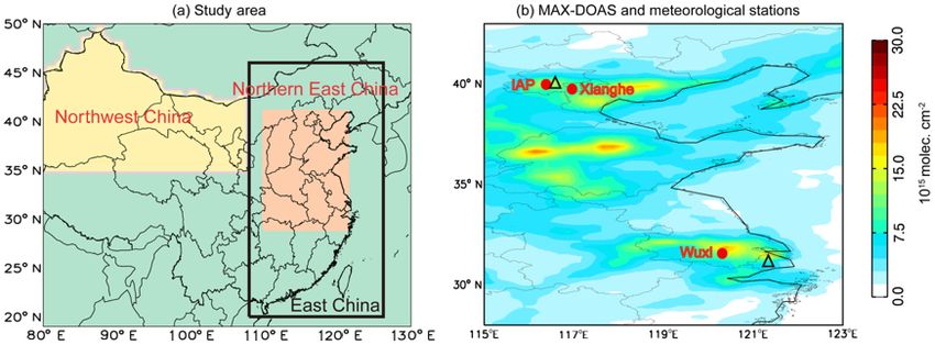
6                                                                 M. Liu et al.: OMI tropospheric NO2 retrieval over East Asia

Table 1. MAX-DOAS measurement sites and corresponding meteorological stations.

                      MAX-          Site               Measurement           Corresponding       Meteorological
                      DOAS par      information        times                 meteorological      station infor-
                      site name                                              station name        mation
                      Xianghe       116.96◦ E,         2012/01/01–           CAPITAL             116.89◦ E,
                                    39.75◦ N, 36 m,    2012/12/31            INTERNATIONA        40.01◦ N,
                                    suburban                                                     35.4 m
                      IAP           116.38◦ E,         2008/06/22–           CAPITAL             116.89◦ E,
                                    39.98◦ N, 92 m,    2009/04/16            INTERNATIONA        40.01◦ N,
                                    urban                                                        35.4 m
                      Wuxi          120.31◦ E,         2012/01/01–           HONGQIAO            121.34◦ E,
                                    31.57◦ N, 20 m,    2012/12/31            INTL                31.20◦ N,
                                    urban                                                        3m

DOAS and OMI data. To find the actual cloudy days, we                 3     Monthly climatology of aerosol extinction profiles
use MODIS/Aqua cloud fraction data, MODIS/Aqua level                        from CALIOP and GEOS-Chem
3 corrected reflectance (true color) data at 1◦ × 1◦ reso-
lution, and current weather data observed from the nearest            3.1    CALIOP monthly climatology
ground meteorological station (indicated by the black trian-
gles in Fig. 1b). Since there is only one meteorological sta-         The aerosol layer height (ALH) is a good indicator to what
tion available near the Beijing area, it is used for both IAP         extent aerosols are mixed vertically (Castellanos et al., 2015).
and Xianghe MAX-DOAS sites. We first use MODIS/Aqua                   As defined in Eq. A1 in Appendix B, the ALH is the average
corrected reflectance (true color) to distinguish clouds from         height of aerosols weighted by vertically resolved aerosol
haze. For cloudy days determined by the reflectance check-            extinction. Figure 2a shows the spatial distribution of our
ing, we examine both the MODIS/Aqua cloud fraction data               CALIOP ALH climatology in each season. At most places,
and the meteorological station cloud records, considering             the ALH reaches a maximum in spring or summer and a min-
that MODIS/Aqua cloud fraction data may be missing or                 imum in fall or winter. The lowest ALH in fall and winter can
have a too coarse of a horizontal resolution to accurately            be attributed to heavy near-surface pollution and weak verti-
interpret the cloud conditions at the MAX-DOAS site. We               cal transport. The high values in summer are related to strong
exclude MAX-DOAS NO2 data if the MODIS/Aqua cloud                     convective activities. Over the north, the high values in spring
fraction is larger than 60 % and the meteorological station re-       are partly associated with Asian dust events, due to high sur-
ports a “broken” (cloud fraction ranges from five-eighths to          face winds and dry soil in this season (Huang et al., 2010;
seven-eighths) or “overcast” (full cloud cover) sky. For the          Wang et al., 2010; Proestakis et al., 2018), which also affects
three MAX-DOAS sites together, this leads to 49 days with             the oceanic regions via atmospheric transport. The spring-
valid data out of 64 days with pre-screening data.                    time high ALH over the south may be related to the trans-
   We note here that using cloud fraction data from                   port of carbonaceous aerosols from Southeast Asian biomass
MODIS/Aqua or MAX-DOAS (for Xianghe only, see Gielen                  burning (Jethva et al., 2016). Averaged over the domain, the
et al., 2014) alone to screen cloudy scenes may not be appro-         seasonal mean ALHs are 1.48, 1.43, 1.27, and 1.18 km in
priate on heavy-haze days. For example, on 8 January 2012,            spring, summer, fall, and winter.
MODIS/Aqua cloud fraction is about 70 %–80 % over the                    Figure 3a, b further show the climatological monthly vari-
North China Plain and MAX-DOAS at Xianghe suggests the                ations in ALH averaged over northern East China (the an-
presence of thick clouds. However, both the meteorological            thropogenic source region shown in orange in Fig. 1a) and
station and MODIS/Aqua corrected reflectance (true color)             northwest China (the dust source region shown in yellow in
products suggest that the North China Plain was covered by            Fig. 1a). The two regions exhibit distinctive temporal vari-
a thick layer of haze. Consequently, this day was excluded            ations. Over northern East China, the ALH reaches a max-
from the analysis.                                                    imum in April (∼ 1.53 km) and a minimum in December
                                                                      (∼ 1.14 km). Over northwest China, the ALH peaks in Au-
                                                                      gust (∼ 1.59 km) because of the strongest convection (Zhu et
                                                                      al., 2013), although the springtime ALH is also high.
                                                                         Figure 4a shows the climatological seasonal regional aver-
                                                                      age vertical profiles of aerosol extinction over northern East
                                                                      China. Here, the aerosol extinction increases from the ground

Atmos. Meas. Tech., 12, 1–21, 2019                                                            www.atmos-meas-tech.net/12/1/2019/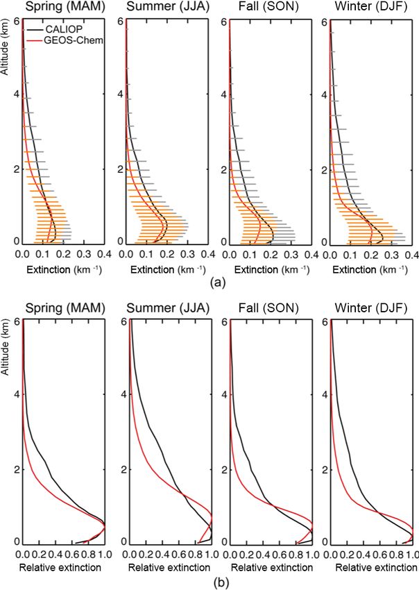
M. Liu et al.: OMI tropospheric NO2 retrieval over East Asia                                                                            7

Figure 2. Seasonal spatial patterns of ALH climatology at 532 nm on a 0.667◦ long × 0.50◦ lat grid based on (a) our compiled all-sky level
2 CALIOP data, (b) corresponding GEOS-Chem simulations, and (c) NASA all-sky monthly level 3 CALIOP dataset.

level to a peak at about 300–600 m (season dependent), above              Overall, the spatial and seasonal variations in CALIOP
which it decreases gradually. The height of peak extinction is         aerosol vertical profiles are consistent with changes in me-
lowest in winter, consistent with a stagnant atmosphere, thin          teorological conditions, anthropogenic sources, and natural
mixing layer, and increased emissions (from residential and            emissions. The data will be used to evaluate and adjust
industrial sectors). The large error bars (horizontal lines in         GEOS-Chem simulation results in Sect. 3.2. A comparison
different layers, standing for 1 standard deviation) indicate          of our CALIOP dataset with NASA’s official level 3 data is
strong spatiotemporal variability in aerosol extinction.               presented in Appendix C.
   Over northwest China (Fig. 5a), the column total aerosol
extinction is much smaller than that over northern East China
                                                                       3.2   Evaluation of GEOS-Chem aerosol extinction
(Fig. 4a), due to lower anthropogenic sources and dominant
                                                                             profiles
natural dust emissions. Vertically, the decline of extinction
from the peak-extinction height to 2 km is also much more
gradual than the decline over northern East China, indicat-            Figure 2b shows the spatial distribution of seasonal ALHs
ing stronger lifting of surface emitted aerosols. In winter, the       simulated by GEOS-Chem. The model captures the spa-
column total aerosol extinction is close to the high value in          tial and seasonal variations in CALIOP ALH (Fig. 2a) to
dusty spring, whereas the vertical gradient of extinction is           some degree, with an underestimate by about 0.3 km on aver-
strongest among the seasons. This reflects the high anthro-            age. The spatial correlation between CALIOP (Fig. 2a) and
pogenic emissions in parts of northwest China, which have              GEOS-Chem (Fig. 2b) ALH is 0.37 in spring, 0.57 in sum-
been rapidly increasing in the 2000s due to relatively weak            mer, 0.40 in fall, and 0.44 in winter. The spatiotemporal con-
emission control supplemented by growing activities of relo-           sistency and underestimate are also clear from the regional
cation of polluted industries from the eastern coastal regions         mean monthly ALH data in Fig. 3 – the temporal correlation
(Zhao et al., 2015; Cui et al., 2016).                                 between GEOS-Chem and CALIOP ALH is 0.90 in northern
                                                                       East China and 0.97 in northwest China.

www.atmos-meas-tech.net/12/1/2019/                                                               Atmos. Meas. Tech., 12, 1–21, 2019
8                                                                    M. Liu et al.: OMI tropospheric NO2 retrieval over East Asia

                                                                         Figure 4. (a) Seasonal climatological aerosol extinction profiles
                                                                         and (b) corresponding relative extinction profiles (normalized to
                                                                         maximum extinction values) in spring (MAM), summer (JJA),
Figure 3. Regional mean ALH monthly climatology over (a) north-          fall (SON), and winter (DJF) over northern East China. Model re-
ern East China, (b) northwest China, and (c) East China. The error       sults (in red) are prior to MODIS/Aqua-based AOD adjustment. Er-
bars stand for 1 standard deviation for spatial variability.             ror bars in (a) represent 1 standard deviation across all grid cells in
                                                                         each season.

                                                                            Since the POMINO v1.1 algorithm uses MODIS AOD to
   Figures 4a and 5a show the GEOS-Chem-simulated 2007–                  adjust model AOD, it only uses the CALIOP aerosol extinc-
2015 monthly climatological vertical profiles of aerosol ex-             tion profile shape to adjust the modeled shape (Eqs. 1 and 2).
tinction coefficient over northern East China and northwest              Figures 4a and 5b show the vertical shapes of aerosol extinc-
China, respectively. Over northern East China (Fig. 4a), the             tion, averaged across all profiles in each season over northern
model (red line) captures the vertical distribution of CALIOP            East China and northwest China, respectively. Over north-
extinction (black line) below the height of 1 km, despite a              ern East China (Fig. 4b), GEOS-Chem underestimates the
slight underestimate in the magnitude of extinction and an               CALIOP values above 1 km by 52 %–71 %. This underesti-
overestimate in the peak-extinction height. From 1 to 5 km               mate leads to a lower ALH, consistent with the finding by
above the ground, the model substantially overestimates the              van Donkelaar et al. (2013) and Lin et al. (2014b). Over
rate of decline in extinction coefficient with increasing al-            northwest China (Fig. 5b), the model also underestimates the
titude. Across the seasons, GEOS-Chem underestimates the                 CALIOP values above 1 km by 50 %–62 %. These results im-
magnitude of aerosol extinction by up to 37 % (depending                 ply the importance of correcting the modeled aerosol vertical
on the height). Over northwest China (Fig. 5a), GEOS-Chem                shape prior to cloud and NO2 retrievals.
has an underestimate in all seasons, with the largest bias by
about 80 % in winter likely due to underestimated water-
soluble aerosols and dust emissions (J. Wang et al., 2008;
Li et al., 2016).

Atmos. Meas. Tech., 12, 1–21, 2019                                                               www.atmos-meas-tech.net/12/1/2019/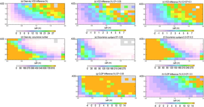
M. Liu et al.: OMI tropospheric NO2 retrieval over East Asia 9
Figure 6a, b show that over the two regions, the CTH
varies notably from one month to another, whereas the ALH
is much more stable across the months. Over northern East
China, the ALH increases by 0.52 km from POMINO (or-
ange dashed line) to POMINO v1.1 (orange solid line) due
to the CALIOP-based monthly climatological adjustment.
The increase in ALH means a stronger “shielding” effect of
aerosols on the O2 –O2 absorbing dimer, which, in turn, re-
sults in a reduced CTH by 0.69 km on average. For POMINO
over northern East China (Fig. 6a), the retrieved clouds usu-
ally extend above the aerosol layer, i.e., the CTH (grey
dashed line) is much larger than the ALH (orange dashed
line). Using the CALIOP climatology in POMINO v1.1 re-
sults in the ALH higher than the CTH in fall and winter. The
more elevated ALH is consistent with the finding of Jethva
et al. (2016) that a significant amount of absorbing aerosol
resides above clouds over northern East China based on 11-
year (2004–2015) OMI near-UV observations.
The CTH in northwest China is much lower than in north-
ern East China (Fig. 6a versus Fig. 7b). This is because the
dominant type of actual clouds is (optically thin) cirrus over
western China (Wang et al., 2014), which is interpreted by
the O2 –O2 cloud retrieval algorithm as reduced CTH (with
cloud base from the ground). The reduction in CTH from
POMINO to POMINO v1.1 over northwest China is also
smaller than the reduction over northern East China, albeit
with a similar enhancement in ALH, due to lower aerosol
loadings (Fig. 6c versus Fig. 6d).
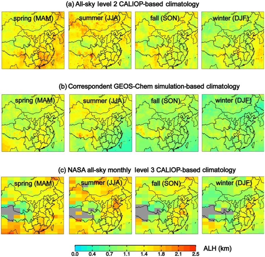
Figure 5. Similar to Fig. 4 but for northwest China. Figure 7g, h present the relative change in CP from
POMINO to POMINO v1.1 as a function of AOD (binned
at an interval of 0.1) and changes in ALH from POMINO to
POMINO v1.1 (1ALH, binned every 0.2 km) across all pix-
4 Effects of aerosol vertical profile improvement on els in 2012 over northern East China. Results are separated
cloud retrieval in 2012 for low cloud fraction (CF < 0.05 in POMINO, Fig. 7g) and
modest cloud fraction (0.2 < CF < 0.3, Fig. 7h). The median
Figure 6a, b show the monthly average ALH and cloud- of the CP changes for pixels within each AOD and 1ALH
top height (CTH, corresponding to cloud pressure, CP) over bin is shown. Figure 7e, f present the corresponding numbers
northern East China and northwest China in 2012. In order of occurrence under the two cloud conditions.
to discuss the CTH, only cloudy days are analyzed here, by Figure 7 shows that over northern East China, the increase
excluding days with zero cloud fraction (CF = 0, clear-sky in ALH is typically within 0.6 km for the case of CF < 0.05
cases) in POMINO. Although clear sky is used sometimes in (Fig. 7e), and the corresponding increase in CP is within
the literature to represent low cloud coverage (e.g., CF < 0.2 6 % (Fig. 7g). In this case, the average CTH (2.95 km in
or CRF < 0.5; Boersma et al., 2011; Chimot et al., 2016), POMINO versus 1.58 km in POMINO v1.1) becomes much
here it strictly means CF = 0 while cloudy sky means CF > 0. lower than the average ALH (1.06 km in POMINO versus
About 62.7 % of days contain non-zero fractions of clouds 1.98 km in POMINO v1.1). For the case with CF between 0.2
over northern East China, and the number is 59.1 % for north- and 0.3, the increase in ALH is within 1.2 km for most scenes
west China. The CF changes from POMINO to POMINO (Fig. 7f), which leads to a CP change of 2 % (Fig. 7h), much
v1.1 (i.e., after aerosol vertical profile adjustment) are negli- smaller than the CP change for CF < 0.05 (Fig. 7g). This is
gible (within ±0.5 %, not shown) due to the same values of partly because the larger the CF is, the smaller a change in
AOD and SSA used in both products. This is because overall CF is required to compensate for the 1ALH in the O2 –O2
CF is mostly driven by the continuum reflectance at 475 nm cloud retrieval algorithm. Furthermore, with 0.2 < CF < 0.3,
(mainly determined by AOD and surface reflectance, which the mean value of CTH is much higher than ALH in both
remain unchanged), which is insensitive to the aerosol pro- POMINO (2.76 km for CTH versus 1.13 km for ALH) and
file but CTH is driven by the O2 –O2 SCD, which is itself POMINO v1.1 (2.60 km for CTH versus 2.09 km for ALH);
impacted by ALH. thus a large portion of clouds are above aerosols so that the
www.atmos-meas-tech.net/12/1/2019/ Atmos. Meas. Tech., 12, 1–21, 2019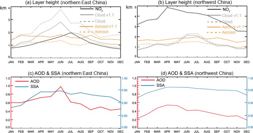
10                                                                  M. Liu et al.: OMI tropospheric NO2 retrieval over East Asia

Figure 6. Monthly variations in ALH, CTH, and NLH over (a) northern East China and (b) northwest China in 2012. Data are averaged
across all pixels in each month and region. The grey and orange solid lines denote POMINO v1.1 results, while the corresponding dashed
lines denote POMINO. (c–d) Corresponding monthly AOD and SSA.

Figure 7. Percentage changes in VCD from POMINO to POMINO v1.1 ([POMINO v1.1–POMINO]/POMINO) for each bin of 1ALH
(bin size = 0.2 km) and AOD (bin size = 0.1) across pixels in 2012 over northern East China, for (a) cloud-free sky (CF = 0 in POMINO),
(b) slightly cloudy sky, and (c) modestly cloudy sky. (d–f) The number of occurrences corresponding to (a–c). (g, h) Similar to (b, c) but for
the percentage changes in cloud-top pressure (CP).

change in CP is less sensitive to 1ALH. We find that the                   For northwest China (not shown), the dependence of CP
summertime data contribute the highest portion (36.5 %) to               changes on AOD and 1ALH is similar to that for northern
the occurrences for 0.2 < CF < 0.3.                                      East China. In particular, the CP change is within 10 % on

Atmos. Meas. Tech., 12, 1–21, 2019                                                               www.atmos-meas-tech.net/12/1/2019/
M. Liu et al.: OMI tropospheric NO2 retrieval over East Asia                                                                  11

Figure 8. Seasonal spatial distribution of tropospheric NO2 VCD in 2012 for (a) POMINO v1.1, (b) POMINO, and (c) their relative
difference.

average for the case of CF < 0.05 and 1.5 % for the case of       the optical effect of aerosols on tropospheric NO2 . Figure 6a
0.2 < CF < 0.3.                                                   presents the nitrogen layer height (NLH, defined as the aver-
                                                                  age height of model-simulated NO2 weighted by its volume
                                                                  mixing ratio in each layer) in comparison to the ALH and
5   Effects of aerosol vertical profile improvement on            height of the cloud layer top (CLH) over northern East China.
    NO2 retrieval in 2012                                         The figure shows that the POMINO v1.1 CTH is higher than
                                                                  the NLH in all months and higher than the ALH in warm
Figure 7a presents the percentage changes in clear-sky NO2        months, which means there is a shielding effect on both NO2
VCD from POMINO to POMINO v1.1 as a function of                   and aerosols.
binned AOD and 1ALH over northern East China. Here,                  Over northwest China (not shown), the changes in clear-
clear-sky pixels are chosen based on CF = 0 in POMINO.            sky NO2 VCD are within 9 % for most cases, which are much
In any AOD bin, an increase in 1ALH leads to an enhance-          smaller than over East China (within 18 %). This is because
ment in NO2 . And for any 1ALH, the change in VCD is              the NLH is much higher than the CLH and ALH (Fig. 6b) in
greater (smaller) when AOD becomes larger (smaller), which        absence of surface anthropogenic emissions.
indicates that the NO2 retrieval is more sensitive to ALH in         We convert the valid pixels into monthly mean level 3
high-aerosol-loading cases. Clearly, the change in NO2 is not     value datasets on a 0.25◦ long × 0.25◦ lat grid. Figure 8a, b
a linear function of AOD and 1ALH.                                compare the seasonal spatial variations in NO2 VCD in
   For cloudy scenes (Fig. 7b, c, cloud data are based on         POMINO v1.1 and POMINO in 2012. In both products, NO2
POMINO), the change in NO2 VCD is less sensitive to AOD           peaks in winter due to the longest lifetime and highest anthro-
and 1ALH. This is because the existence of clouds limits          pogenic emissions (Lin, 2012). NO2 also reaches a maximum

www.atmos-meas-tech.net/12/1/2019/                                                        Atmos. Meas. Tech., 12, 1–21, 2019
12 M. Liu et al.: OMI tropospheric NO2 retrieval over East Asia
Figure 9. (a–d) Scatter plot for NO2 VCDs (1015 molec. cm−2 ) between MAX-DOAS and each of the three OMI products. Each “+”
corresponds to an OMI pixel, as several pixels may be available in a day. (e–h) Similar to (a–d) but after averaging over all OMI pixels in the
same day, such that each “+” represents a day. Also shown are the statistic results from the RMA regression. The solid black line indicates
the regression curve and the grey dotted line depicts the 1 : 1 relationship.
over northern East China as a result of substantial anthro- els in a day are averaged (Fig. 9e, f), the correlation across
pogenic sources. From POMINO to POMINO v1.1, the NO2 the total of 49 days further increases for both POMINO v1.1
VCD increases by 3.4 % (−67.5 %–41.7 %) in spring for the (R 2 = 0.89) and POMINO (R 2 = 0.86), whereas POMINO
domain average (range), 3.0 % (−59.5 %–34.4 %) in sum- v1.1 still has a lower NMB (−3.7 %) and better slope (0.96)
mer, 4.6 % (−15.3 %–39.6 %) in fall, and 5.3 % (−68.4 %– than POMINO (−10.4 % and 0.82, respectively). These re-
49.3 %) in winter. The NO2 change is highly dependent on sults suggest that correcting aerosol vertical profiles, at least
the location and season. The increase over northern East on a climatology basis, already leads to a significantly im-
China is largest in winter, wherein the positive value for proved NO2 retrieval from OMI.
1ALH implies that elevated aerosol layers shield the NO2 Figure 9 shows that DOMINO v2 is correlated with
absorption. MAX-DOAS (R 2 = 0.68 in Fig. 9c and 0.75 in Fig. 9g)
but not as strong as POMINO and POMINO v1.1 for all
days. The discrepancy between DOMINO v2 and MAX-
6 Evaluating satellite products using MAX-DOAS data DOAS is particularly large for very high NO2 values (> 70 ×
1015 molec. cm−2 ). The R 2 for QA4ECV (0.75 in Fig. 9d
We use MAX-DOAS data, after cloud screening (Sect. 2.4), and 0.82 in Fig. 9h) is slightly better than DOMINO, but the
to evaluate DOMINO v2, QA4ECV, POMINO, and NMB is higher (−22.0 % and −22.7 %) and the slope drops
POMINO v1.1. The scatter plots in Fig. 9a–d compare the to 0.66. These results are consistent with the finding of Lin
NO2 VCDs from 162 OMI pixels on 49 days with their et al. (2014b, 2015) that explicitly including aerosol optical
MAX-DOAS counterparts. The statistical results are shown effects improves the NO2 retrieval.
in Table 2 as well. Different colors differentiate the seasons. Table 3 further shows the comparison statistics for 11
The high values of NO2 VCD (> 30 ×1015 molec. cm−2 ) oc- haze days. The haze days are determined when both the
cur mainly in fall (blue) and winter (black). POMINO v1.1 ground meteorological station data and MODIS/Aqua cor-
and POMINO capture the day-to-day variability in MAX- rected reflectance (true color) data indicate a haze day. The
DOAS data, i.e., R 2 = 0.80 for both products. The normal- table also lists AOD, SSA, CF, and MAX-DOAS NO2 VCD
ized mean bias (NMB) of POMINO v1.1 relative to MAX- as averaged over all haze days. A large amount of ab-
DOAS data (−3.4 %) is smaller than the NMB of POMINO sorbing aerosol occurs on these haze days (AOD = 1.13,
(−9.6 %). Also, the reduced major axis (RMA) regression SSA = 0.90). The average MAX-DOAS NO2 VCD reaches
shows that the slope for POMINO v1.1 (0.95) is closer to 51.9 × 10¹⁵ molec. cm−2 . Among the four satellite products,
unity than the slope for POMINO (0.78). When all OMI pix-
Atmos. Meas. Tech., 12, 1–21, 2019 www.atmos-meas-tech.net/12/1/2019/M. Liu et al.: OMI tropospheric NO2 retrieval over East Asia 13
Table 2. Pixel-based evaluation of OMI NO2 products with respect to MAX-DOAS for 162 pixels on 49 days.
POMINO v1.1 POMINO DOMINO v2 QA4ECV
Slope 0.95 0.78 1.06 0.66
Intercept (1015 molec. cm−2 ) −1.00 0.96 −3.86 1.09
R2 0.80 0.80 0.68 0.75
NMB (%) −3.4 −9.6 −2.1 −22.0
Table 3. Pixel-based evaluation of OMI NO2 products with respect to MAX-DOAS for 27 pixels on 11 haze daysa .
POMINO v1.1 POMINO DOMINO v2 QA4ECV
Slope 1.07 0.80 1.11 0.58
Intercept (1015 molec. cm−2 ) −3.58 1.76 −11.79 3.20
R2 0.76 0.68 0.38 0.34
NMB (%) 4.4 −9.4 −5.0 −26.1
a The haze days are determined when the ground meteorological station data and MODIS/Aqua corrected reflectance
(true color) data both indicate a haze day. Averages across the pixels are as follows: AOD = 1.13 (median = 1.10),
SSA = 0.90 (0.91), MAX-DOAS NO2 = 51.92 × 10¹⁵ molec. cm−2 , and CF = 0.06 (0.03).
POMINO v1.1 has the highest R 2 (0.76) and the lowest bias v1.1. Compared to monthly climatological CALIOP data
(4.4 %) with respect to MAX-DOAS, whereas DOMINO v2 over China, GEOS-Chem simulations tend to underestimate
and QA4ECV reproduce the variability to a limited extent the aerosol extinction above 1 km, as characterized by an un-
(R 2 = 0.38 and 0.34, respectively). This is consistent with derestimate in ALH by 300–600 m (seasonal and location
the previous finding that the accuracy of DOMINO v2 is re- dependent). Such a bias is corrected in POMINO v1.1 by
duced for polluted, aerosol-loaded scenes (Boersma et al., dividing, for any month and grid cell, the CALIOP monthly
2011; Kanaya et al., 2014; Lin et al., 2014b; Chimot et al., climatological profile by the model climatological profile to
2016). obtain a scaling profile and then applying the scaling profile
Table 4 shows the comparison statistics for 18 cloud- to model data on all days of that month in all years.
free days (CF = 0 in POMINO, and AOD = 0.60 on aver- The aerosol extinction profile correction leads to an in-
age). Here, POMINO v1.1, POMINO, and DOMINO v2 significant change in CF from POMINO to POMINO v1.1
do not show large differences in R 2 (0.53–0.56) and NMB since the AOD and surface reflectance are unchanged. In con-
(20.8 %–29.4 %) with respect to MAX-DOAS. QA4ECV has trast, the correction results in a notable increase in CP (i.e.,
a higher R 2 (0.63) and a lower NMB (−5.8 %), presum- a decrease in CTH), due to lifting of aerosol layers. The CP
ably reflecting the improvements in this (EU) consortium changes are generally within 6 % for scenes with a low cloud
approach, at least in mostly cloud-free situations. However, fraction (CF < 0.05 in POMINO) and within 2 % for scenes
the R 2 values for POMINO and POMINO v1.1 are much with a modest cloud fraction (0.2 < CF < 0.3 in POMINO).
smaller than the R 2 values on haze days, whereas the oppo- The NO2 VCDs increase from POMINO to POMINO v1.1
site changes are true for DOMINO v2 and QA4ECV. Thus, in most cases due to lifting of aerosol layers that enhances
for this limited set of data, the changes from DOMINO v2 the shielding of NO2 absorption. The NO2 VCD increases
and QA4ECV to POMINO and POMINO v1.1 mainly re- by 3.4 % (−67.5 %–41.7 %) in spring for the domain av-
flect the improved aerosol treatment in hazy scenes. Further erage (range), 3.0 % (−59.5 %–34.4 %) in summer, 4.6 %
research may use additional MAX-DOAS datasets to evalu- (−15.3 %–39.6 %) in fall, and 5.3 % (−68.4 %–49.3 %) in
ate the satellite products more systematically. winter. The NO2 changes are highly season and location de-
pendent and are most significant for wintertime in northern
East China.
7 Conclusions Further comparisons with independent MAX-DOAS NO2
VCD data for 162 OMI pixels on 49 days show good per-
This paper improves upon our previous POMINO algorithm formance of both POMINO v1.1 and POMINO in capturing
(Lin et al., 2015) to retrieve the tropospheric NO2 VCDs the day-to-day variation in NO2 (R 2 = 0.80, n = 162), com-
from OMI by compiling a 9-year (2007–2015) CALIOP pared to DOMINO v2 (R 2 = 0.67) and the new QA4ECV
monthly climatology of aerosol vertical extinction profiles to product (R 2 = 0.75). The NMB is smaller in POMINO v1.1
adjust GEOS-Chem aerosol profiles used in the NO2 retrieval (−3.4 %) than in POMINO (−9.6 %), with a slightly bet-
process. The improved algorithm is referred to as POMINO ter slope (0.804 versus 0.784). On hazy days with high
www.atmos-meas-tech.net/12/1/2019/ Atmos. Meas. Tech., 12, 1–21, 201914 M. Liu et al.: OMI tropospheric NO2 retrieval over East Asia
Table 4. Evaluation of OMI NO2 products with respect to MAX-DOAS of 36 pixels on 18 cloud-free daysa .
POMINO v1.1 POMINO DOMINO v2 QA4ECV
Slope 1.30 1.13 0.92 0.79
Intercept (1015 molec. cm −2 ) −0.61 0.31 2.32 1.05
R2 0.55 0.56 0.53 0.63
NMB (%) 29.4 20.8 21.9 −5.8
a CF = 0 in POMINO product. Averages across the pixels are as follows: AOD = 0.60 (median = 0.47), SSA = 0.90
(0.91), and MAX-DOAS NO2 = 26.82 × 10¹⁵ molec. cm−2 .
aerosol loadings (AOD = 1.13 on average), POMINO v1.1 Data availability. DOMINO v2 NO2 Level-2 data are available
has the highest R 2 (0.76) and the lowest bias (4.4 %) whereas at http://www.temis.nl/airpollution/no2col/data/omi/data_v2/
DOMINO and QA4ECV have difficulty in reproducing (European Space Agency, 2018); QA4ECV NO2 Level-2 data
the day-to-day variability in MAX-DOAS NO2 measure- at http://www.temis.nl/qa4ecv/no2col/data/omi/v1/ (European
ments (R 2 = 0.38 and 0.34, respectively). The four products Space Agency, 2018); and POMINO v2 NO2 Level-2 and
Level-3 data at https://www.amazon.com/clouddrive/share/
show small differences in R 2 on clear-sky days (CF = 0 in
zyC4mNEyRfRk0IX114sR51lWTMpcP1d4SwLVrW55iFG/
POMINO, AOD = 0.60 on average), among which QA4ECV
folder/S7IR7WSLSPikdLT_jsNX8g?_encoding=
shows the highest R 2 (0.63) and lowest NMB (−5.8 %), pre- UTF8&*Version*=1&*entries*=0&mgh=1 (ACM group at
sumably reflecting the improvements in less polluted places Peking University, 2018). POMINO NO2 v1.1 Level-2 data
such as Europe and the US. Thus the explicit aerosol treat- are available upon request. MODIS C5.1 AOD Level-2 data
ment (in POMINO and POMINO v1.1) and the aerosol ver- https://doi.org/10.1029/2006JD007815 (NASA Goddard Space
tical profile correction (in POMINO v1.1) improve the NO2 Flight, 2018); CALIOP v3 Level-2 aerosol extinction profile data
retrieval, especially in hazy cases. https://doi.org/10.1175/2010BAMS3009.1 (NASA Goddard Space
The POMINO v1.1 algorithm is a core step towards our Flight, 2018); CALIOP Level-3 aerosol extinction profile data
next public release of data product, POMINO v2. The v2 https://doi.org/10.5194/acp-13-3345-2013 (NASA Goddard Space
product will contain a few additional updates, including but Flight, 2018). MAX-DOAS data are available through contact with
the various data owners.
not limited to using MODIS Collection 6 merged 10 km
level 2 AOD data that combine the Dark Target (Levy et
al., 2013) and Deep Blue (Sayer et al., 2014) products, as
well as MODIS MCD43C2 Collection 6 daily BRDF data.
Meanwhile, the POMINO algorithm framework is being ap-
plied to the recently launched TROPOMI instrument that
provides NO2 information at a much higher spatial resolu-
tion (3.5 × 7 km2 ). A modified algorithm can also be used to
retrieve sulfur dioxide, formaldehyde, and other trace gases
from TROPOMI, for which purposes our algorithm will be
available to the community on a collaborative basis. Future
research can correct the SSA and NO2 vertical profile to fur-
ther improve the retrieval algorithm and can use more com-
prehensive independent data to evaluate the resulting satellite
products.
Atmos. Meas. Tech., 12, 1–21, 2019 www.atmos-meas-tech.net/12/1/2019/M. Liu et al.: OMI tropospheric NO2 retrieval over East Asia 15
Appendix A: Introduction to the QA4ECV product posphere). For each grid cell, we choose the CALIOP pixels
within 1.5◦ of the grid cell center. CALIOP level 2 data are
The QA4ECV NO2 product (http://www.qa4ecv.eu/, last ac- always presented at the fixed 399 altitudes above sea level.
cess: May 2018) builds on a (EU) consortium approach to To account for the difference in surface elevation between a
retrieve NO2 from GOME, SCIAMACHY, GOME-2, and CALIOP pixel and the respective model grid cell, we convert
OMI. The main contributions are provided by BIRA-IASB, the altitude of the pixel to a height above the ground, by us-
the University of Bremen (IUP), MPIC, KNMI, and Wa- ing the surface elevation data provided in CALIOP. We then
geningen University. Uncertainties in spectral fitting for NO2 horizontally and vertically average the profiles of all pixels
SCDs and in AMF calculations were evaluated by Zara et within one model grid cell and layer. We do the regridding
al. (2018) and Lorente et al. (2017), respectively. QA4ECV day by day for all grid cells to ensure that GEOS-Chem and
contains improved SCD NO2 data (Zara et al., 2018). Our CALIOP extinction profiles are coincident spatially and tem-
test suggests that using the QA4ECV SCD data instead of porally. Finally, we compile a monthly climatological dataset
DOMINO SCD data would reduce the underestimate against by averaging over 2007–2015.
MAX-DOAS VCD data from 3.7 % to 0.2 %, a relatively mi- Figure A1 shows the number of aerosol extinction pro-
nor improvement. Lorente et al. (2017) showed that across files in each grid cell and 12 × 9 = 108 months that are used
the above algorithms, there is a structural uncertainty by to compile the CALIOP climatology, both before and after
42 % in the NO2 AMF calculation over polluted areas. By data screening. Table A1 presents additional information on
comparing to our POMINO product, Lorente et al. also monthly and yearly bases. On average, there are 165 and 47
showed that the choice of aerosol correction may introduce aerosol extinction profiles per month per grid cell before and
an additional uncertainty by up to 50 % for situations with after screening, respectively. In the final 9-year monthly cli-
high polluted cases, consistent with Lin et al. (2014b, 2015) matology, each grid cell has about 420 aerosol extinction
and the findings here. For a complete description of the profiles on average, about 28 % of the prior-screening pro-
QA4ECV algorithm improvements, and quality assurance, files. Figure A1 shows that the number of valid profiles de-
please see Boersma et al. (2018). creases sharply over the Tibet Plateau and at higher latitudes
(> 43◦ N) due to complex terrain and icy/snowy ground.
As discussed above, we choose the CALIOP pixels within
Appendix B: Constructing the CALIOP monthly 1.5◦ of a grid cell center. We test this choice by examining the
climatology of aerosol extinction vertical profile ALH produced for that grid cell. The ALH is defined as the
extinction-weighted height of aerosols (see Eq. A1, where n
We use the all-sky level 2 CALIOP data to construct the level denotes the number of tropospheric layers, εi the aerosol ex-
3 monthly climatology. We choose the all-sky product in- tinction at layer i, and Hi the layer center height above the
stead of clear-sky data since previous studies indicate that ground). We find that choosing pixels within 1.0◦ of a grid
the climatological aerosol extinction profiles are affected in- cell center leads to a noisier horizontal distribution of ALH,
significantly by the presence of clouds (Koffi et al., 2012; owing to the small footprint of CALIOP. Conversely, choos-
Winker et al., 2013). As we use this climatological data to ing 2.0◦ leads to a too smooth spatial gradient of ALH with
adjust GEOS-Chem results, choosing all-sky data improves local characteristics of aerosol vertical distributions largely
consistency with the model simulation when doing the daily lost. We thus decide that 1.5◦ is a good balance between noise
correction. and smoothness.
To select valid pixels, we follow the data quality criteria by i=n
Winker et al. (2013) and Amiridis et al. (2015). Only the pix-
P
εi Hi
els with cloud–aerosol discrimination (CAD) scores between i=1
ALH = (B1)
−20 and −100 with an extinction quality control (QC) flag i=n
P
valued at 0, 1, 18, and 16 are selected. We further discard εi
i=1
samples with an extinction uncertainty of 99.9 km−1 , which
is indicative of unreliable retrieval. We only accept extinc- Certain grid cells do not contain sufficient valid observa-
tion values falling in the range from 0.0 to 1.25, according tions for some months of the climatological dataset. We fill
to CALIOP observation thresholds. Previous studies showed in missing monthly values of a grid cell using valid data in
that weakly scattering edges of icy clouds are sometimes the surrounding 5 × 5 = 25 grid cells (within ∼ 100 km). If
misclassified as aerosols (Winker et al., 2013). To eliminate the 25 grid cells do not have enough valid data, we use those
contamination from icy clouds we exclude the aerosol layers in the surrounding 7 × 7 = 49 grid cells (within ∼ 150 km).
above the cloud layer (with layer-top temperature below 0◦ ) A similar procedure is used by Lin et al. (2014b, 2015) to fill
when both of them are above 4 km (Winker et al., 2013). in missing values in the gridded MODIS AOD dataset.
After the pixel-based screening, we aggregate the For each grid cell in each month, we further correct singu-
CALIOP data at the model grid (0.667◦ long × 0.5◦ lat) and lar values in the vertical profile. In a month, if a grid cell i
vertical resolution (47 layers, with 36 layers or so in the tro- has an ALH outside mean ± 1σ of its surrounding 25 or 49
www.atmos-meas-tech.net/12/1/2019/ Atmos. Meas. Tech., 12, 1–21, 2019You can also read