Is deoxygenation detectable before warming in the thermocline?
←
→
Page content transcription
If your browser does not render page correctly, please read the page content below
Biogeosciences, 17, 1877–1895, 2020
https://doi.org/10.5194/bg-17-1877-2020
© Author(s) 2020. This work is distributed under
the Creative Commons Attribution 4.0 License.

Is deoxygenation detectable before warming in the thermocline?
Angélique Hameau1,2 , Thomas L. Frölicher1,2 , Juliette Mignot3 , and Fortunat Joos1,2
1 Climate
       and Environmental Physics, Physics Institute, University of Bern, Bern, Switzerland
2 Oeschger
        Centre for Climate Change Research, University of Bern, Bern, Switzerland
3 LOCEAN/IPSL, Sorbonne Université (SU)-CNRS-IRD-MNHN, Paris, France

Correspondence: Angélique Hameau (hameau@climate.unibe.ch)

Received: 27 August 2019 – Discussion started: 3 September 2019
Revised: 6 January 2020 – Accepted: 13 February 2020 – Published: 7 April 2020

Abstract. Anthropogenic greenhouse gas emissions cause           1   Introduction
ocean warming and oxygen depletion, with adverse impacts
on marine organisms and ecosystems. Warming is one of the
main indicators of anthropogenic climate change, but, in the     Carbon emissions from human activities are causing ocean
thermocline, changes in oxygen and other biogeochemical          warming (Rhein et al., 2013) and ocean deoxygenation,
tracers may emerge from the bounds of natural variability        i.e. a decrease in the oceanic oxygen (O2 ) concentration
prior to warming. Here, we assess the time of emergence          (Sarmiento et al., 1998; Bopp et al., 2002; Matear and Hirst,
(ToE) of anthropogenic change in thermocline temperature         2003; Battaglia and Joos, 2018). Both warming and deoxy-
and thermocline oxygen within an ensemble of Earth system        genation adversely affect marine organisms, ecosystems and
model simulations from the fifth phase of the Coupled Model      the services they provide (e.g. Pörtner et al., 2014; Deutsch
Intercomparison Project. Changes in temperature typically        et al., 2015; Gattuso et al., 2015; Magnan et al., 2016).
emerge from internal variability prior to changes in oxygen.        All major ocean basins have experienced significant
However, in about a third (35 ± 11 %) of the global thermo-      warming over the last few decades. Warming is generally
cline deoxygenation emerges prior to warming. In these re-       strongest at the surface and weaker at deeper layers, indica-
gions, both reduced ventilation and reduced solubility add to    tive of heat penetrating from the surface towards the deep
the oxygen decline. In addition, reduced ventilation slows the   ocean as expected from atmospheric greenhouse gas forc-
propagation of anthropogenic warming from the surface into       ing. The strongest warming in the top 2000 m has been ob-
the ocean interior, further contributing to the delayed emer-    served in the Southern Ocean (Roemmich et al., 2015) and
gence of warming compared to deoxygenation. Magnitudes           the tropical/subtropical Pacific and Atlantic Ocean (Cheng
of internal variability and of anthropogenic change, which       et al., 2017). On regional to local scales, the anthropogenic
determine ToE, vary considerably among models leading to         warming signal may be masked by natural interannual to
model–model differences in ToE. We introduce a new met-          multi-decadal variability. For example, decadal-scale cool-
ric, relative ToE, to facilitate the multi-model assessment of   ing trends in the tropical Pacific and Indian oceans may
ToE. This reduces the inter-model spread compared to the         arise from natural El Niño–Southern Oscillation and/or In-
traditionally evaluated absolute ToE. Our results underline      dian Ocean dipole variability (Han et al., 2014). Similarly,
the importance of an ocean biogeochemical observing sys-         decadal variability in the Atlantic meridional overturning is
tem and that the detection of anthropogenic impacts becomes      observed to modulate temperature and heat content change
more likely when using multi-tracer observations.                in the North Atlantic (Chen and Tung, 2018).
                                                                    Observation-based studies indicate that the global ocean
                                                                 oxygen content has decreased since 1960 (e.g. Schmidtko
                                                                 et al., 2017). Increased ocean surface temperature reduces
                                                                 oxygen solubility, limiting atmospheric oxygen dissolution
                                                                 into the upper ocean. In subsurface waters, oxygen concen-
                                                                 tration is also affected by changes in ventilation and the rem-

Published by Copernicus Publications on behalf of the European Geosciences Union.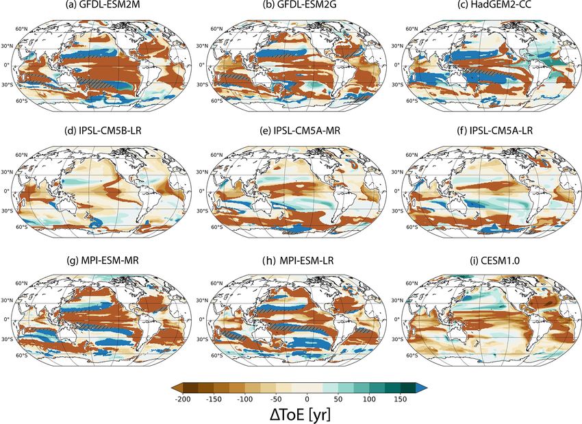
1878                                                          A. Hameau et al.: Is deoxygenation detectable before warming?

ineralisation of organic matter. In the contemporary ocean,         and pCO2 emerge earlier than sea surface temperature and
oxygen decreases in the interior are mostly dominated by            O2 change earlier than productivity. Changes in surface O2
a reduction in ventilation with a smaller role for changes          are tightly coupled to temperature-driven solubility changes
related to the production of organic matter, O2 solubility          and O2 varies hand in hand with sea surface temperature and
and air–sea equilibration of O2 in surface waters (Bopp             the two signals emerge typically concomitantly. Regarding
et al., 2002, 2017; Plattner et al., 2002; Tjiputra et al., 2018;   the ocean interior, the sequence of emergence for O2 and T
Hameau et al., 2019). The largest oxygen declines are located       is less clear. Global warming increases surface ocean tem-
in the Pacific Ocean (Equator and Northern Hemisphere) and          perature, which tends to reduce O2 . However, O2 is also in-
the Southern Ocean. However, observations are relatively            fluenced by non-thermal processes, such as respiration and
sparse and only start in the second half of the 20th cen-           the redistribution by ocean circulation and mixing. Respi-
tury. Therefore, it is challenging to distinguish human-caused      ration of organic matter in the ocean interior may have a
trends from natural variations in the observational record of       larger influence on O2 change than temperature-driven sol-
ocean O2 .                                                          ubility change in a more stratified and less ventilated ocean.
   Global climate models, such as the Earth system models           One could therefore expect that, under global warming, the
that participated in phase 5 of the Coupled Model Intercom-         combined effect of increased O2 consumption and decreased
parison Project (CMIP5), reproduce the long-term trend in           O2 solubility will accelerate the O2 depletion in subsurface
global ocean heat content over the last 50 years when uncer-        waters and that O2 may be detectable before the warming
tainties of observation-based estimates and internally gener-       reaches that layer.
ated natural variability are taken into account (Frölicher and         The concept of time of emergence (ToE; Christensen et al.,
Paynter, 2015; Cheng et al., 2019). Modelling studies agree         2007; Hawkins and Sutton, 2012) is often used to determine
on the sign of oceanic O2 changes but likely underestimate          the point in time when the anthropogenic signal becomes
the magnitude of loss (Bopp et al., 2013; Cocco et al., 2013;       larger than the range of natural variability. ToE has been
Oschlies et al., 2017). In particular in the tropical regions,      broadly used in climate change detection for physical cli-
models are not able to reproduce observed O2 decrease in            mate variables (e.g. surface temperature: Hawkins and Sut-
equatorial low-oxygen zones (Stramma et al., 2008; Cocco            ton, 2012; Frame et al., 2017), land carbon fluxes (Lom-
et al., 2013; Cabré et al., 2015).                                  bardozzi et al., 2014) or marine biogeochemical variables
   It is expected that ocean warming and deoxygenation, and         (e.g. pH, alkalinity, dissolved inorganic carbon (DIC), pCO2 :
the combination thereof, increase the risk of adverse impacts       Hauri et al., 2013; Keller et al., 2014; marine biological pro-
on marine organisms and ecosystem services (Pörtner et al.,         ductivity: Henson et al., 2016). A limited number of studies
2014). Warming of the ocean influences the physiology and           addressed anthropogenic deoxygenation detection in the sub-
ecology of almost all marine organisms. Reduced oceanic             surface layers (Rodgers et al., 2015; Frölicher et al., 2016;
O2 concentrations can disrupt marine ecosystems by push-            Henson et al., 2016, 2017; Long et al., 2016; Hameau et al.,
ing organisms to their species-specific limits of hypoxic tol-      2019). One study, Hameau et al. (2019), uses a single model
erance, below which the species are no longer able to meet          (Community Earth System Model; CESM), to investigate
their metabolic O2 demand. The species-specific metabolic           ToE of temperature and oxygen in the thermocline, find-
demand of O2 is also a function of temperature, as warmer           ing that anthropogenic ocean warming emerges much ear-
temperatures increase metabolic rates and oxygen require-           lier than the O2 signal in low-latitude and midlatitude re-
ments (Deutsch et al., 2015). At the same time, higher ocean        gions. Delayed emergence of changes in O2 is due to the
temperatures also decrease oxygen supply through reduced            opposing effects of O2 solubility and O2 consumption. In
ventilation, enlarging the regions with limited O2 concentra-       the high latitudes and the Pacific subtropical gyres, deoxy-
tions and thus shifting ecosystem distribution (Cheung et al.,      genation emerges before ocean warming in CESM. This oc-
2011).                                                              curs because decreases in oxygen solubility are reinforced
   Beyond the combined impact of physical and biogeo-               by increased O2 consumption, leading to strong O2 deple-
chemical changes, an interesting question is whether anthro-        tion. However, it is unknown if this single-model result is
pogenic changes in the ocean interior are first detectable in       robust across a suite of different Earth system model simula-
variables that are routinely and frequently measured such           tions. Here, we conduct a multi-model study to more broadly
as temperature (T ) or in variables with a relatively low ob-       test the hypothesis that anthropogenic deoxygenation in the
servational coverage but potentially high impact for ecosys-        thermocline emerges prior to anthropogenic warming. Since
tems such as O2 (Joos et al., 2003). The answer may have            the primary objective is to test the consistency across models
implications for measurement strategies to detect anthro-           of the order of emergence (deoxygenation prior to warming)
pogenic changes in subsurface waters as well as for the im-         within a single model, we introduce a relative ToE to conduct
pacts of physical and biogeochemical change on marine life.         the intercomparison, rather than the absolute year of ToE. We
For the surface ocean, earlier studies (Keller et al., 2014;        define relative ToE as a deviation relative to the model mean
Rodgers et al., 2015; Frölicher et al., 2016; Schlunegger           ToE for improved model intercomparison.
et al., 2019) showed that the anthropogenic signals of pH

Biogeosciences, 17, 1877–1895, 2020                                                     www.biogeosciences.net/17/1877/2020/
A. Hameau et al.: Is deoxygenation detectable before warming?                                                                 1879

   In this study, we analyse and compare the relative ToE(T )     drift in the control simulations is relatively small in the ther-
and ToE(O2 ) in the thermocline (200–600 m) using nine dif-       mocline (3.6±2.4×10⁻³ mmol m−3 yr−1 for trend in global
ferent CMIP5 Earth system models. We also assess the im-          mean oxygen concentration and 7.2 ± 6.6 × 10⁻⁵ ◦ C yr−1
pact of using the relative ToE in comparison to the clas-         for trend in global mean temperature averaged over 200–
sical approach using absolute ToE. In addition, we discuss        600 m), we detrended all model output with a linear trend ob-
the magnitude of background internal variability and anthro-      tained from the preindustrial control simulation in each grid
pogenic signal, and their translation into ToE. Finally, we       cell. The CESM1.0 simulation also shows some model drift.
analyse the role of solubility, ventilation and respiration for   Therefore, an exponential curve was fitted to the annual out-
the emergence of anthropogenic changes in oxygen and tem-         put of its associated control simulation at each grid cell. The
perature.                                                         detrending procedure is described in detail in Hameau et al.
                                                                  (2019).

2     Method                                                      2.2     Multi-model analysis methods

2.1    Earth system models                                        We use the concept of ToE (e.g. Hawkins and Sutton, 2012)
                                                                  to compare anthropogenic changes in O2 and temperature
We use output from eight different configurations of four         (signal; S) with internal variations (background noise; N).
Earth system models (ESMs) that participated in CMIP5             Here, ToE represents the moment in time at which the ocean
(Taylor et al., 2012): GFDL-ESM2M, GFDL-ESM2G,                    state becomes distinct from the preindustrial state. Appendix
HadGEM2-CC, IPSL-CM5A-LR, IPSL-CM5A-MR, IPSL-                     Fig. A1 provides a graphical illustration of the method used
CM5B-LR, MPI-ESM-LR and MPI-ESM-MR (Table 1). In                  to compute ToE.
order to extend the multi-model ensemble from four to five           We define the absolute ToE as the first year when the an-
family models, we also included the output from simula-           thropogenic signal S becomes equal to or larger than twice
tions performed with CESM1.0 conducted at the Swiss Su-           the noise of internal variability N (Eq. 1; following Hameau
percomputing Centre. The horizontal ocean model resolution        et al., 2019; Fig. A1). The threshold is set to 2 in order to dis-
is about 1° in both the Geophysical Fluid Dynamics Labora-        tinguish the signal from the noise at 95 % confidence level.
tory (GFDL) models and CESM1.0. Hadley Centre Global              Annual O2 and T data are first averaged over the thermocline
Environment Model version 2 – Carbon Cycle (HadGEM2-              (200–600 m) at each grid point of the horizontal grid, and lo-
CC) and Institut Pierre Simon Laplace (IPSL) models have a        cal S and N are computed from these depth-averaged values
horizontal resolution of about 2° and the MPI models have         for each model, variable and (horizontal) grid point. Annual
a horizontal resolution of about 0.4° (medium resolution;         anomalies are calculated relative to the preindustrial period
MR) and 1.5° (low resolution; LR). Of the nine models, all        (1860–1959).
but one (GFDL-ESM2G, isopycnal vertical coordinate) use
a pressure-based vertical coordinate. For additional informa-             S
                                                                  ToE :     >2                                                  (1)
tion on the individual model setups, the reader is referred to            N
the references listed in Table 1.
   Both the CMIP5 ESMs and the CESM1.0 were run un-                  The background noise, N, is computed as 1 standard devi-
der prescribed anthropogenic and natural greenhouse gas and       ation (SD) of O2 and of T from the annual preindustrial con-
aerosol forcing. All simulations span the historical 1861–        trol output. The entire duration of the control simulation is
2005 period and the 2006–2100 period following the Repre-         considered for each model to estimate the background noise.
sentative Concentration Pathway 8.5 (RCP8.5) scenario. The           N represents the noise due to the internal chaotic variabil-
RCP8.5 represents a high emission scenario with a radiative       ity of the climate system. Note that this definition of the noise
forcing of 8.5 W m−2 in the year 2100 (Riahi et al., 2011).       differs from Hameau et al. (2019), who used internal plus
These simulations are complemented with output from cor-          externally forced natural variability from a last-millennium
responding control runs with constant preindustrial forcing.      simulation to assess the standard background noise.
The CESM1.0 simulations differ from the CMIP5 simula-                The annual output of the forced, transient simulation
tions only with regard to the spin-up procedure. The CMIP5        (1860–2099) is smoothed by a low-pass spline filter (Enting,
model simulations are branched off from preindustrial con-        1987) to estimate S for each (horizontal) grid point in the
trol simulations, whereas the CESM1.0 simulation is an ex-        thermocline. The cut-off period of the spline is set to 80 years
tension of a last-millennium simulation run under 850 CE          to remove decadal to multi-decadal variations (e.g. associ-
conditions (Lehner et al., 2015). For this study, all CMIP5       ated with internal variability). The signal S is then defined as
models are used for which the three-dimensional output of         the value of the spline at each point in time.
oxygen, temperature and salinity for all simulations was             To ensure that S indeed detects anthropogenic trends, we
available on the Earth System Grid. We regridded all model        also apply a criterion for the sign of S to define ToE: S
output onto a regular 1◦ × 1◦ grid. Even though the model         needs to have the same sign as the difference between the

www.biogeosciences.net/17/1877/2020/                                                      Biogeosciences, 17, 1877–1895, 2020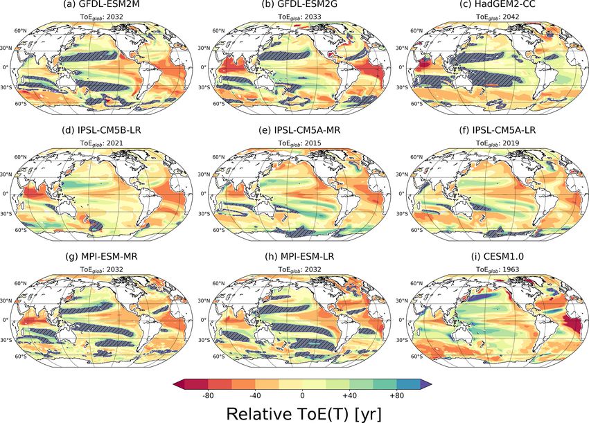
1880                                                             A. Hameau et al.: Is deoxygenation detectable before warming?

Table 1. Overview of the Earth system models used in this study, their configurations and vertical and approximated horizontal resolutions.

  Earth system model            Physical                               Biogeochemical                         Vertical and horizontal
                                ocean model                            ocean model                            ocean resolution
  CESM1.0                       POP2 (Smith et al., 2010;              BEC (Moore et al., 2002, 2004)         60 levels
  (Hurrell et al., 2013)        Danabasoglu et al., 2011)                                                     ∼ 1◦ × 1◦
  GFDL-ESM2M                    MOM4p1 (Griffies et al., 2011)                                                50 levels
                                                                       TOPAZ2 (Dunne et al., 2013)
  GFDL-ESM2G                    GOLD (Hallberg, 1997)                                                         ∼ 1◦ × 1◦
  (Dunne et al., 2012, 2013)
  HadGEM2-CC                    HadGEM2                                HadOCC (Palmer and Totterdell, 2001)   40 levels
  (Collins et al., 2011)        (Collins et al., 2011)                                                        ∼ 2◦ × 2◦
  IPSL-CM5A-LR                                                                                                31 levels
  IPSL-CM5A-MR                                                                                                ∼ 2◦ × 2◦
                                OPA (Madec et al., 2017)               PISCES (Aumont and Bopp, 2006)
  IPSL-CM5B-LR
  (Dufresne et al., 2013)
  MPI-ESM-LR                                                                                                  40 levels ∼ 1.5◦ × 1.5◦
                                MPIOM (Jungclaus et al., 2013)         HAMOCC5.2 (Ilyina et al., 2013)
  MPI-ESM-MR                                                                                                  40 levels ∼ 0.4◦ × 0.4◦
  (Giorgetta et al., 2013)

last 30 years of the future simulation and the preindustrial               2.3   Separating mechanisms of oxygen change
average for the corresponding variable and grid point.
   In order to minimise inter-model differences and to high-               To diagnose processes driving the simulated changes in
light the common spatial patterns of ToE, we introduce a new               ocean O2 , the direct thermal/solubility component of change
metric, the relative ToE (ToErel ). It is defined as the absolute          (O2,sol ) can be isolated from the total O2 change. The resid-
ToE (ToEabs ) minus the global area-averaged ToE (ToEglob ;                ual, apparent oxygen utilisation (AOU), represents the sum-
Eq. 2).                                                                    mation of all non-thermal changes, including those resulting
                                                                           from changes in ventilation and remineralisation.
ToErel = ToEabs − ToEglob                                        (2)
                                                                           [O2 ] = [O2,sol ] + [-AOU]                                   (3)
   S, N, ToE and ToErel are first computed from the an-
nual output for each model and at each (horizontal) grid                   The solubility component for each model is computed fol-
cell. Then, multi-model median and spread (interquartile                   lowing Garcia and Gordon (1992), which requires local salin-
range) of the multi-model estimations are computed from                    ity and temperature output. The solubility depends mostly on
the model ensemble. The median represents a “best” esti-                   temperature with a small contribution of salinity. The non-
mate and the interquartile range a measure of model un-                    thermal component ([-AOU]) is deduced from the difference
certainty. Uniform weights are applied to each model con-                  between O2,sol and O2 following Eq. (3). In Sect. 3.4, we
figuration to compute those statistics. Tests have been per-               will use changes in [-AOU] as a proxy for changes in water
formed using a weighted median as several simulations                      mass age and ventilation. Output of an ideal age tracer is not
stem from the same model family (CESM × 1; GFDL × 0.5;                     available for most models. A decrease in water exchange be-
HadGEM2 × 1; IPSL × 0.3; MPI × 0.5). However, the me-                      tween the surface ocean and the thermocline typically leads
dian and interquartile range of the multi-model ensemble are               to an increase in water mass age in the thermocline. There-
not sensitive to the weighting scheme applied (not shown).                 fore, changes in ventilation affect the balance between the
Because an anthropogenic signal may not emerge before the                  rate of supply of O2 -rich waters from the surface and the rate
end of the simulation in the year 2100, ToE can be unde-                   of O2 consumption by remineralisation of organic matter. It
fined. We therefore require that ToE values are defined for at             has been demonstrated in earlier studies (e.g. Gnanadesikan
least seven out of nine models to compute the multi-model                  et al., 2012; Bopp et al., 2017; Hameau et al., 2019) that a
statistics (median and spread). If more than two models have               decrease in [-AOU] typically corresponds to a decrease in
an undefined ToE, we mask the grid points in maps of the                   ventilation and an increase in water mass age, as simulated
multi-model median and of the multi-model spread.                          changes in the remineralisation rates of organic material and
                                                                           in associated O2 consumption are relatively small over the
                                                                           21st century.

Biogeosciences, 17, 1877–1895, 2020                                                             www.biogeosciences.net/17/1877/2020/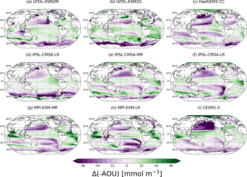
A. Hameau et al.: Is deoxygenation detectable before warming?                                                                       1881

Figure 1. Multi-model median (a, d) and spread (b, e) of relative ToE for temperature (a, b, c) and dissolved oxygen (d, e, f) for the
thermocline (200–600 m). The spread is computed as the interquartile range. Difference (c, f) between the multi-model spread of absolute
ToE estimates with the multi-model spread of relative ToE estimates for (c) temperature and (f) dissolved oxygen. The hatched areas show
regions with no emergence for at least three models. The relative ToE estimates are shown for each model in Figs. 2 and 3 and the absolute
estimates in Figs. S1 and S2 in the Supplement.

3     Results                                                          3.1.1   Anthropogenic warming

3.1    Relative time of emergence                                      ToErel (T ) shows early emergence in low latitudes and be-
                                                                       tween 30 and 60◦ S, and late emergence in the western trop-
We start by discussing the multi-model median and spread of            ical Pacific, in the Atlantic subpolar gyre and the subtropical
relative ToE estimates for potential temperature (Fig. 1a, b)          gyres of the Indian and Pacific oceans (Fig. 1a). The north-
and dissolved oxygen (Fig. 1d, e) changes in the thermocline           ern Indian Ocean and the eastern equatorial Atlantic stand
(200–600 m). An analysis of the roles of internal variabil-            out as the regions with earliest emergence in anthropogenic
ity and anthropogenic change ToE and why anthropogenic                 warming, i.e. 70 years (median of nine ToErel (T )) before the
change is detectable early or late is presented in Sect. 3.3.          global average ToE. No emergence of warming by the end of
                                                                       the 21st century (for at least three models; see Sect. 2.2) is

www.biogeosciences.net/17/1877/2020/                                                            Biogeosciences, 17, 1877–1895, 2020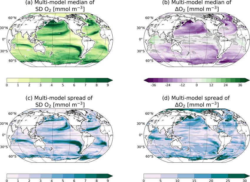
1882                                                           A. Hameau et al.: Is deoxygenation detectable before warming?

Figure 2. ToE of T in the thermocline (200–600 m) relative to the averaged ToE in that layer for each simulation. The hatched areas show
regions with no emergence by the end of the 21st century. The values of the global average ToE, ToEglob , are given above each panel. The
absolute ToE estimates are shown in Fig. S1.

simulated in the subtropical gyres of the Indian and Pacific              ToE values for individual horizontal grid cells are glob-
oceans, south of Greenland and locally south of 60◦ S.                 ally averaged to obtain an area-weighted global mean ToE for
   The multi-model spread in ToErel (T ) is generally small            the thermocline and each model. These global mean values
in regions with early emergence (Fig. 1b). This is the case            range between the years 1963 and 2033 for the nine models
in many regions of the Pacific and the Southern Ocean                  (see subtitles in Fig. 2). The patterns of ToErel (T ) for each
(±15 years). However, in the Atlantic subtropical gyres and            individual model are shown in Fig. 2. As described previ-
in the Arabian Sea, the early ToErel (T ) estimates are associ-        ously, low-latitude regions and parts of the Southern Ocean
ated with a wider spread across models (±25 to ±45 years).             show earlier emergence compared to mid- and other high-
Large inter-model spread is also found in the Kuroshio ex-             latitude regions. The HadGEM2-CC model (Fig. 2c) is an
tension and in the Indian and Atlantic region of the Southern          exception in that respect as temperature emerges later (+30
Ocean (±50 years). These regional differences in the multi-            to +50 years) than the global average in the tropical Atlantic
model spread could not be explained by the multi-model me-             and Pacific. In the Pacific and Indian subtropical gyre re-
dian of ToE, the anthropogenic signal nor the internal vari-           gions, the models show late (IPSL family) or no emergence.
ability amplitude for both O2 and T . Scatter plots of indi-           And finally, CESM and the IPSL family models are the only
vidual grid cell values of the multi-model spread in ToErel            models that show emergence before the end of the 21st cen-
versus those of the multi-model median of ToE, the anthro-             tury in the subtropical gyres of the Pacific.
pogenic signal or the internal variability amplitude do not
show a clear relationship (not shown). On average, the multi-
model spread for ToErel (T ) is about 25 years.

Biogeosciences, 17, 1877–1895, 2020                                                         www.biogeosciences.net/17/1877/2020/
A. Hameau et al.: Is deoxygenation detectable before warming? 1883
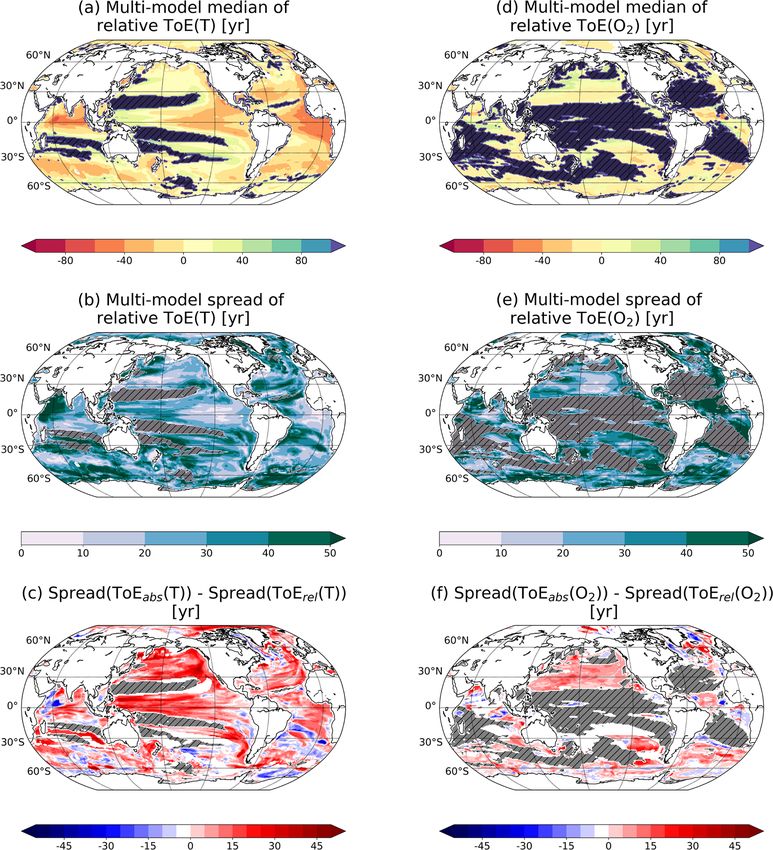
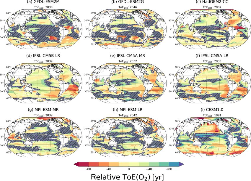
Figure 3. ToE of O2 in the thermocline (200–600 m) relative to the averaged ToE in that layer for each simulation. The hatched areas show
regions with no emergence by the end of the 21st century. The absolute ToE estimates are shown in Fig. S2. The global average ToE, ToEglob ,
is shown for each model.
3.1.2 Anthropogenic deoxygenation the eastern tropical Atlantic, the spread for ToErel (O2 ) is, de-
spite a smaller global mean spread, larger than for ToErel (T ).
In summary, even though the median pattern of ToErel (O2 ) is
In contrast to ToErel (T ), most of the thermocline shows no relatively uniform in comparison to ToErel (T ), the spread for
emergence of the anthropogenic O2 change by the end of the ToErel (O2 ) varies between regions as for ToErel (T ).
21st century (Fig. 1d). In the remaining regions, ToErel (O2 ) The multi-model median O2 signal does not emerge in
varies by about ±40 years. Early emergence is found in the 47 % of the global thermocline as noted above. Midlatitudes
subtropical gyre of the North Pacific, the northern North At- and low latitudes show no emergence by the end of the 21st
lantic, the Atlantic sector of the Southern Ocean and gener- century in most of the models (Fig. 3). However, the exact re-
ally south of 60◦ S. No emergence is simulated in 47 % of gions of no emergence differ between models. This regional
the ocean area by the end of the 21st century including large mismatch, in combination with the requirement that at least
parts of the tropics and the subtropical gyres of the Atlantic seven out of nine models need to show an emerging signal
Ocean and the Indian Ocean. (Sect. 2.2), explains why in the multi-model analysis many
The multi-model spread for ToErel (O2 ) is 20 years in grid cells are masked, indicating no emergence in the median
the global average and thus somewhat smaller than for (Fig. 1d–f). The area fraction with no emerging O2 signal is
ToErel (T ). The models show a high spread for ToErel (O2 ) smaller in individual models than in the multi-model median
(±50 years) at low latitudes, such as in the southern Arabian and ranges between 10 % and 30 %.
Sea or in the equatorial Atlantic, whereas high model agree- As for temperature, a large range in absolute ToE is
ment is found in parts of the central North Pacific and the found with globally averaged ToE(O2 ) ranging between the
northern Indian Ocean (spread of ±15 years) (Fig. 1e). In
www.biogeosciences.net/17/1877/2020/ Biogeosciences, 17, 1877–1895, 2020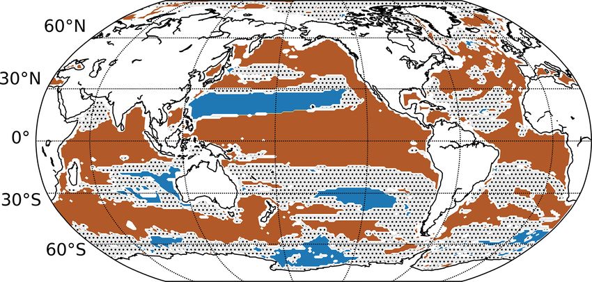
1884 A. Hameau et al.: Is deoxygenation detectable before warming?
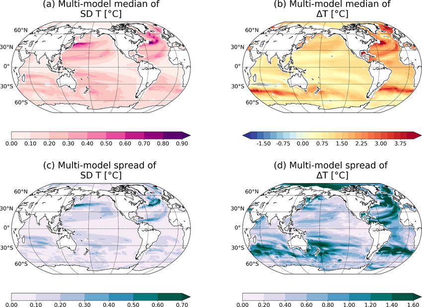
Figure 4. Median (a, b) and spread (c, d) of multi-model natural variability (standard deviation of control simulation; a, c) and changes
by the end of the 21st century (b, d) of ocean temperature between 200 and 600 m. The individual responses for each model are shown in
Figs. S3 and S4.
years 1991 and 2046 for the nine models (see subtitles in (Fig. 1c) and oxygen (Fig. 1f), while spatial patterns are sim-
Fig. 3). The analysis of ToErel (O2 ) for individual models re- ilar for ToErel and ToEabs .
veals some additional notable differences (Fig. 3). GFDL- On a global average, the spread is reduced from ±30 years
ESM2M, GFDL-ESM2G, HadGEM2-CC and CESM1.0 for ToEabs (T ) to ±23 years for ToErel (T ) and from
simulate early emergence in the Southern Ocean, but the ±20 years for ToEabs (O2 ) to ±17 years for ToErel (O2 ). Re-
IPSL models project no emergence of deoxygenation in this gionally, the reduction can be larger. For example, in the
region by the end of the 21st century. In addition, the IPSL equatorial regions, the Atlantic and the Southern Ocean, the
models and the CESM1.0 model show relatively early emer- spread is reduced by 20 to 50 years when computed for
gence in many grid cells of the western tropical Pacific, a ToErel (T ) instead for ToEabs (T ). Similarly, the spread in
region with no emergence in other models. ToErel (O2 ) also ToE(O2 ) is reduced from ±35 to ±5 years in parts the North
diverges across the models in the Atlantic subtropical gyres: Pacific.
in the HadGEM2 and IPSL simulations, oxygen changes
are simulated to emerge relatively early (ToErel (O2 ) ∼ 40 to 3.3 Internal variability and anthropogenic signals
60 years), whereas in the GFDL, MPI and CESM simula-
tions, the changes are not yet detectable by the end of the The ToE allows for a comparison across climate models, by
21st century. combining the amplitude of the climate response to anthro-
pogenic forcing and the amplitude of natural variability in
3.2 Relative versus absolute ToE one metric. The magnitude and the spatial patterns of the
internal variability and of the anthropogenic signal for both
Mapping ToErel for different models is intended to empha- thermocline temperature and oxygen are discussed next.
sise common patterns across models by removing the global The multi-model median of internal variability for ther-
mean bias between models, while model–model differences mocline temperature fluctuates with an amplitude typically
in ToEabs are indicative of an overall model uncertainty. ±0.1 ◦ C in the tropics and the Arctic Ocean, and ±0.5 ◦ C
The multi-model spread for ToEabs is on average larger in mid-to-high latitudes (Fig. 4a). SD(T ) is the largest (up
than the multi-model spread for ToErel for temperature to ±0.9 ◦ C) in the western boundary currents such as the
Biogeosciences, 17, 1877–1895, 2020 www.biogeosciences.net/17/1877/2020/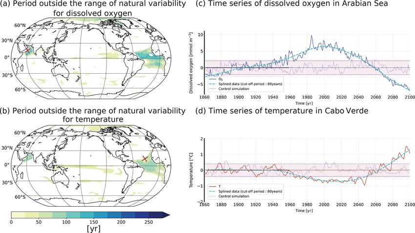
A. Hameau et al.: Is deoxygenation detectable before warming?                                                                       1885

Figure 5. Median (a, b) and spread (c, d) of multi-model natural variability (standard deviation of control simulations; a, c) and changes
by the end of the 21st century (b, d) of O2 between 200 and 600 m. The hatched areas in panel (b) show regions where at least 70 % of the
models do not agree on 1O2 sign. The individual responses for each model are shown in Figs. S5 and S6.

Kuroshio Current and the Gulf Stream. The internally gen-              small (0.1 to 0.3 ◦ C; Fig. 4a). However, early emergence of
erated variability is also relatively large along the equator-         anthropogenic changes can also occur when the signal is rel-
ward flanks of the subtropical gyres. It is also in these regions      atively small, if the variability is even smaller. This is the
where SD(T ) differs most among models (up to ±0.5 ◦ C                 case in the tropical oceans such as in the Arabian Sea, the
along the North Atlantic Current; Fig. 4c).                            equatorial Atlantic and the western equatorial Pacific, where
   In the multi-model median, temperature in the thermocline           water masses warm modestly (up to 1.5 ◦ C) but vary natu-
is projected to increase on global average by 1.2 ± 0.7 ◦ C            rally between 0.1 and 0.2 ◦ C only. It is also the case in the
(Fig. 4b) by the end of the 21st century under the RCP8.5              eastern equatorial Pacific, where the early emergence arises
scenario relative to the period 1861–1959, in accordance with          from the very weak internal variability in the thermocline,
published observational studies (Levitus et al., 2009, 2012;           although the temperature increase (∼ 0.80 ◦ C) is also rela-
Bilbao et al., 2019). Large warming of more than 4.0±0.7 ◦ C           tively weak. In this region, the substantial variability in O2
is projected in the northern North Atlantic and around the             and T is largely confined to the top 200 m. No emergence by
subantarctic water in the Indian and Atlantic oceans (Figs. 4b         the end of the 21st century, such as that simulated in the sub-
and S4). We note that these projections are also characterised         tropical gyres of the Indian and Pacific oceans, results from
with the largest inter-model spread (±1.5 ◦ C; Figs. 4d and            a relatively weak signal combined with a relatively strong
S4), and uncertainties in these regional warming projections           variability in these regions.
are large. Finally, disagreement among models in simulating               Internal variability of dissolved oxygen concentrations is
changes in thermocline temperature is also large in the Arctic         particularly large in the northern North Pacific and North
Ocean, possibly related to different simulated changes in sea          Atlantic, the Southern Ocean and along the equatorward
ice cover (Stroeve et al., 2012; Wang and Overland, 2012).             boundaries of the subtropical gyres with SD(O2 ) of up to
   The combination of a strong signal and small variability            10 mmol m−3 (Fig. 5a). The multi-model spread of SD(O2 )
results in early detection of the changes. This is the case in         (Fig. 5c) is about equally large as the median of SD(O2 )
the Southern Ocean at 45◦ S (in the Atlantic and Indian re-            (Fig. 5a) along the equatorward boundaries of the subtropi-
gions; Fig. 1a), where the anthropogenic warming is strong             cal gyres. Looking at the individual model responses, the O2
(up to 4 ◦ C; Fig. 4b) but the internal variability is relatively      internal variability shows a wide range of different patterns

www.biogeosciences.net/17/1877/2020/                                                            Biogeosciences, 17, 1877–1895, 2020

1886                                                           A. Hameau et al.: Is deoxygenation detectable before warming?

Figure 6. 1ToE defined as ToE(T ) minus ToE(O2 ) for each simulation in the thermocline. Blueish colours indicate earlier emergence of
oxygen. Brownish colours indicate earlier emergence of temperature. The saturated colours mean that one of the variables has not emerged
by 2099. No emergence in both T and O2 is shown by the hatched areas.

                                                                      (Fig. S5). The GFDL and MPI models simulate high inter-
                                                                      nal variability of oxygen in the entire thermocline, whereas
                                                                      CESM, HadGEM2 and IPSL models show high variability
                                                                      regionally.
                                                                         The O2 concentration in the thermocline (Fig. 5b) is pro-
                                                                      jected to decrease under global warming, in accordance with
                                                                      previous model studies (e.g. Sarmiento et al., 1998; Cocco
                                                                      et al., 2013; Bopp et al., 2017). The anthropogenic decrease
                                                                      in O2 is large in the Southern Ocean, in the North Pacific
                                                                      subtropical gyre and in the North Atlantic subpolar gyre. In
Figure 7. Summary map showing the regions where oxygen
                                                                      tropical regions, the changes are projected to be small, except
changes emerge before temperature changes (blue areas; 1ToE > 0       for the western Indian Ocean, where more than 70 % of the
with 1ToE = ToE(T ) − ToE(O2 )) and where temperature changes         models project an increase of O2 concentration. The simu-
emerge before oxygen changes (brown areas; 1ToE < 0) for at least     lated O2 changes differ most across models in high latitudes
seven out of nine models. The dashed areas show the regions where     and in the subpolar gyres, as well as in the equatorial Indian
more than three models differ in the sign of 1ToE.                    Ocean (Fig. 5d).
                                                                         Despite differences in the simulated magnitude of O2
                                                                      changes and internal variability patterns of O2 between the
                                                                      different models, the resulting ToErel (O2 ) are robust across

Biogeosciences, 17, 1877–1895, 2020                                                         www.biogeosciences.net/17/1877/2020/
A. Hameau et al.: Is deoxygenation detectable before warming? 1887
Figure 8. Anthropogenic changes (2070–2099 CE minus 1861–1959 CE) in [-AOU] in the thermocline for each model.
models. For example, the decrease in O2 spans from −12 3.4 Comparison of ToE(O2 ) with ToE(T )
to −40 mmol m−3 (Fig. S6) and SD(O2 ) spans from ±5 to
±15 mmol m−3 (Fig. S5) in the central North Pacific. More-
In general, temperature changes are detectable before O2
over, the spatial locations of the maximum O2 depletion dif-
changes in around 64 ± 11 % of the thermocline (yellow to
fer across the models. However, ToErel (O2 ) in this region
brown colours in Fig. 6). As discussed in Sect. 3.1, the an-
is within ∼ 10 years (Fig. 1d), with a relatively low spread
thropogenic O2 signal emerges late or not at all in many
(±10 years) compared to ToEabs (O2 ) (±30 years). Another
low-latitude regions, while the anthropogenic warming sig-
example is the CESM model. The very early detection of
nal is emerging in most regions and typically early around
anthropogenic changes (for temperature and oxygen) in the
the Equator. However, there are also areas where anthro-
CESM model described in Sect. 3.1, results from a partic-
pogenic deoxygenation is detectable earlier than anthro-
ularly weak internal variability (Figs. S3i and S5i; see also
pogenic warming in all models (green to blue colours in
Hameau et al., 2019) combined with a high climate sensitiv-
Fig. 6). These cover 35 ± 11 % of the global thermocline
ity of the model (Figs. S4i and S6i). The ToErel allows the
in the nine models. They are mainly located in the mid-
comparison of ToE resulting from CESM output with the re-
latitudes, especially between ∼ 15 and 30◦ N in the North
sults from the eight models in spite of these model–model
Pacific, around Antarctica (including the Ross and Weddell
differences (Figs. 2 and 3).
seas), along the Western Australian Current and the Pacific
southern subtropical gyre region. Model results for the At-
lantic subtropical gyres are mixed. Some models suggest O2
changes to be detectable earlier than T changes (HadGEM2
and the IPSL family), whereas in other models the O2 signal
does not even emerge.
www.biogeosciences.net/17/1877/2020/ Biogeosciences, 17, 1877–1895, 20201888 A. Hameau et al.: Is deoxygenation detectable before warming?
tration of the anthropogenic warming signal from the surface
to the interior and similarly the penetration of the thermally
driven O2 signal ([O2,sol ]). The detection of the temperature
changes is thus delayed compared to AOU and O2 . There
are some exceptions to this relationship between [-AOU] and
the earlier emergence of O2 than T . For example, O2 change
emerges before warming in the GFDL model around 30◦ S
and 120◦ W, although [-AOU] is increasing in this region.
However, warming is emerging very late as the GFDL mod-
els simulate weak warming and even some cooling (Fig. S4)
in this part of the thermocline. Thus, in this special case, the
early emergence of O2 relative to T is due to the absence of
large warming in a region with notable temperature internal
variability.
Regions where the warming signal is detectable before the
deoxygenation are typically associated with an increase in
Figure 9. Density distribution of [-AOU] changes by 2099 for the [-AOU]. Such increase counteracts the decrease in [O2,sol ],
grid points where the O2 signal emerges first (blue) and where
leading to relatively smaller changes in [O2 ], which are thus
the temperature signal emerges first (brown) in the thermocline
for the ensemble of nine models. Each distribution is centred
often not detectable. There are again a few exceptions. For
around the median (dashed blue: −10.8 mmol m−3 ; dashed brown: example, the IPSL models simulate a decrease in [-AOU] in
3.3 mmol m−3 ). the northern North Pacific but an earlier ToE for T than for
O2 in this region.
In summary, anthropogenic change in temperature is de-
tectable earlier than anthropogenic change in O2 in most of
The exact locations of relatively early emergence of O2 the global ocean. However, there are large ocean regions
differ across models. Hence, the regions where at least seven where anthropogenic O2 changes are detectable earlier in
out of the nine models show consistently an earlier emer- the thermocline in all models. Early emergence of deoxy-
gence of O2 than T is smaller and amounts to 17 % of the genation relative to warming is typically detected in regions
global thermocline area. As shown in Fig. 7 (blue areas), the where thermocline ventilation and [-AOU] are decreasing
O2 signal emerges consistently in at least seven models be- over the simulation and late emergence of O2 changes where
fore the T signal in parts of the Pacific subtropical gyres, the ventilation and [-AOU] are increasing.
Southern Ocean and the southeast Indian Ocean.
A mechanistic explanation of early or late emergence of
the O2 signal relative to the temperature signal is not straight- 4 Discussion and conclusions
forward as two ratios (S/N ) are involved. Nevertheless,
changes in apparent oxygen utilisation (1[-AOU]; Fig. 8) We analysed the time of emergence (ToE) of human-induced
provide some insight into underlying mechanisms. We use changes in oxygen (O2 ) concentrations and temperature (T )
1[-AOU] as a proxy for changes in water mass age and ven- in the thermocline (200–600 m) using nine Earth system
tilation, as noted in Sect. 2.2. model simulations of the climate over the historical and the
Regions with early emergence of anthropogenic O2 com- future period. Using ToE as a metric allows for the assess-
pared to T show typically a decrease in [-AOU] (Fig. 6 ver- ment of anthropogenic changes by comparing the magnitude
sus Fig. 8), whereas regions with early emergence of T com- of the human-induced changes with the magnitude of internal
pared to O2 show typically an increase in [-AOU]. For ex- variability. Both the magnitude of anthropogenic change and
ample, [-AOU] is decreasing in 77 ± 8 % of the areas with internal variability are model dependent, rendering the abso-
early emergence of O2 , while only 22 ± 8 % of these regions lute year of ToE strongly model dependent. Evaluating differ-
show an increase in [-AOU] (Fig. 9; blue). In most regions ences in absolute year of ToE, however, can obscure impor-
where T is emerging before O2 (Fig. 9; brown), [-AOU] tant model agreement upon the spatial patterns and progres-
is increasing (62 ± 12 %). A decreasing trend in [-AOU] is sion of emergence within a multi-variable framework. We
indicative of a reduced ventilation induced by upper ocean therefore introduce a new metric, the relative ToE (ToErel ),
warming and increased stratification (e.g. Capotondi et al., to better compare ToE across different models and variables.
2012). A more sluggish ventilation slows the supply of O2 ToErel is computed by subtracting the global mean ToE from
from the surface to the ocean interior. Consequently, thermo- the ToE field. Absolute years of emergence are thus not con-
cline [O2 ] and [-AOU] are both decreasing. This leads to a sidered by this metric and it only illustrates whether a signal
strong and thus early detectable anthropogenic deoxygena- emerges relatively early or late for a given model. We inves-
tion. In addition, a more sluggish ventilation slows the pene- tigated whether anthropogenic T or O2 changes emerge first
Biogeosciences, 17, 1877–1895, 2020 www.biogeosciences.net/17/1877/2020/A. Hameau et al.: Is deoxygenation detectable before warming? 1889 and link patterns of ToE(T )–ToE(O2 ) to changes in apparent to estimate the signal. They showed that ideally the noise (N) oxygen utilisation (1[-AOU]) and ventilation of the thermo- component of ToE should be estimated from simulations that cline. In addition, we also identified the processes for ear- include natural variability forced by explosive volcanic erup- lier/later detection in O2 changes compared to temperature tions and changes in total solar irradiance, especially when changes. assessing regional- to global-scale ToE estimates. However, This multi-model study relies only on results from only these authors also find that on a grid cell scale, internal vari- four different model families (GFDL-ESM, HadGEM2-CC, ability is typically the dominant contribution to overall natu- IPSL, MPI-ESM and CESM), applied in nine model configu- ral variability during the last millennium. Therefore, estimat- rations. All model configurations available from CMIP5 that ing the noise from control simulations that include internal provide three-dimensional fields for O2 and T for the con- variability only, as done in this study, appears justified. trol, historical and future RCP8.5 scenario simulations have Another limitation of our study lies in the assumption that been incorporated into the analysis. Nevertheless, using a the anthropogenic signal emerges from interannual to multi- larger model ensemble would increase confidence in our re- decadal internal variability. The anthropogenic signal S and sults (Knutti and Sedláček, 2013). the noise N are estimated by smoothing the model output A limitation of our study is that all the Earth system mod- with a multi-decadal spline filter. Any potential natural cen- els included have a relatively coarse resolution for simulat- tennial variations are retained in the signal S and removed ing the complex processes in the O2 minimum zones (Mar- from the noise N. Results from a forced simulation over the golskee et al., 2019). Earth system models diverge in pro- past millennium with CESM1.0 show that potential biases in jecting physical and biogeochemical changes in these regions ToE arising from the neglect of long-term natural variability (Brandt et al., 2015; Cabré et al., 2015). Some models used in are small for this model (Hameau et al., 2019). However, our this study project a large increase in [-AOU] (Fig. 8) and con- multi-model analysis reveals centennial variations in some siderable warming (Fig. S6) in the eastern tropical Atlantic, grid cells and models causing multiple emergence of the sig- likely indicative of a reduced upwelling (Gnanadesikan et al., nal from the noise (Fig. A2). This may bias the detection of 2007). Observations show a decrease in O2 and an expan- the anthropogenic signal towards early emergence. Here, we sion of hypoxia in the tropics (Stramma et al., 2008, 2012) constrained detection to partly circumvent problems with re- over recent decades, contradicting the long-term projections emerging signals; we require that the trend of the signal at the from some models. However, these observed trends in the time of emergence must have the same sign as the change be- tropics may also be a result of natural variability acting on tween the last and first 30 model years. Re-emerging signals multi-decadal timescales associated with the Pacific Decadal are found in only a few grid cells, except in HadGEM2, and Oscillation. centennial natural variability appears to play a minor role in Comparing ToE estimates from different studies is del- these simulations. We expect therefore that our estimates of icate due to the model and method dependencies of ToE. ToE are reliable for the model ensemble. Although the generic definition of ToE is under consensus, Published studies addressing the detection of anthro- the methodologies applied to estimate ToE differ in the pub- pogenic ocean warming focus on temperature at sea sur- lished literature, as mentioned in the introduction (e.g. IPCC, face. To our knowledge, only a single study (Hameau et al., 2019). Depending on the spatial and temporal scale of a given 2019) using output from a single model is assessing ToE(T ) variable, the threshold for which emergence is defined and in the thermocline. Yet, the thermocline is a habitat for the reference period applied, the absolute value of ToE can many fish and other species. Warming in combination with differ. In addition, the ToE also depends on the definition other stressors, such as deoxygenation, ocean acidification of the background variability, here acting as noise (Hameau and hypocapnia, may reduce the habitat suitability of marine et al., 2019). Estimating the background noise as the stan- ecosystems in a future climate (e.g. Deutsch et al., 2015; Gat- dard deviation (SD) of the internal chaotic variability from tuso et al., 2015; Breitburg et al., 2018; Cheung et al., 2018). the control simulation (Frölicher et al., 2016) or as the SD of Multi-tracer analyses contribute to a better understanding of the variability from the industrial period (after removing an- the potential impact on marine ecosystems in a changing thropogenic trends; Keller et al., 2015; Henson et al., 2016) ocean. results in earlier ToE for both O2 and T as when estimat- We find that thermocline anthropogenic warming emerges ing the noise from the total (internal and externally forced) first in low latitudes, followed by the Southern Ocean and the natural variability over the last millennium. Yet, the finding high northern latitudes. No emergence is detected in parts that anthropogenic O2 change emerges before anthropogenic of the subtropical gyres of the Pacific and Indian oceans. warming in large ocean regions is robust across investigated The rapid emergence at low latitudes is explained by the choices. The anthropogenic signal is frequently computed as small internal variability but moderate to strong warming sig- a linear trend over a few decades (Rodgers et al., 2015; Hen- nals. Exceptions are the subtropical gyres in the Atlantic, son et al., 2017; Tjiputra et al., 2018). However, the resulting where it takes approximately two additional decades to de- slope depends on the time window used to calculate the lin- tect the temperature changes, mainly because of the relatively ear trend. Hameau et al. (2019) use a low-pass-filtered output large internal variability there. The warming in mid- to high- www.biogeosciences.net/17/1877/2020/ Biogeosciences, 17, 1877–1895, 2020
1890                                                         A. Hameau et al.: Is deoxygenation detectable before warming?

latitude thermocline emerges approximately 60 to 80 years          the nine models, an area covering 35 ± 11 % of the global
later than in low latitudes. No emergence is simulated for         thermocline shows emergence in O2 change before tempera-
the Pacific and Indian subtropical gyres, because the changes      ture change. Yet, the exact locations of these patterns differ
in temperature are relatively small and the internal variabil-     across models. Only 17 % of the global thermocline show
ity relatively high there (in accordance with Hameau et al.,       agreement (seven out of the nine models) on earlier emer-
2019). For comparison, surface temperature changes emerge          gence of O2 changes prior to T changes; thus, our multi-
at first in low latitudes and then in midlatitudes (Henson         model analysis confirms earlier findings using output from
et al., 2017).                                                     a single model only (Hameau et al., 2019). The early emer-
   The time of emergence spatial pattern of thermocline            gence of O2 suggests that the monitoring of biogeochem-
oxygen changes is almost opposite to the one of tempera-           ical variables would be particularly useful to detect early
ture. Rapid emergence for O2 is simulated at midlatitudes,         signals of anthropogenic change in the ocean interior (Joos
whereas low latitudes generally do not experience emergence        et al., 2003). Multi-tracer observations of both physical and
of the O2 signal by the end of the 21st century (Rodgers et al.,   biogeochemical variables may enable an earlier detection of
2015; Frölicher et al., 2016; Long et al., 2016).                  potential changes than temperature-only data (Keller et al.,
   Although internal variability is low in the tropical regions,   2015) in specific regions and for specific processes.
the O2 signal does not emerge by 2100. This is because the            Hameau et al. (2019) established a direct link between the
projected changes are also small. This is due to the opposite      early emergence in O2 with a slowdown of ventilation. A
responses of O2 components. The thermal component is sim-          weaker ventilation leads to a decrease in [-AOU], and there-
ulated to decrease (due to temperature increase), but [-AOU]       fore a reduction in O2 , with a minor role for organic mat-
is on average projected to increase, counteracting the O2,sol      ter export changes in their simulation. We used [-AOU] as a
trend (Frölicher et al., 2009; Cocco et al., 2013; Bopp et al.,    ventilation age proxy for our model ensemble and concluded
2017). Some regions show similar relative ToE but for dif-         that the slowdown of the ventilation induces O2 changes to be
ferent reasons. For example, in the North Pacific subtropical      detectable before T changes in many regions. A slower ven-
gyre and the Southern Ocean, both the oxygen depletion and         tilation seems to shift the balance between O2 supply from
the internal variability are relatively strong. In the Arabian     the surface and O2 consumption by organic matter reminer-
Sea, internal variability and anthropogenic response are both      alisation. Moreover, a more stratified upper ocean delays the
rather weak. Nevertheless, the S/N ratio results in very sim-      propagation of the temperature signal from the surface into
ilar relative ToE for all these regions.                           the subsurface waters. Note that the exact locations of early
   The transient climate response of the individual models         O2 emergence and reductions in [-AOU] and ventilation di-
and therefore the ocean heat uptake, thermocline warming           verge among the models. This is partly due to model biases in
and deoxygenation can substantially differ among models            terms of ocean dynamics. In addition, the use of depth coor-
(Bopp et al., 2013). The simulated internal variability also       dinates to define a thermocline layer from 200 to 600 m may
differs considerably across models (e.g. Resplandy et al.,         lead in our analysis to the inclusion of different water masses
2015; Frölicher et al., 2016). ToE values computed from            for different models. Another approach would be to perform
CESM1.0 projections, for example, differ by many decades           the analysis on isopycnal levels instead on depth levels.
in absolute values from other CMIP5 models, mostly due to             To conclude, normalising ToE across models (relative
a very weak internal variability. Nijsse et al. (2019) suggest     ToE) or estimating ToE in relation to another variable
that the magnitude of simulated decadal variability and cli-       (ToE(T ) – ToE(O2 )) reduces the multi-model spread aris-
mate sensitivity might be correlated. They suggest that mod-       ing from method and model dependencies. We find that in
els with a high climate sensitivity tend to simulate a high        about 35 % of the thermocline anthropogenic O2 depletion
decadal variability. This may imply a compensation between         emerges before anthropogenic warming. This relative early
the simulated signal and noise on the decadal scale. To ex-        emergence of O2 is linked to a more sluggish ventilation of
tract valuable insights as to the relative spatial and temporal    these subsurface waters under global warming. Our study
features of emergence across models and variables, we intro-       also suggests that temperatures in the thermocline have al-
duced a new metric, the relative time of emergence. Normal-        ready left the bounds of internal variability in much of the
ising the ToE using the globally averaged ToE as reference         tropical ocean and that temperatures will have left these
allows for a more direct comparison with the other models.         bounds in most of the thermocline by 2100 under unabated
As a result, the patterns and time of emergence of anthro-         global warming.
pogenic changes in O2 and warming in CESM1.0 are more
coherent with the other models for ToErel than for the abso-
lute ToE.
   Following Hameau et al. (2019), we compared the ToE(T )
with the ToE(O2 ) in nine models. We find that the anthro-
pogenic decline in O2 emerges before anthropogenic warm-
ing in a significant part of the thermocline. On average across

Biogeosciences, 17, 1877–1895, 2020                                                    www.biogeosciences.net/17/1877/2020/
A. Hameau et al.: Is deoxygenation detectable before warming?                                                                         1891

Appendix A

Figure A1. Illustration of the ToE method by using simulated oxygen concentration of the MPI-ESM-LR model averaged over 200–600 m in
one grid cell in the western North Pacific. The dark blue line shows that temporal evolution of oxygen anomalies from 1860 to 2099 relative
to preindustrial concentrations (1860–1959). The two pink lines indicate the magnitude of the noise, N , which is computed as 2 standard
deviations from annual output of the control simulation. The anthropogenic signal, S, is the simulated oxygen concentration over 1860 to
2099 from the forced simulation splined with a 80-year cut-off period (dashed cyan). Here, the resulting ToE is the intersection between the
lower limit of the noise and the splined signal (vertical dashed line).

Figure A2. Period outside the range of natural variability for (a) oxygen concentration and (b) temperature in the thermocline for the model
HadGEM2. The time series show two examples of the temporal evolution of the oxygen concentration (c) and temperature (d) for a single
grid point: red crosses in panels (a, b): Arabian Sea (c) and equatorial Atlantic (d).

www.biogeosciences.net/17/1877/2020/                                                             Biogeosciences, 17, 1877–1895, 2020
1892                                                              A. Hameau et al.: Is deoxygenation detectable before warming?

Data availability. The CMIP5 simulations are available on https://      References
esgf-node.ipsl.upmc.fr (last access: June 2019, Taylor et al., 2012).
Results from the CESM1.0 simulations are available upon request.
                                                                        Aumont, O. and Bopp, L.: Globalizing results from ocean in situ
                                                                           iron fertilization studies, Global Biogeochem. Cy., 20, GB2017,
Supplement. The supplement related to this article is available on-        https://doi.org/10.1029/2005GB002591, 2006.
line at: https://doi.org/10.5194/bg-17-1877-2020-supplement.            Battaglia, G. and Joos, F.: Hazards of decreasing marine oxy-
                                                                           gen: the near-term and millennial-scale benefits of meeting
                                                                           the Paris climate targets, Earth Syst. Dynam., 9, 797–816,
                                                                           https://doi.org/10.5194/esd-9-797-2018, 2018.
Author contributions. All authors contributed to the discussion and
                                                                        Bilbao, R. A. F., Gregory, J. M., Bouttes, N., Palmer, M. D.,
the writing of the paper.
                                                                           and Stott, P.: Attribution of ocean temperature change to an-
                                                                           thropogenic and natural forcings using the temporal, verti-
                                                                           cal and geographical structure, Clim. Dynam., 53, 5389–5413,
Competing interests. The authors declare that they have no conflict        https://doi.org/10.1007/s00382-019-04910-1, 2019.
of interest.                                                            Bopp, L., Le Quéré, C., Heimann, M., Manning, A. C., and Mon-
                                                                           fray, P.: Climate-induced oceanic oxygen fluxes: Implications
                                                                           for the contemporary carbon budget, Global Biogeochem. Cy.,
Special issue statement. This article is part of the special issue         16,https://doi.org/10.1029/2001GB001445, 2002.
“Ocean deoxygenation: drivers and consequences – past, present          Bopp, L., Resplandy, L., Orr, J. C., Doney, S. C., Dunne, J. P.,
and future (BG/CP/OS inter-journal SI)”. It is a result of the Inter-      Gehlen, M., Halloran, P., Heinze, C., Ilyina, T., Séférian, R.,
national Conference on Ocean Deoxygenation, Kiel, Germany, 3–7             Tjiputra, J., and Vichi, M.: Multiple stressors of ocean ecosys-
September 2018.                                                            tems in the 21st century: projections with CMIP5 models,
                                                                           Biogeosciences, 10, 6225–6245, https://doi.org/10.5194/bg-10-
                                                                           6225-2013, 2013.
Acknowledgements. Angélique Hameau, Fortunat Joos and                   Bopp, L., Resplandy, L., Untersee, A., Mezo, P. L., and
Thomas L. Frölicher thank Christoph Raible and Flavio Lehner               Kageyama, M.: Ocean (de)oxygenation from the Last Glacial
for providing CESM output. We also thank the World Climate                 Maximum to the twenty-first century: insights from Earth
Research Programme’s Working Group on Coupled Modelling,                   System models, Philos. T. Roy. Soc. A, 375, 20160323,
which is responsible for CMIP5, and the climate modelling groups           https://doi.org/10.1098/rsta.2016.0323, 2017.
for producing and making available their model output. We thank         Brandt, P., Bange, H. W., Banyte, D., Dengler, M., Didwischus,
the anonymous referee, Sarah Schlunegger and Ming Li for their             S.-H., Fischer, T., Greatbatch, R. J., Hahn, J., Kanzow, T.,
time and effort.                                                           Karstensen, J., Körtzinger, A., Krahmann, G., Schmidtko, S.,
                                                                           Stramma, L., Tanhua, T., and Visbeck, M.: On the role of circula-
                                                                           tion and mixing in the ventilation of oxygen minimum zones with
Financial support. This research has been supported by the                 a focus on the eastern tropical North Atlantic, Biogeosciences,
Oeschger Center for Climate Change Research, the Swiss National            12, 489–512, https://doi.org/10.5194/bg-12-489-2015, 2015.
Science Foundation (nos. 200020_172476 and PP00P2_170687)               Breitburg, D., Levin, L. A., Oschlies, A., Grégoire, M., Chavez,
and the CSCS Swiss National Supercomputing Center, providing               F. P., Conley, D. J., Garçon, V., Gilbert, D., Gutiérrez, D., Isensee,
computing resources. This publication has received funding from            K., Jacinto, G. S., Limburg, K. E., Montes, I., Naqvi, S. W. A.,
the European Union’s Horizon 2020 research and innovation pro-             Pitcher, G. C., Rabalais, N. N., Roman, M. R., Rose, K. A.,
gramme under grant agreement no. 820989 (project COMFORT,                  Seibel, B. A., Telszewski, M., Yasuhara, M., and Zhang, J.: De-
Our common future ocean in the Earth system – quantifying cou-             clining oxygen in the global ocean and coastal waters, Science,
pled cycles of carbon, oxygen, and nutrients for determining and           359, 6371, https://doi.org/10.1126/science.aam7240, 2018.
achieving safe operating spaces 30 with respect to tipping points).     Cabré, A., Marinov, I., Bernardello, R., and Bianchi, D.: Oxy-
The work reflects only the authors’ view; the European Commis-             gen minimum zones in the tropical Pacific across CMIP5 mod-
sion and their executive agency are not responsible for any use that       els: mean state differences and climate change trends, Biogeo-
may be made of the information the work contains.                          sciences, 12, 5429–5454, https://doi.org/10.5194/bg-12-5429-
                                                                           2015, 2015.
                                                                        Capotondi, A., Alexander, M. A., Bond, N. A., Curchitser, E. N.,
Review statement. This paper was edited by Kenneth Rose and re-            and Scott, J. D.: Enhanced upper ocean stratification with cli-
viewed by Sarah Schlunegger, Ming Li, and one anonymous referee.           mate change in the CMIP3 models, J. Geophys. Res.-Oceans,
                                                                           117, C04031, https://doi.org/10.1029/2011JC007409, 2012.
                                                                        Chen, X. and Tung, K.-K.: Global surface warming enhanced by
                                                                           weak Atlantic overturning circulation, Nature, 559, 387–391,
                                                                           https://doi.org/10.1038/s41586-018-0320-y, 2018.
                                                                        Cheng, L., Trenberth, K. E., Fasullo, J., Boyer, T., Abraham, J.,
                                                                           and Zhu, J.: Improved estimates of ocean heat content from 1960
                                                                           to 2015, Sci. Adv., 3, 3, https://doi.org/10.1126/sciadv.1601545,
                                                                           2017.

Biogeosciences, 17, 1877–1895, 2020                                                             www.biogeosciences.net/17/1877/2020/
You can also read