Sea ice volume variability and water temperature in the Greenland Sea
←
→
Page content transcription
If your browser does not render page correctly, please read the page content below
The Cryosphere, 14, 477–495, 2020
https://doi.org/10.5194/tc-14-477-2020
© Author(s) 2020. This work is distributed under
the Creative Commons Attribution 4.0 License.

Sea ice volume variability and water temperature
in the Greenland Sea
Valeria Selyuzhenok1,2 , Igor Bashmachnikov1,2 , Robert Ricker3 , Anna Vesman1,2,4 , and Leonid Bobylev1
1 Nansen International Environmental and Remote Sensing Centre, 14 Line V.O. 7, 199034 St. Petersburg, Russia
2 Department  of Oceanography, St. Petersburg State University, 10 Line V.O. 33, 199034 St. Petersburg, Russia
3 Alfred-Wegener-Institut, Helmholtz-Zentrum für Polar- und Meeresforschung,

Klumannstr. 3d, 27570 Bremerhaven, Germany
4 Atmosphere-sea ice-ocean interaction department, Arctic and Antarctic Research Institute,

Bering Str. 38, 199397 St. Petersburg, Russia

Correspondence: Valeria Selyuzhenok (valeria.selyuzhenok@niersc.spb.ru)

Received: 22 May 2019 – Discussion started: 26 June 2019
Revised: 21 November 2019 – Accepted: 4 December 2019 – Published: 5 February 2020

Abstract. This study explores a link between the long-term       1   Introduction
variations in the integral sea ice volume (SIV) in the Green-
land Sea and oceanic processes. Using the Pan-Arctic Ice         The Greenland Sea is a key region of deep ocean convec-
Ocean Modeling and Assimilation System (PIOMAS, 1979–            tion (Marshall and Schott, 1999; Brakstad et al., 2019) and
2016), we show that the increasing sea ice volume flux           an inherent part of the Atlantic Meridional Overturning Cir-
through Fram Strait goes in parallel with a decrease in SIV in   culation (AMOC) (Rhein et al., 2015; Buckley and Marshall,
the Greenland Sea. The overall SIV loss in the Greenland Sea     2016). The intensity of convection is governed by buoyancy
is 113 km3 per decade, while the total SIV import through        (heat and freshwater) fluxes at the ocean–atmosphere bound-
Fram Strait increases by 115 km3 per decade. An analysis         ary, as well as oceanic buoyancy advection into the region.
of the ocean temperature and the mixed-layer depth (MLD)         The freshwater is thought to play the principal role in long-
over the climatic mean area of the winter marginal sea ice       term buoyancy balance of the upper Greenland Sea (Meincke
zone (MIZ) revealed a doubling of the amount of the upper-       et al., 1992; G. Alekseev et al., 2001). The positive local
ocean heat content available for the sea ice melt from 1993      precipitation–evaporation exchange accounts for only 15 %
to 2016. This increase alone can explain the SIV loss in the     of the freshwater balance in the Nordic Seas. Approximately
Greenland Sea over the 24-year study period, even when ac-       half of the fresh water anomaly in the Nordic Seas originates
counting for the increasing SIV flux from the Arctic. The        from the freshwater flux through Fram Strait, which forms
increase in the oceanic heat content is found to be linked to    by freshening of the upper ocean due to sea ice melt in the
an increase in temperature of the Atlantic Water along the       Arctic Ocean and by solid sea ice transport melting outside
main currents of the Nordic Seas, following an increase in       the Arctic Ocean (Serreze et al., 2006; Peterson et al., 2006;
the oceanic heat flux from the subtropical North Atlantic. We    Glessmer et al., 2014).
argue that the predominantly positive winter North Atlantic         The general surface circulation in the region is shown in
Oscillation (NAO) index during the 4 most recent decades,        Fig. 1a. The upper 500 m in the western Greenland Sea is
together with an intensification of the deep convection in the   formed by mixing the Polar Water (PW), with a tempera-
Greenland Sea, is responsible for the intensification of the     ture close to freezing and salinity from 33 to 34, and the At-
cyclonic circulation pattern in the Nordic Seas, which results   lantic Water (AW), with a temperature over 3 ◦ C and salinity
in the observed long-term variations in the SIV.                 around 34.9, recirculating in the southern part of the Fram
                                                                 Strait (Moretskij and Popov, 1989; Langehaug and Falck,
                                                                 2012; Jeansson et al., 2017). The maximum PW content is
                                                                 found in the upper 200 m of the Greenland shelf and quickly

Published by Copernicus Publications on behalf of the European Geosciences Union.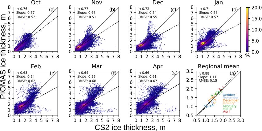
478                                                                  V. Selyuzhenok et al.: Sea ice and ocean water temperature

decreases in the off-shelf direction (Håvik et al., 2017). The         sea ice tongue was occasionally formed, a sea ice pattern ex-
AW is found below the PW. Its core is observed in the sea-             tended eastwards from the east Greenland shelf northwest of
ward branch of the East Greenland Current (EGC), trapped               Jan Mayen (Wadhams et al., 1996; Comiso et al., 2001). The
by the continental slope. The central part of the Greenland            regression of the first empirical orthogonal function (EOF) of
Sea represents a mixture of the AW and the PW with the                 the sea ice extent to sea level pressure shows a weak inverse
Greenland Sea Intermediate Water (with a temperature of                relation with the NAO-like pattern with a correlation coeffi-
−0.4 to −0.8 ◦ C and salinity of ∼ 34.9). The core of the              cient of −0.4. During the negative NAO phase, a reduction
Greenland Sea Intermediate Water is found at 500–1000 m.               of the northerly wind permits a more intensive westward Ek-
The Greenland Sea Deep Water (with a temperature of −0.8               man drift of sea ice into the Greenland Sea interior, which fa-
to −1.2 ◦ C and salinity ∼ 34.9) is found below 1000 m. The            vors formation of the large Odden tongue (Shuchman et al.,
latter two water masses are formed by advection of interme-            1998; Germe et al., 2011). The Odden tongue area shows a
diate and deep water coming from the Arctic Eurasian basin             strong negative correlation with the air temperature (−0.7)
through Fram Strait, mixed with the recirculating Atlantic             over Jan Mayen and with the local sea surface temperature
Water by winter convection (Moretskij and Popov, 1989;                 (−0.9) (Comiso et al., 2001). Having stronger correlations
Alekseev et al., 1989; Langehaug and Falck, 2012). The con-            with water temperature, the negative correlation of the sea
vection depth in the Greenland Sea often exceeds 1500 m                ice area with the air temperature might be an artifact, as both
(Wadhams et al., 2004; Latarius and Quadfasel, 2016; Bash-             are oppositely affected by the oceanic heat release to the at-
machnikov et al., 2019).                                               mosphere (Germe et al., 2011).
   The sea ice conditions in the Greenland Sea are defined                 The ocean clearly plays an important role in the sea ice for-
by sea ice import through Fram Strait and by local ice for-            mation and melt in the region. In particular, it is speculated
mation and melt. The Fram Strait sea ice area (Vinje and               that the oceanic convection in the region favors a more inten-
Finnekåsa, 1986; Kwok et al., 2004) and volume flux (Kwok              sive warm water flux from the south, affecting the air tem-
et al., 2004; Ricker et al., 2018) are primarily controlled by         perature and the sea ice extent (Visbeck et al., 1995). How-
variations in the sea ice drift, which, in turn, are driven by the     ever, presently there is a lack of investigation linking oceanic
large atmospheric circulation patterns. Most of the variabil-          processes with the sea ice variability in the Greenland Sea
ity of the atmospheric circulation and drift patterns is cap-          (Comiso et al., 2001; Kern et al., 2010).
tured by the phase of the Arctic Oscillation (AO) or of its                Both sea ice area flux through Fram Strait and local sea
regional counterpart – the North Atlantic Oscillation (NAO)            ice processes in the Greenland Sea show changes over re-
(Marshall et al., 2001). The positive AO (or NAO) phase in-            cent decades. An overall reduction in sea ice extent has
tensifies northerly winds that drive more intensive ice trans-         been observed in the region since 1979 (Moore et al., 2015;
port through Fram Strait (Kwok et al., 2004). There is a mod-          Onarheim et al., 2018). In particular, a reduction in winter
erate correlation (0.62) between the NAO index (excluding              sea ice area is observed in the region of Odden ice tongue
extreme negative NAO events) and winter sea ice area flux              formation since the 2000s (Rogers and Hung, 2008; Kern
through Fram Strait over 24 years of satellite observations            et al., 2010; Germe et al., 2011). Concurrently, an increase
(1978–2002) (Kwok et al., 2004). A higher correlation (0.70)           in the sea ice area flux through Fram Strait since 1979 was
between NAO index and winter sea ice volume flux (2010–                reported by Kwok et al. (2004) and Smedsrud et al. (2017).
2017) is reported by Ricker et al. (2018). It is also argued           A combined time series of sea ice volume flux through Fram
that the interannual variations in the sea ice area flux through       Strait (1990–1996 Vinje et al., 1998; 1991–1999 Kwok et al.,
Fram Strait even more strongly linked to the Arctic Dipole             2004; and 2003–2008 Spreen et al., 2009) shows a shift to-
pattern, since it explains a higher fraction of the observed in-       wards lower fluxes in the early 2000s compared to the 1990s
terannual variations in the sea ice area flux than either the          (Spreen et al., 2009). However, the later study of Ricker et al.
AO or the NAO (Wu et al., 2006). The Arctic Dipole pat-                (2018) revealed that the sea ice volume flux in 2010–2017 is
tern is derived as the second sea level pressure EOF over the          similar to that in the 1990s. Due to different uncertainties in
Arctic, which has two centers of action: over the Laptev and           the data and different methodologies used in those studies,
Kara seas and over the Canadian Archipelago. The pattern               it is not possible to merge the results to get an uninterrupted
represents an important mechanism regulating the ice export            dataset for the entire period from 1990 to 2017. Although
through Fram Strait (Wu et al., 2006).                                 individual studies do not reveal significant trends in the sea
   The sea ice production in the Greenland Sea takes place             ice volume flux through Fram Strait, the overall tendency re-
east of the shelf between 71 and 75◦ N and north of 75◦ N              mains unknown.
within the highly dynamic pack ice transported southwards                  In this paper we further explore a link between sea ice vol-
along the Greenland coast. The latter fills in cracks and leads        ume variability in the Greenland Sea and oceanic processes.
and can reach considerable thickness. The sea ice forming              The first objective is to estimate the sea ice mass balance in
east of the shelf is mainly thin newly formed ice. The highest         the Greenland Sea from local sea ice formation or melt and
interannual variations in sea ice area is observed between 71          from sea ice advection in or out of the sea, respectively. We
and 75◦ N (Germe et al., 2011). In the region that the Odden           extend this analysis back to 1979 using the Pan-Arctic Ice

The Cryosphere, 14, 477–495, 2020                                                            www.the-cryosphere.net/14/477/2020/
V. Selyuzhenok et al.: Sea ice and ocean water temperature 479
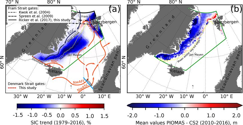
Figure 1. The study region is marked with the green box. (a) Linear trends in the mean October–April NSIDC sea ice concentration (SIC)
over the period 1979–2016 (Comiso, 2015). The black lines show gates used for estimation of the sea ice volume flux through Fram Strait.
Mean winter sea ice edge is shown with the dashed yellow line, and the shelf break (500 m isobath) is shown with the dashed gray line. EGC
is the East Greenland Current, NIIC is the North Icelandic Irminger Current, NwAFC is the Norwegian Atlantic Front Current, NwASC is
the Norwegian Atlantic Slope Current and WSC is the West Spitsbergen Current. (b) Mean difference between mean PIOMAS and CS2
effective sea ice thickness (m) for October–April 2010–2016.
Ocean Modeling and Assimilation System (PIOMAS) sea agrees well with those derived from in situ and satellite data.
ice volume data. Further, we link the detected variations in The model overestimates the thickness of thin ice and un-
sea ice mass balance to heat flux of the AW with the West derestimates the thickness of thick ice. Such systematic dif-
Spitsbergen current (WSC) into the region. ferences might affect long-term trends in sea ice thickness
and volume. There is an indication that the PIOMAS shows
a conservative sea ice volume trend (1979–2010) (Schweiger
2 Data et al., 2011).
Since PIOMAS performance has not been assessed south
2.1 PIOMAS sea ice volume of the Fram Strait, the first part of this study is devoted to
intercomparison of the PIOMAS sea ice thickness in the
PIOMAS (Pan-Arctic Ice Ocean Modeling and Assimilation Greenland Sea with satellite data, as well as of the PIOMAS
System) is a coupled sea ice ocean model developed to sim- sea ice volume flux through Fram Strait with observation-
ulate Arctic sea ice volume. It assimilates NSIDC (National based flux values known from literature (Sect. 4.1 and
Snow and Ice Data Center) near-real-time daily sea ice con- 4.2). The original monthly PIOMAS sea ice thickness data
centration, daily surface atmospheric forcing and sea sur- were gridded to 25 km EASE-2 grid. The PIOMAS data
face temperature in the ice-free areas from NCEP (National were further used to derive time series of monthly mean
Centers for Environmental Prediction) and NCAR (National annual (September–August), mean winter (October–April)
Center for Atmospheric Research) reanalysis (Zhang and and mean summer (May–September) sea ice volume in the
Rothrock, 2003; Schweiger et al., 2011). The PIOMAS pro- Greenland Sea for 1979–2016. The grid cell sea ice volume
vides monthly effective sea ice thickness (mean sea ice thick- was computed as a product of PIOMAS effective sea ice
ness over a grid cell) on a curvilinear model grid from 1978. thickness and the grid cell area.
A comparison of PIOMAS effective sea ice thickness with
in situ, submarine and ICESat (Ice, Cloud, and land Ele- 2.2 AWI Cryosat-2 sea ice thickness
vation Satellite) data, mainly covering the western Arctic,
showed that the PIOMAS uncertainty for monthly mean ef- The PIOMAS effective sea ice thickness was intercompared
fective sea ice thickness does not exceed 0.78 m (Schweiger against sea ice thickness from the Cryosat-2 satellite dataset
et al., 2011). The spatial pattern of PIOMAS ice thickness (CS2, version 1.2, Ricker et al., 2014; Hendricks et al., 2016)
www.the-cryosphere.net/14/477/2020/ The Cryosphere, 14, 477–495, 2020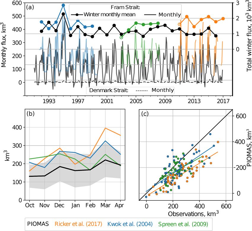
480                                                                V. Selyuzhenok et al.: Sea ice and ocean water temperature

for the Greenland Sea region (see green box in Fig. 1). The          to 350 per year, with a median of 90 casts per year. Even
CS2 dataset provides monthly average sea ice thickness on an         fewer profiles are obtained in the Greenland shelf, which
EASE-2 grid with a 25 × 25 km spatial resolution from 2010           is out of the scope of this study. In the ARMOR dataset,
to 2017. Due to limitations of ice thickness retrieval from          the use of satellite information provides a more precise and
satellite altimetry, the CS2 dataset used was limited only to        detailed picture of spatial and temporal variability of ther-
the cold season (October–April). The sea ice concentration           mohaline characteristics than from interpolation of in situ
data, provided along with CS2 thicknesses, was used to de-           profiles alone (as, for example, in the World Ocean Atlas
rive the effective sea ice thickness (Heff ) for the comparison      dataset, https://www.nodc.noaa.gov/OC5/indprod.html, last
with the PIOMAS data. The conversion was performed for               access: 1 December 2019) and adds robustness to the results.
each grid cell:                                                      The oceanic heat fluxes are estimated using currents from the
                                                                     ARMOR dataset with the same spatial and temporal resolu-
Heff = H × C,                                               (1)      tion. The current velocities at various depth levels are ob-
where H is CS2 sea ice thickness and C is sea ice concentra-         tained by extrapolating the sea surface current from satellite
tion.                                                                altimetry, downwards using the thermal wind relations. The
   Uncertainties in CS2 ice thickness increase below 78◦ N           vertical density profiles, used for the computations, are as-
due to sparse orbit coverage (Ricker et al., 2014). The CS2          sessed from the previously obtained temperature and salinity
retrieval is based on sea ice freeboard measurements that are        profiles (Mulet et al., 2012).
converted into sea ice thickness assuming hydrostatic equi-
                                                                     2.4    Long time series of water temperature of the West
librium. Estimates of snow depth, required for the conver-
                                                                            Spitsbergen Current
sion, are based on the modified Warren climatology (Warren
et al., 1999; Ricker et al., 2014). This climatology is not de-      Long-term monthly gridded water temperatures were ob-
fined in the Fram Strait or Greenland Sea; therefore, snow           tained from “The Climatological Atlas of the Nordic Seas
depth estimates are extrapolated. Moreover, interannual vari-        and Northern North Atlantic” (Korablev et al., 2007). The
ability in snow depth is not captured by the climatology,            database merges together data ICES (International Coun-
which can potentially cause biases in the final sea ice thick-       sel for Exploration of the Sea), from IMR (Institute of Ma-
ness retrieval. High drift speeds can also cause biases in the       rine Research), and from a number of international projects
ice thickness retrieval due to the timing of satellite passes        (ESOP, VEINS, TRACTOR, CONVECTION, etc.), as well
within 1 month. The typical uncertainty is in the range of           as from Soviet Union era cruises in the study region. Since
0.3–0.5 m but may potentially reach higher values.                   there are too few observations in the EGC before the 2000s,
                                                                     we use long-term temperature time series in the upper WSC
2.3   ARMOR dataset
                                                                     (West Spitsbergen Current) at 78◦ N, west of East Fjord
The long-term time series of water temperature at different          (Fig. 1b), an area that is much better sampled. The depth-
depth levels and the mixed-layer depth (MLD) were derived            averaged water temperature at 100–200 m is used, as this
from the ARMOR dataset (http://marine.copernicus.eu/, last           layer is dominated by the AW and is not directly affected
access: 1 December 2019, 1993–2015). The dataset com-                by heat exchange with the atmosphere year-round. This re-
bines in situ temperature and salinity profiles with satellite       sults in the highest temperature at these depths during the
observations and is constructed as follows. First, based on          cold season. Even this region was sampled in a quite irregu-
a joint analysis of the variations in satellite-derived anoma-       lar manner, with a lower sampling frequency in winter. Since
lies (sea surface temperature and sea level from satellite al-       1979, the average number of samples was 161 per year, vary-
timetry) and of in situ thermohaline characteristics at differ-      ing from, on average, 2–5 per year from November to May
ent depths, linear multiple regressions are obtained. The re-        to 20–35 per year from June to October. The data gaps in the
gressions allow for extrapolating satellite data from the sea        time series were filled in by kriging with a 30 km window.
surface to standard oceanographic depth levels in a regu-            The interannual variations presented in this study were aver-
lar mesh of 0.25◦ × 0.25◦ , constructing the so-called “syn-         aged over the months with the densest data coverage (June–
thetic” vertical temperature and salinity profiles. The final        September).
monthly mean 3-D temperature and salinity distributions are
obtained through optimal interpolation of all in situ obser-         3     Methods
vations for this month, together with the derived synthetic
profiles, taken with different weights based on the inverse          3.1    Fram Strait and Denmark Strait sea ice volume
distance and type of measurement (in situ observations were                 flux from PIOMAS
given higher weights) (Guinehut et al., 2012). The number
of in situ vertical temperature profiles in the marginal sea ice     The sea ice volume flux through Fram Strait was calculated
zone (MIZ) area of the Greenland Sea (Fig. 1) is very limited.       as a product of monthly average PIOMAS effective sea ice
Between 1993 and 2016, the number of casts varies from 13            thickness, area of the grid cell and the sea ice drift veloc-

The Cryosphere, 14, 477–495, 2020                                                         www.the-cryosphere.net/14/477/2020/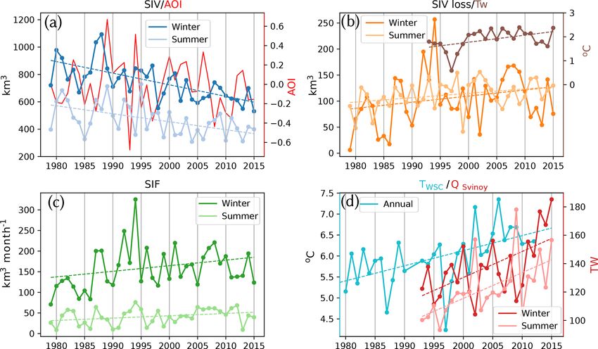
V. Selyuzhenok et al.: Sea ice and ocean water temperature                                                                         481

ity (Ricker et al., 2018). The sea ice drift data were taken         flux of the current month (mth), and t is a time period equal
from the Polar Pathfinder Sea Ice Motion Vectors dataset             to 1 month. The regional sea ice volume was calculated for
(version 3), distributed by the National Snow and Ice Data           the area limited by 82 and 66◦ N latitudes and by the bor-
Center (NSIDC) (Tschudi and Maslanik., 2016). The data are           der in the east, shown in Fig. 1a (green box). We slightly
provided on EASE-2 grid with a 25 × 25 km spatial resolu-            extended the eastern boundary of the Greenland Sea to the
tion. The gate was selected as a combination of a meridional         southeast, compared to its classical definition, in order to in-
section (82◦ N and 12◦ W–20◦ E) and a zonal section (80.5–           clude the entire area of the Odden ice tongue formation. The
82◦ N and 20◦ E), as suggested by Krumpen et al. (2016)              mass balance shows month-to-month increase or loss in sea
(Fig. 1a). The location of the meridional gate at 82◦ N was          ice volume within the Greenland Sea due to sea ice forma-
chosen to reduce biases and errors in sea ice drift that become      tion or melt. Positive MB values correspond to sea ice for-
larger with increasing velocities south of the gate (Sumata          mation and negative values correspond to sea ice melt within
et al., 2014, 2015). The meridional and zonal sea ice volume         the region. The monthly MB values were averaged over an-
flux, Qv and Qu correspondingly, were computed as follows:           nual, winter and summer periods. Note that, due to averaging,
                                                                     negative annual values (sea ice volume loss, Fig. 4) can occur
Qv = l/ cos(λ) × H × (Dx × sin(λ) − Dy × cos(λ)),             (2)    due to both an increase in sea ice melt and a decrease in sea
Qu = l/ cos(λ) × H × (Dx × cos(λ) − Dy × sin(λ)),             (3)    ice formation.

where l = 25 km is the distance between two data points, H           3.3   Mixed-layer depth (MLD) and marginal ice zone
is the PIOMAS effective sea ice thickness, Dx and Dy repre-                (MIZ) ocean temperature
sent sea ice drift velocity in the x and y directions of the grid,
respectively, and λ is the longitude of the respective grid cell.    The MLD was derived using vertical profiles from the AR-
   The total sea ice volume flux through Fram Strait (QF ,           MOR dataset via the method of Dukhovskoy (Bashmach-
positive into the Greenland Sea) was obtained as a sum of            nikov et al., 2018, 2019). The method is similar to that used
the meridional and zonal fluxes along the gate:                      by Pickart et al. (2002) but is applied to the vertical profiles of
                                                                     the potential density gradients. Before processing, the small-
QF = Qu + Qv .                                                (4)    scale noise in the potential density profiles was filtered out
                                                                     with 10 m sliding means. The gravitationally unstable seg-
   The total sea ice volume flux through Fram Strait was de-         ments were artificially mixed to neutral stratification. The
rived for the period from 1979 to 2016 for each month. A             MLD is defined as the depth where the vertical density gra-
similar methodology was used to assess the sea ice volume            dient exceeds its two local standard deviations within a 50 m
flux through Denmark Strait (QD) along the meridional sec-           window, centered at the tested depth (see Bashmachnikov
tion (66◦ N and 35–20◦ W). The positive sign of QD corre-            et al., 2018). The visual control shows that the results are
sponds to a sea ice volume outflow from the Greenland Sea.           mostly similar to the widely used methods by de Boyer Mon-
   In order to assess the data quality, the resultant sea ice vol-   tégut et al. (2004) and Kara et al. (2003), except for weakly
ume fluxes through Fram Strait gate at 82◦ N were intercom-          stratified areas where the Dukhovskoy’s method defines the
pared against available observation-based estimates in the           MLD with higher accuracy. The obtained mean distribution
Fram Strait (Kwok et al., 2004; Spreen et al., 2009; Ricker          of the MLD and seasonal and interannual variations in the
et al., 2018). The gate and the methodology used here were           MLD in the central Greenland Sea are consistent with ob-
adopted from Ricker et al. (2018), while in the other two            servations (Våge et al., 2015; Latarius and Quadfasel, 2016;
studies somewhat different methodologies and gate locations          Brakstad et al., 2019). All the results show an increase in the
(Fig. 1a) were used. Each of the studies is also based on dif-       convection depth from the mid-1990s to the 2000s. There are
ferent datasets of sea ice concentration (SIC), thickness (SIT)      some minor differences in the absolute values of MLD that
and drift (SID) (Table 1).                                           arise from the use of different datasets (e.g., Latarius and
                                                                     Quadfasel, 2016 used only Argo floats) and methodologies
3.2   Greenland Sea sea ice mass balance
                                                                     for MLD detection. These minor differences have not broken
In order to analyze the sea ice volume lost or gained due to         the tendency of the maximum winter MLD to increase since
local melt or freezing, we calculated the sea ice mass balance       the mid-1990s.
(MB) in the Greenland Sea. It was derived for each month                The position of the real MIZ strongly varies in time and
from 1979 to 2016 as follows:                                        along the EGC, being a function of local direction and in-
                                                                     tensity of sea ice transport by wind and current, variation in
MB = (Vm − V(m−1) ) × t − (QFm − QDm ) × t,                   (5)    the characteristics of ice transport from the Arctic, interac-
                                                                     tion of ice floes, local ice thermodynamics, etc. Presence of
where Vm and V(m−1) are regional sea ice volume of the cur-          melting sea ice, in turn, affects the upper-ocean and air tem-
rent month (mth) and the previous month ((m − 1)th), QFm             peratures. A warmer winter ocean warms up the air, which
and QDm are Fram Strait and Denmark Strait sea ice volume            can further be advected over the sea ice causing its melt away

www.the-cryosphere.net/14/477/2020/                                                           The Cryosphere, 14, 477–495, 2020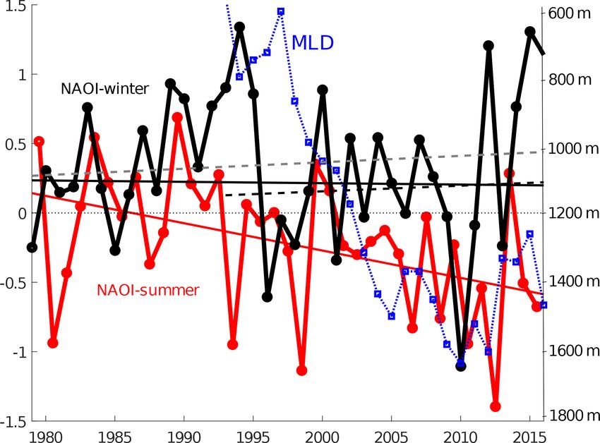
482                                                                      V. Selyuzhenok et al.: Sea ice and ocean water temperature

Table 1. The list of data sources used for estimates of sea ice volume flux through Fram Strait: sea ice concentrations (SIC), sea ice thicknesses
(SIT), sea ice drift velocities (SID) and the time periods of the estimates.

        Study                   SIC                                       SIT                SID                                  Period
        Kwok et al. (2004)      ULS moorings                              ULS moorings       Kwok and Rothrock (1999)        1991–2002
        Spreen et al. (2009)    ASI AMSR-E                                ICESat             IFREMER                         2003–2008
        Ricker et al. (2018)    OSI SAF SIC + sea ice type product        AWI Cryosat-2      OSI SAF                         2010–2017
        this study              –                                         PIOMAS             NSIDC Pathfinder v3             1979–2017

from the sea ice edge. Furthermore, an anomalously warmer                  4     Results
ocean may prevent (or delay) formation of new ice. All these
factors certainly affect the MIZ position. However, if we esti-            4.1    Assessment of PIOMAS-derived ice volume flux
mate ocean temperature variations only along the actual MIZ,                      through Fram Strait and sea ice volume in the
we do not account for these effects. The considerations above                     Greenland Sea
show that defining the oceanic region directly and indirectly
affecting the sea ice volume are not straightforward. In this              In order to assess the quality of the PIOMAS data, monthly
study we examine interannual variations in ocean tempera-                  effective sea ice thickness in the Greenland Sea was com-
ture in a fixed region, which is defined as an area enclosed be-           pared to that derived using the CS2 dataset (Fig. 2). In
tween the 500 m isobath, marking the Greenland shelf break,                general, PIOMAS underestimates effective sea ice thickness
and the mean winter location of the sea ice edge (Fig. 1).                 compared to CS2 (Fig. 1b). The mean difference between PI-
Using the fixed region also assures compatibility of interan-              OMAS and CS2 grid cell values is −0.70 m. There are only
nual temperature variations. For the computations, the sea                 two locations where PIOMAS shows thicker ice compared
ice edge was defined as the 15 % mean winter NSIDC sea ice                 to CS2 north of Spitsbergen and along the sea ice edge. On
concentration for 1979–2016. For brevity, we further, some-                the other hand, CS2 also tends to overestimate sea ice thick-
what deliberately, call this region the MIZ area. Further, we              ness in the marginal ice zone (Ricker et al., 2017). The high-
will see that temperature trends remain positive and of the                est absolute differences between the datasets are attributed to
same order of magnitude all over the western Greenland Sea,                the areas along the Greenland coast (dark blue) and north of
except for a few limited areas along the shelf break. This as-             Spitsbergen (dark red) (Fig. 1b). The monthly scatter plots
sures the robustness of the results regarding the choice of the            (Fig. 2a–g) show that PIOMAS tends to overestimate thin
study region.                                                              sea ice and underestimate thick sea ice thickness, which is in
                                                                           agreement with the tendency reported for the central Arctic
3.4   Oceanic horizontal heat flux                                         (Schweiger et al., 2011). This results in moderate correla-
                                                                           tions between the two datasets (0.63 < r < 0.77) for all win-
The ARMOR data were used to derive a time series of                        ter months. The major discrepancies correspond to sea ice of
oceanic heat flux into the Nordic Seas. Total oceanic heat                 3 m and higher thickness, which form “tails” to the lower-
flux through the Svinøy transect (QSvinøy ) is calculated by               right corner of the scatter plots (Fig. 2a–g).
integrating the heat flux values in the grid points:                          PIOMAS sea ice volume flux through Fram Strait (Octo-
           Z Z                                                             ber to April) was cross-compared with the fluxes derived us-
QSvinøy =        [ρ × cp (T − Tref ) × v]dx dz ,          (6)              ing observation-based sea ice thickness data (see Table 1).
                                                                           The analysis shows that PIOMAS-based sea ice volume flux
                                                                           is in good agreement with the estimates from other datasets
where ρ = 1030 kg m−3 is the mean sea water density, cp =
                                                                           (Fig. 3, Table 2). The correlation coefficients between the
3900 J kg−1 ◦ C−1 is specific heat of sea water, T is sea water
                                                                           three datasets and PIOMAS are over 0.6. The highest cor-
temperature, Tref = −1.8 ◦ C is the “reference temperature”
                                                                           relation of over 0.8, with the Ricker et al. (2018) data, can
and v is current velocity perpendicular to the transect. The
                                                                           be explained by using identical gates and methodology for
reference temperature was set to sea ice melt temperature in
                                                                           estimating ice volume fluxes (Fig. 1a). However, other statis-
order to investigate the contribution of ocean heat fluxes to
                                                                           tical criteria (bias; relative percentage difference, RPD; and
sea ice melt.
                                                                           root-mean-square error, RMSE; see Table 2) indicate a some-
                                                                           what stronger mismatch between the PIOMAS and Ricker
                                                                           et al. (2018) estimates compared to those between PIOMAS
                                                                           and Kwok et al. (2004) or Spreen et al. (2009). The pos-
                                                                           sible sources of this discrepancy are discussed in Sect. 5.
                                                                           Overall, PIOMAS shows lower sea ice volume fluxes com-
                                                                           pared to the observation-based estimates (Fig. 3c). The inter-

The Cryosphere, 14, 477–495, 2020                                                                  www.the-cryosphere.net/14/477/2020/
V. Selyuzhenok et al.: Sea ice and ocean water temperature 483
Figure 2. Density scatter plots of PIOMAS and CS2 monthly effective sea ice thickness (m) in the Greenland Sea, October–April 2010–
2016: (a–g) each point corresponds to one grid cell of sea ice thickness. (h) Mean monthly sea ice thickness over the ice-covered area of the
Greenland Sea for all intercompared snapshots. The colors of the points in panel (h) correspond to a month. The dashed lines show the linear
regression fit and the solid lines are 45◦ angles. The correlation coefficients (r), the slope of the linear regressions and the root-mean-square
error (RMSE) are given in the upper-left corner.
annual variations in the PIOMAS monthly and total winter The reduction of the sea ice volume in the Greenland Sea
sea ice volume flux agree well with other datasets (Fig. 3a; coincides with an increased sea ice volume import through
Table 2). At intra-annual timescales all three datasets show Fram Strait by 9.6 km3 per decade or 8.8 % of its long-term
similar patterns with the minimum flux in October and max- mean (significant at 90 % confidence level). Thus, the total
imum flux in March (Fig. 3b). Overall, moderate to high cor- increase in the sea ice volume imported to the Greenland Sea
relation between the datasets, low relative variance and low through Fram Strait is 115.2 km3 per decade, which accounts
bias (Table 2) suggest that PIOMAS provides a realistic es- for 18.2 % of the Greenland Sea annual mean sea ice volume.
timate of seasonal and interannual variations in the winter The sea ice volume flux through Denmark Strait comprises
sea ice volume flux through Fram Strait. Figures 2h and 3c about 2 % (Fig. 3) of that through Fram Strait and shows no
suggest that PIOMAS correctly captures year-to-year varia- significant tendency. This flux has no considerable effect on
tions in the mean effective sea ice thickness in the Greenland the sea ice mass balance of the Greenland Sea.
Sea and Fram Strait sea ice volume flux. This justifies using A balance between sea ice volume import and export to
PIOMAS for analyzing interannual variations in the integral the Greenland Sea through the straits and regional changes
sea ice volume over the Greenland Sea. in the sea ice volume shows the volume of sea ice formed
or lost due to thermodynamic processes within the region
4.2 Interannual variations in sea ice flux through Fram (Sect. 3.2). The sea ice mass balance in the Greenland Sea,
Strait and sea ice volume in the Greenland Sea expressed in sea ice volume loss, is shown in Fig. 4b. For
about half of the years during the study period, sea ice vol-
ume loss in summer is higher than that in winter. However,
The sea ice volume in the Greenland Sea derived from PI-
there are a few years (1992, 1994, 2004–2007) when winter
OMAS revealed statistically significant (at 99 % confidence
sea ice volume loss significantly exceeds the summer one.
level) negative trends in monthly winter, summer and an-
During these years an increased sea ice volume flux thought
nual values (Fig. 4a, Table 3). The strongest negative trend
the Fram Strait is detected (Fig. 4c). There is a positive statis-
of 84.8 km3 per decade, or 13.5 % of the long-term monthly
tically significant trend in annual and summer monthly mean
annual mean volume, is observed in winter, while for sum-
sea ice volume loss, while the winter trend shows low sta-
mer months the trend was 58.2 km3 per decade or 9.3 % of
tistical significance (Table 3). Overall, the monthly Green-
long-term annual mean volume. The sea ice volume in the
land Sea sea ice volume loss increases by 9.4 km3 per decade
Greenland Sea shows an overall reduction by 72.4 km3 , or
(Fig. 4, Table 3).
11.5 % of its long-term mean per decade.
www.the-cryosphere.net/14/477/2020/ The Cryosphere, 14, 477–495, 2020484 V. Selyuzhenok et al.: Sea ice and ocean water temperature
Table 2. Statistics of monthly PIOMAS versus satellite-based estimates of the sea ice volume fluxes through Fram Strait: Pearson correlation
coefficient (cor. coef.), variance relative to PIOMAS (var. rel.), bias, relative percentage difference (RPD), and root-mean-square error
(RMSE).
Study cor. coef. mean slope var. rel. (%)a biasb RPD (%) RMSE (km3 )
Kwok et al. (2004) 0.70 0.71 98 47 66 75
Spreen et al. (2009) 0.60 0.61 97 33 45 56
Ricker et al. (2018) 0.84 0.66 162 107 88 108
a var. rel. (%) = (100 % · var )/var b
obs PIOMAS . bias = obs. − PIOMAS.
Figure 3. Sea ice volume fluxes (km3 ): (a) time series of PIOMAS and observation-based monthly sea ice volume fluxes through Fram and
the Denmark Straits, 1991–2016 (note that the total winter fluxes are referenced to the right y axis). Empty circles indicate seasons with an
incomplete winter cycle. (b) Winter intra-annual cycle sea ice volume flux through Fram Strait, averaged over the period of the observations
and over 1991–2016 for PIOMAS dataset. The gray background color corresponds to a single standard deviation interval from the PIOMAS
mean. (c) Scatter diagram of monthly mean PIOMAS sea ice volume fluxes through Fram Strait versus monthly mean observations.
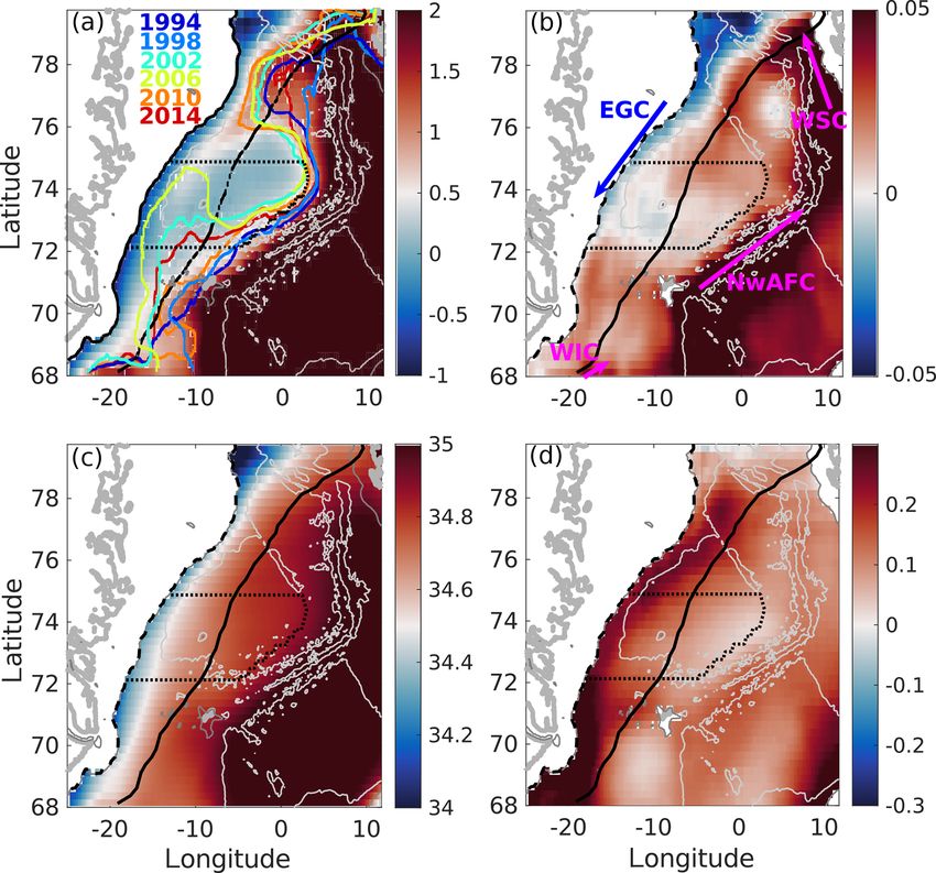
4.3 Interannual variations in water temperature and that the AW should be regularly brought to the ocean surface
MLD in the MIZ of the Greenland Sea by vertical winter mixing, which is consistent with observa-
tions (Håvik et al., 2017; Våge et al., 2018). The presence of
the AW is observed in the climatology, as water temperature
In order to find the reason for the opposite trends in the sea
(and salinity) in the EGC increases with depth, from about
ice volume of the Greenland Sea and the sea ice volume
0 ◦ C near the sea surface to 2–4◦ C at 500 m. In the 24-year
flux through Fram Strait, we investigate water temperature
means, the northern temperature maximum (Fig. 5a) results
in the study region (Sects. 2.3, 3.3, 3.4). A relatively warm
from recirculation of AW of the WSC in the southern Fram
AW is observed in the East Greenland Current (EGC), off the
Strait, while the southern maximum is due to the northwards
Greenland shelf break, below a thin upper mixed layer dom-
heat flux with the North Icelandic Irminger Current (NIIC)
inated by the cold PW. Our estimates of winter MLD show
The Cryosphere, 14, 477–495, 2020 www.the-cryosphere.net/14/477/2020/V. Selyuzhenok et al.: Sea ice and ocean water temperature 485
Table 3. Trends in monthly mean characteristics in the Greenland Sea calculated over annual (September–August), winter (October–April)
and summer (May–September) periods: sea ice volume (SIV, km3 yr−1 ), sea ice volume loss (SIV loss, km3 yr−1 ), sea ice flux through Fram
Strait (SIF Fram, km3 year−1 ), water temperature in MIZ (Tw , ◦ C yr−1 ) and in the West Spitsbergen Current (TWSC, ◦ C yr−1 ), and heat
flux across the Svinøy section (QSvinøy , TW yr−1 ). r 2 is the coefficient of determination, SD is the standard deviation (m) and p value is the
probability value.
Parameter Season Trend r2 SD p value
annual −7.24 (−1.15 %) 0.42 1.48 < 0.01
SIV, km3 yr−1 winter −8.48 (−1.35 %) 0.44 1.66 < 0.01
summer −5.82 (−0.93 %) 0.26 1.72 < 0.01
annual 0.94 (0.88 %) 0.09 0.52 0.08
SIV loss, km3 yr−1 winter 1.18 (1.10 %) 0.06 0.83 0.17
summer 0.84 (0.79 %) 0.10 0.45 0.07
annual 0.96 (0.88 %) 0.09 0.53 0.08
SIF Fram, km3 month−1 yr−1 winter 1.36 (1.25 %) 0.08 0.82 0.10
summer 0.56 (0.52 %) 0.09 0.32 0.08
annual 0.015 (1.50 %) 0.23 0.007 0.04
Tw , ◦ C yr−1 winter 0.008 (0.01 %) 0.05 0.007 0.29
summer 0.026 (3.00 %) 0.29 0.008 < 0.01
annual 1.84 (1.39 %) 0.48 0.41 < 0.01
QSvinøy , TW yr−1 winter 1.83 (1.38 %) 0.35 0.54 < 0.01
summer 1.82 (1.37 %) 0.36 0.53 < 0.01
TWSC , ◦ C yr−1 annual 0.036 (0.60 %) 0.30 0.30 < 0.01
through Denmark Strait (Hansen et al., 2008; Ypma et al., westward propagation is observed in the WSC recirculation
2019). The latter is a northern branch of the Irminger Cur- area (76–78◦ N) and northwest of Jan Mayen (70–73◦ N),
rent. The sea ice is affected by the heat in the upper mixed in the southern Odden tongue region. The tendency of the
layer, the depth of which varies on synoptic, seasonal and isotherm to approach the shelf break is consistent for dif-
interannual timescales. Our analysis shows that the obtained ferent isotherms (from 1 to 3 ◦ C), for different layer thick-
tendencies of increase in water temperature with time, de- nesses (50–200 m) and for different months. Only for winter
rived in the next paragraphs, are largely independent of the months, when the whole upper 200 m mixed layer effectively
choice of the water layer, at least within the upper 200 m of releases heat to the atmosphere, do the interannual trends be-
the water column. In further analysis we present results for come insignificant. The linear temperature trend (Fig. 5b)
the upper 50 m layer (the typical summer mixed layer in the shows warming in the whole area of the eastern MIZ. The
MIZ) and the upper 200 m layer (the typical winter mixed strongest warming follows the pathway of the recirculating
layer in the MIZ, Fig. 6c). In the annual means, the wa- AW in the northern Greenland Sea (Glessmer et al., 2014;
ter temperature, averaged over upper 50 m layer of the MIZ, Håvik et al., 2017), which is known to strongly affect the
has a maximum of 2 ◦ C in September and decreases to 0.1– central regions of the sea (Rudels et al., 2002; Jeansson et al.,
0.2 ◦ C in March–April. Averaged over the upper 200 m, the 2008). The warming in the northern Greenland Sea is linked
patterns of the mean distribution and of (somewhat weaker) to a strong warming of the WSC and the Norwegian Atlantic
tendencies in temperature and salinity closely repeat those Front Current (NwAFC), while that in the southernmost part
in Fig. 5. When averaged over the fixed region, correspond- of the sea is linked with the NIIC. Two exceptions can be
ing to the mean winter MIZ area (Fig. 1), the mixed-layer noted: the northwestern part of the coastally trapped EGC
seawater temperature is always above the freezing point; i.e., (where negative trends are obtained in the area dominated by
overall, the ocean melts sea ice in this area year-round. a colder PW outflow from the Arctic) and the area of the EGC
Figure 5a shows interannual variations in November 2 ◦ C recirculation into the Greenland Sea at 72–74◦ N extended
sea water isotherm (averaged over the upper 200 m layer). from the continental shelf break to 8–9◦ W (here the tenden-
Water temperature in November reflects the heat fluxes accu- cies in the upper-ocean temperature are close to zero). The
mulated during the warm period. It shows the background latter is the area where the Odden ice tongue starts spread-
conditions at the beginning of the winter cooling, when ing into the Greenland Sea interior (Germe et al., 2011). The
sea ice start forming locally. From the 1990s to the 2000s, decreasing temperature in both of these areas is consistent
the 2 ◦ C isotherm approached the shelf break. The largest
www.the-cryosphere.net/14/477/2020/ The Cryosphere, 14, 477–495, 2020486 V. Selyuzhenok et al.: Sea ice and ocean water temperature Figure 4. Time series of winter (December–April) and summer (May–November) and annual ice ocean atmosphere characteristics in the Greenland Sea: (a) monthly mean PIOMAS sea ice volume (SIV, km3 ) and monthly summer AO index (AOI), (b) monthly mean PIOMAS sea ice volume loss (SIV loss, km3 ) and mean September water temperature in MIZ (T w, ◦ C), (c) monthly mean sea ice volume flux through Fram Strait (SIF, km3 month−1 ), and (d) annual mean water temperature in the West Spitsbergen Current (TWSC , ◦ C) and monthly mean ocean heat flux (QSvinøy , TW) through Svinøy section (see Fig. 1). with a stronger sea ice and PW transport from the Arctic (by 0.5 and 0.6◦ C over the 24 years). The winter convection (Sect. 4.2). efficiently uplifts heat to the sea surface. The heat accumu- With a stronger melting of sea ice at the seawards part of lated in summer is mostly released during winter. Figure 4d the MIZ, together with the ice volume loss, we should ob- suggests that the results can be extrapolated back to at least serve a sea ice area loss. This is consistent with Germe et al. 1980, as the slope of the trend lines in temperature of the (2011). In particular, the positive water temperature trend advected AW for 1980–1992 is practically the same as for over the eastern part of the Odden region suggests an overall the period discussed above. We observe a growing difference decrease in the Odden formation by the end of the study pe- between September and March temperatures (Fig. 6a), to- riod. The mean temperature trend over the Odden region (the gether with a decrease in interannual temperature trend to area within the dotted line in Fig. 5b) is 0.08 ◦ C per year, become insignificant in winter. The growing difference in i.e., there is an area-mean increase of 1.8 ◦ C from 1993 to temperature is observed in spite of the equal winter and sum- 2016. This exceeds the mean ocean temperature increase, av- mer trends in the heat inflow with the NwASC (see Tw and eraged in the MIZ area (Eq. 7), which includes the northern QSvinøy in Table 3). Therefore, in the MIZ region, all ad- shelf break regions with negative temperature trends. There- ditional heat accumulated in the upper 200 m layer during fore, the estimates of the heat available for the ice melt, based summer is uplifted to the sea surface by winter convection, on the values presented in Eq.(7), should be considered the preventing ice formation in the ice-free areas or melting the lower limit of the heat release within the Odden region. ice in the ice-covered ones. Interannual variations in water characteristics, averaged In the MIZ, the autumn temperature increases, and the over the upper 200 m and in the MIZ area, are shown in zonal thermal gradient across the MIZ increases by 1.7 times Fig. 6. From 1993, an overall increase in annual mean tem- from 1993 in the annual mean (Fig. 6b) and by nearly 4 times perature in the MIZ is observed, suggesting an increasing in- in winter. This goes along with a decrease in the annual tensity of the sea ice melt. The temperature increases during mean distance between the 2 ◦ C or 3◦ C isotherm and the all seasons, but the strongest increase is detected in autumn shelf break (Fig. 6d): from 120 km in 1993 to 50 km in 2016 The Cryosphere, 14, 477–495, 2020 www.the-cryosphere.net/14/477/2020/
V. Selyuzhenok et al.: Sea ice and ocean water temperature                                                                          487

Figure 5. Marginal sea ice zone (enclosed in black lines) and thermohaline water properties averaged in the upper 50 m layer during the
cold season (October–April). (a) Time-mean (1993–2016) temperature (◦ C) in MIZ and location of 2◦ C isotherm in November for selected
years; (b) linear temperature trend (◦ C yr−1 ) in the upper 50 m-layer from 1993 to 2016; (c) time-mean (1993–2016) salinity in MIZ; (d)
linear salinity trend in the upper 50 m layer from 1993 to 2016. In panel (b), EGC is the East Greenland Current, NwAFC is the Norwegian
Atlantic Front Current, NIIC is the North Icelandic Irminger Current and WSC is the West Spitsbergen Current. Dotted lines in panels (b)
and (d) mark the region where Odden tongue is observed.

(see also Fig. 5a). The direct result of this is a faster melt         ing the ice in the MIZ. The increase in MLD results from
of the sea ice episodically advected from the MIZ eastwards            a higher upper-ocean density due to increasing salinity of
by EGC filaments and mesoscale eddies (Kwok, 2000; von                 the AW, tempered by the increasing temperature (Fig. 5b, d),
Appen et al., 2018). These processes can transport sea ice             which is consistent with the findings of Lauvset et al. (2018).
dozens of kilometers eastward (von Appen et al., 2018). The            Given the increase in ocean temperature in the upper 200 m
most favorable conditions for eddy formation are observed              layer in the MIZ from 1.3 ◦ C in September 1993 to 1.8◦ C in
during northerly winds. The eddies sweep sea ice and PW                September 2016 together with an increase in the mean winter
seawards and advect warm AW closer to the ice edge, result-            MLD from 130 m in 1993 to 180 m in 2016, we can make a
ing in increased bottom and lateral sea ice melt (Bondevik,            rough estimate of the increase (over the 24 years) in the heat
2011). However, a few episodic observations of the ice dy-             released by winter MLD in the MIZ:
namics in the MIZ do not presently allow for quantifying the
importance of this effect.                                             dQ = dQ2016 − dQ1993 = cp × ρwater
   The 24-year mean winter mixed-layer depth (MLD) in                      × (1.8 × 180 − 1.3 × 130) × MIZ area,                     (7)
the MIZ off the Greenland shelf varies from 120 to 250 m,
with the mean value around 150 m, as derived from AR-                  where cp = 3900 J ◦ C−1 kg−1 , ρwater = 1030 kg m−3 and the
MOR dataset. Averaged over the MIZ, MLD increases from                 MIZ area is estimated as 2.3 × 10¹¹ m2 . The computations
the mean value of 130 m in 1993 to around 180 m in 2016                give an additional heat release of 1.5 × 10²⁰ J, following the
(Fig. 6c). Since winter mixing does not reach the lower limit          observed water temperature seasonal cycle, we assume that
of the warm Atlantic water at 500–700 m, the deeper the mix-           all the heat from the growing winter MLD is released at the
ing, the more heat is uplifted towards the sea surface, melt-          sea surface. If all of this heat were to go towards melting the

www.the-cryosphere.net/14/477/2020/                                                             The Cryosphere, 14, 477–495, 2020
488                                                                     V. Selyuzhenok et al.: Sea ice and ocean water temperature

Figure 6. Interannual variations in water properties, averaged over the MIZ area. (a) Temperature drop (◦ C) from maximum in September to
minimum in April next year; (b) annual mean temperature gradient across the MIZ (◦ C km− 1); (c) the mixed-layer depth (m), averaged over
the cold season; (d) annual mean distance of the 3 ◦ C isotherm from the shelf break (km). In panels (a), (b) and (d) the solid black line is the
data averaged over the upper 50 m layer and the dashed gray line is the data over the upper 200 m layer. In panel (d) 3◦ C isotherm is shown
for the 50 m means and 2 ◦ C isotherm for the 200 m means.

ice in the MIZ, we would get an increase in the winter sea ice             5     Discussion
volume loss:
                                                                           5.1    PIOMAS-derived trends
dV = dQ/(L × ρice ) ≈ 500 km3 ,                                   (8)

where the specific heat of ice fusion L = 3.3 × 10⁵ J kg−1                 The revealed regional trends in sea ice volume rely on the PI-
and the ice density of ρice = 920 kg m−3 (Petrich and                      OMAS model data. A comparison of interannual variations
Eicken, 2010). This far exceeds the observed sea ice                       in PIOMAS regional sea ice thickness and the sea ice volume
volume loss in the region (SIV loss monthly winter                         flux through Fram Strait showed that PIOMAS estimates are
trend ×12 months × 24 years ≈ 200 km−3 ). Certainly, not all               in agreement with the observation-based estimates during the
heat released by the upper ocean in the MIZ area goes to the               recent decades. However, the PIOMAS systematic overesti-
ice melt. An unknown fraction of heat is directly transferred              mation of thin ice and underestimation of thick ice thickness,
to the atmosphere through open water, ice leads or is ad-                  reported for the central Arctic, affects the long-term volume
vected away from the MIZ area by ocean currents and eddies.                trend (Schweiger et al., 2011). Schweiger et al. (2011) con-
The sea ice melt may additionally increase haline stratifica-              clude that the PIOMAS-based volume trend is lower than
tion at the lower boundary of the ice, preventing ocean heat               the actual one. Given that similar systematic errors in ef-
from reaching the ice cover. However, the estimates above                  fective sea ice thickness are found for the Greenland Sea
suggest that the autumn warming of the upper MIZ region,                   (Fig. 2), it is likely that the derived Greenland Sea sea ice
limited from below by the winter mixed layer, is able to re-               volume trend is underestimated. The PIOMAS Fram Strait
lease more than enough heat to account for the observed re-                sea ice volume flux can also be affected by these systematic
duction of sea ice volume in the region.                                   errors. The model studies show three major positive peaks in

The Cryosphere, 14, 477–495, 2020                                                                  www.the-cryosphere.net/14/477/2020/
V. Selyuzhenok et al.: Sea ice and ocean water temperature 489
the Fram Strait sea ice volume flux since 1979: 1981–1983, The atmospheric heat convergence over the Greenland Sea
1989–1990, 1994–1995 (Arfeuille et al., 2000; Lindsay and is estimated as the sum of atmospheric heat fluxes across
Zhang, 2005). The anomaly in 1989–1990 was caused by an the northern, southern, eastern and western boundaries of the
increase in the thickness of the transported sea ice, while Greenland Sea (positive fluxes are in the study region), using
the anomaly in 1994–1995 was due to an intensification of ERA-Interim reanalysis. On average, from October to April
southward sea ice drift (Arfeuille et al., 2000). The reduction of following year, we obtained always negative atmospheric
of Arctic multiyear ice fraction during the late 1980s–early heat convergence over the Greenland Sea (1000 to 900 GPa)
1990s (Comiso, 2002; Rigor and Wallace, 2004; Yu et al., of −120 TW on average, varying from −170 to −90 TW. The
2004; Maslanik et al., 2007) are in line with this finding. sign is consistent with typical winter winds from the Arctic
The sea ice volume flux through Fram Strait derived from or Greenland (see, for example, Germe et al., 2011), being
PIOMAS shows the peaks in 1981–1985 and 1994–1995 but warmed while passing over the region. The negative atmo-
does not capture the anomaly of 1989–1990 (Fig. 4c). During spheric heat convergence is roughly balanced by the integral
this period there is no significant shift in the PIOMAS effec- heat release from the ocean to the atmosphere over the same
tive sea ice thicknesses in the Fram Strait, which is likely area on the order of +130 ± 40 TW, assuming the regional
caused by the PIOMAS systematic errors that smoothed the mean winter heat release by the ocean of 150 ± 50 W m−2
differences in thickness between thick and thin ice. Since (Moore et al., 2015).
1993, the PIOMAS Fram Strait sea ice volume flux corre- The heat convergence has tendency to decrease in absolute
lates well with the observation-based fluxes (Fig. 3). The value from 1993 to 2016 by about 4 TW, accompanied by a
main sources of relative errors between the Fram Strait vol- rise of the area-mean winter air temperature of about 1 ◦ C.
ume flux estimates can be related to the different choice of The oceanic southwards heat advection through 77.5◦ N in
methodologies, datasets and gates used to derive sea ice vol- the upper 200 m layer increases by 1 TW. The source of the
ume fluxes (Table 1, Fig. 1). Lower PIOMAS-based sea ice atmospheric warming possibly lies in the northwest, in the
volume flux can be attributed to the above-discussed general southeastern Fram Strait, a known region of high oceanic
PIOMAS tendency to underestimate sea ice thickness. Fig- heat flux into the atmosphere (see, for example, Dukhovskoy
ure 1b shows that for the entire meridional 82◦ N gate, which et al., 2006).
is the main gate for sea ice import to the Greenland Sea, the We argue that at least the overall sea ice volume loss from
PIOMAS effective sea ice thickness is lower compared to the 1993 to 2016 is governed by the ocean. The surplus of the
CS2 effective thickness. In addition, the NSIDC sea ice drift amount of the heat, released by the ocean at the end of the
shows lower speed compared to the OSI SAF drift used in study period, is more than twice of that necessary for bring-
Ricker et al. (2018). A combination of lower drift speed with ing up the observed sea ice volume loss, even when account-
thinner ice thickness might be the reason of the largest offset ing for the detected increase in the sea ice volume import
(Table 2, Fig. 3) between the PIOMAS-based Fram Strait sea through Fram Strait. Heat loss to the atmosphere and the
ice volume fluxes and those derived in Ricker et al. (2018). neighboring ocean areas should take up the rest of the heat.
In particular, the observed increase in ocean temperature over
the Greenland Sea (Fig. 5b) may be a reason for a corre-
5.2 Link to the variability of ocean temperature and
sponding increase in the air temperature, used for explaining
atmospheric forcing
negative trends in the sea ice area (Comiso et al., 2001).
The observed trends are due to both the increase in tem-
The revealed decrease in sea ice volume in the Greenland perature of the AW in the MIZ and an increase in winter
Sea goes in parallel with an increase in the ice volume in- MLD in the area, bringing more AW to the surface. A sig-
flow through Fram Strait. As the sea ice volume flux through nificant vertical extent of the warm subsurface AW layer, go-
Denmark Strait does not show any significant change, this in- ing down to 500–700 m depth (Håvik et al., 2017), results
dicates a simultaneous intensification of the processes of ice in a higher ocean heat release for a stronger mixing for the
melt and reduction in sea ice formation in the sea. The lat- observed MLD in the MIZ. A similar mechanism was sug-
ter is supported by the highest negative trends in the sea ice gested for the Nansen Basin of the Arctic Ocean, where an
area (Fig. 1, expressed in SIC trend) in the area of the Odden enhanced vertical mixing through the pycnocline is thought
tongue between 73 and 77◦ N. to decrease the sea ice area in the basin (Ivanov and Repina,
The interannual variations in sea ice area were previously 2018).
linked to variations in air temperature (Comiso et al., 2001). In turn, the subsurface AW in the EGC is fed by the re-
The results of our paper permitted us to speculate that ocean circulation of the surface water of the WSC, an extension
temperature may be important in controlling Odden forma- of the Norwegian Atlantic Front Current (NwAFC) and the
tion (see also Shuchman et al., 1998; Germe et al., 2011). Norwegian Atlantic Slope Current (NwASC). The recircula-
For example, the reduction of Odden tongue occurrence in tion is mostly driven by eddies (Boyd and D’Asaro, 1994;
the 2000s (Latarius and Quadfasel, 2010) might be partially Nilsen et al., 2006; Hattermann et al., 2016). The interan-
driven by the increase in upper-ocean heat content (Fig. 5b). nual variations in the vertical mixing intensity between the
www.the-cryosphere.net/14/477/2020/ The Cryosphere, 14, 477–495, 2020490 V. Selyuzhenok et al.: Sea ice and ocean water temperature AW, the PW and the modified AW, returning from the Arc- The intensity of the flux may be damped by nonlinear depen- tic through the southern Fram Strait, as well as variations dence due to the AW entering the recirculation as eddy shed- in ocean–atmosphere exchange in that area, leads to inter- ding. Additionally, observations demonstrate that the posi- annual variability of the AW advected by the EGC into the tive NAO phase drives a stronger ice drift through Fram Strait Greenland Sea (Langehaug and Falck, 2012). All the pro- (Vinje and Finnekåsa, 1986; Koenigk et al., 2007; Giles et al., cesses intensify during highly dynamic winter conditions. 2012; Köhl and Serra, 2014), a stronger EGC (Blindheim Nevertheless, interannual correlation of the summer upper- et al., 2000; Kwok, 2000) and a typically larger extension ocean water temperature (0–200 m), spatially averaged over of Odden ice tongue (Shuchman et al., 1998; Germe et al., the MIZ area, with that in the upper WSC is 0.8–0.9. Further 2011). The stronger PW transport also dams the AW anoma- south, correlation of interannual variations in the MIZ tem- lies, entering into the study region. perature with that of the NwAFC (NwASC) or with the heat NAO phase is shown to be the main driver for interan- flux across the Svinøy section are low. The decrease is due nual variations in sea ice volume flux to the Greenland Sea to damping of the advected heat anomalies in the Norwegian (Germe et al., 2011; Ricker et al., 2018). The simultaneous Sea by eddy heat transport and ocean–atmosphere exchange long-term (1974–1997) intensification of the AW inflow in (Asbjørnsen et al., 2019). Besides differences in local forc- the Nordic Seas across the Faroe–Shetland Ridge and of east- ing, regional atmospheric forcing over the northwestern Bar- wards advection of PW to the southwestern Norwegian Sea, ents Sea regulates the interannual variations in the heat redis- as a response to NAO forcing, has been noted in several stud- tribution between the WSC and the Barents Sea (Lien et al., ies (see, for example, Blindheim et al. (2000); Yashayaev and 2013), further decreasing the correlations. Seidov (2015). Nevertheless, in the long run (over the four most recent From the beginning of the 1970s, the winter NAO index decades), temperature at the WSC, the NwAFC, NwASC has been growing. From 1979 to 2016 it was mostly positive and the heat flux across Svinøy section all show positive (Fig. 7), although an overall winter trend can be separated trends (Figs. 4, 5). This is confirmed by a number of stud- into an increase from 1979 to 1994, a rapid drop from 1995 ies (Alekseev et al., 2001b; Piechura and Walczowski, 2009; to 1996 and an increase from 1996 to 2016. The NAO in- Beszczynska-Möller et al., 2012). The trends form a part of dex drop in 1995–1996 coincides with a drop in regional sea the long-term oscillation of water temperature in the Norwe- ice volume loss and a decrease in the WSC water tempera- gian Current (Yashayaev and Seidov, 2015). ture (Fig. 4b, d). This can be related to the minimum heat Pressure fields in the northern North Atlantic are mainly flux through the Svinøy section in 1994 (Fig. 4d). The time governed by NAO and the East Atlantic patterns (Woollings needed for water properties to propagate from Svinøy to the et al., 2010; Moore and Renfrew, 2012; Foukal and Lozier, Fram Strait with the NwASC is on the order of 1.5–2 years 2017). Both patterns affect the wind stress curl, largely reg- (Walczowski, 2010). ulating ocean circulation in the Nordic Seas. During the pos- Summer NAO index does not govern the interannual vari- itive NAO phase, the cyclonic atmospheric circulation over ations in the atmospheric or oceanic systems (circulation in the Nordic Seas intensifies (Skagseth et al., 2008; Germe the Nordic Seas intensifies in winter and is thought to bring et al., 2011). This leads to stronger northerly winds along the more AW to the recirculation region compared to that in sum- Greenland shelf, as well as stronger southerly winds along mer). Consistent with other studies of seasonal interannual the Norwegian coast, which results in a more intensive cy- variations in current intensity in the region, our results sug- clonic oceanic circulation in the Nordic Seas (Schlichtholz gest that these are winter variations in the AW transport that and Houssais, 2011). Several regional studies, based on in bring up the interannual variations in the subsurface water situ data, demonstrate a higher intensity of oceanic trans- temperature in the MIZ of the Greenland Sea. The decreas- port of volume and heat along the AW path towards the Fram ing summer NAO index from 1979 may be responsible for a Strait during the positive NAO phase (Raj et al., 2018; Wal- somewhat stronger tendency in the SIV loss in winter com- czowski, 2010; Chatterjee et al., 2018). Thus, change from pared to summer (Fig. 4a, b). strongly negative to strongly positive NAO index (NAOI) re- Summing up, the positive phase of NAO intensifies the sults in an increase by 50 % of the NwASC transport as well whole current system of the Nordic Seas, simultaneously in- as increasing the oceanic heat flux (Skagseth et al., 2004, tensifying sea ice flux through Fram Strait and the northward 2008; Raj et al., 2018). We obtained a significant correlation heat flux with the AW to the Nordic Seas. In this paper we between NAOI and oceanic heat advection with the Norwe- demonstrated that the intensification of the AW heat inflow gian current at Svinøy (0.5 for the heat flux integrated over contributes to variations in the sea ice volume in the Green- the upper 500 m layer). The link between the AW transport land Sea. This supplements previous results, showing that the by the WSC, as well as the cyclonic circulation in the Green- AW inflow dominates the oceanographic conditions over the land Sea, and NAO phase is also obtained from observations upper Greenland Sea, except for the shelf area (e.g., Alek- and numerical models (Walczowski, 2010; Chatterjee et al., seev et al., 2001a; Marnela et al., 2013). 2018). Correlation of NAOI with southward heat flux in the In spite of the stronger ice melt, the upper-ocean salinity Fram recirculation is also positive but not significant (0.3). in MIZ, as well as along the EGC and in the NwASC, has in- The Cryosphere, 14, 477–495, 2020 www.the-cryosphere.net/14/477/2020/
You can also read