Direct measurements of black carbon fluxes in central Beijing using the eddy covariance method - Recent
←
→
Page content transcription
If your browser does not render page correctly, please read the page content below
Atmos. Chem. Phys., 21, 147–162, 2021
https://doi.org/10.5194/acp-21-147-2021
© Author(s) 2021. This work is distributed under
the Creative Commons Attribution 4.0 License.

Direct measurements of black carbon fluxes in central Beijing
using the eddy covariance method
Rutambhara Joshi1 , Dantong Liu1,a , Eiko Nemitz2 , Ben Langford2 , Neil Mullinger2 , Freya Squires3 , James Lee3,4 ,
Yunfei Wu5 , Xiaole Pan5 , Pingqing Fu5 , Simone Kotthaus6,b , Sue Grimmond6 , Qiang Zhang7 , Ruili Wu7 ,
Oliver Wild8 , Michael Flynn1 , Hugh Coe1 , and James Allan1,9
1 School  of Earth and Environmental Science, University of Manchester, Manchester, United Kingdom
2 UK   Centre for Ecology and Hydrology, Penicuik, United Kingdom
3 Department of Chemistry, University of York, York, United Kingdom
4 National Centre for Atmospheric Science, University of York, York, United Kingdom
5 Institute of Atmospheric Science, Chinese Academy of Sciences, Beijing, China
6 Department of Meteorology, University of Reading, Reading, United Kingdom
7 Ministry of Education Key Laboratory for Earth System Modelling, Department of Earth System Science,

Tsinghua University, Beijing, China
8 Lancaster Environment Centre, Lancaster University, Lancaster, UK
9 National Centre for Atmospheric Science, University of Manchester, Manchester, United Kingdom
a now at: Department of Atmospheric Sciences, School of Earth Sciences, Zhejiang University,

Hangzhou, Zhejiang, 310027 China
b now at: Institut Pierre Simon Laplace, École Polytechnique, Palaiseau, France

Correspondence: James Allan (james.allan@manchester.ac.uk) and Rutambhara Joshi (joshi.rutambhara@gmail.com)

Received: 23 June 2020 – Discussion started: 15 July 2020
Revised: 6 November 2020 – Accepted: 6 November 2020 – Published: 8 January 2021

Abstract. Black carbon (BC) forms an important component         are also larger (factor of 37.5 in winter and 37.7 in summer)
of particulate matter globally, due to its impact on climate,    than the measured flux. Emission ratios of BC / NOx and
the environment and human health. Identifying and quanti-        BC / CO are comparable to vehicular emission control stan-
fying its emission sources are critical for effective policy-    dards implemented in January 2017 for gasoline (China 5)
making and achieving the desired reduction in air pollution.     and diesel (China V) engines, indicating a reduction of BC
In this study, we present the first direct measurements of ur-   emissions within central Beijing, and extending this to a
ban BC fluxes using eddy covariance. The measurements            larger area would further reduce total BC concentrations.
were made over Beijing within the UK-China Air Pollu-
tion and Human Health (APHH) winter 2016 and summer
2017 campaigns. In both seasons, the mean measured BC
mass (winter: 5.49 ng m−2 s−1 , summer: 6.10 ng m−2 s−1 )        1   Introduction
and number fluxes (winter: 261.25 particles cm−2 s−1 , sum-
mer: 334.37 particles cm−2 s−1 ) were similar. Traffic was de-   Particular matter with a diameter ≤ 2.5 µm (PM2.5 ) is a ma-
termined to be the dominant source of the BC fluxes mea-         jor contributor to air pollution (Harrison et al., 1997). It
sured during both seasons. The total BC emissions within the     is a global concern given its severe impacts on health, as
2013 Multi-resolution Emission Inventory for China (MEIC)        epidemiological studies identify a variety of cardiovascular
are on average too high compared to measured fluxes by a         and respiratory diseases (Lelieveld et al., 2015; Pope and
factor of 58.8 (winter) and 47.2 (summer). Only a compar-        Dockery, 2006). The daily recommended exposure limit of
ison with the MEIC transport sector shows that emissions         PM2.5 suggested by the World Health Organisation (WHO)
                                                                 is 25 µg m−3 (Jassen et al., 2012). However, in China con-

Published by Copernicus Publications on behalf of the European Geosciences Union.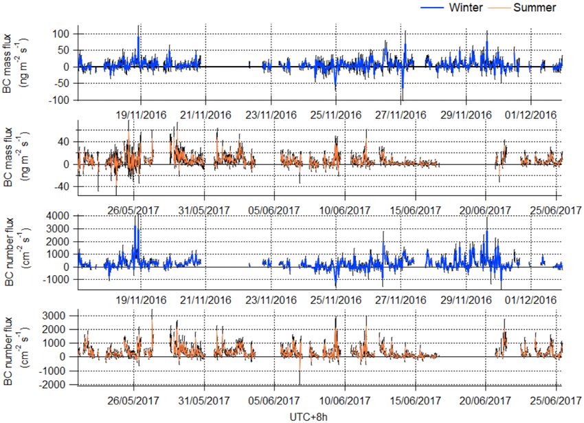
148                                            R. Joshi et al.: Direct measurements of black carbon fluxes in central Beijing

centrations routinely are on the order of 100s µg m−3 (Li et        2018). EC allows for the direct measurement of the magni-
al., 2017; Zhang et al., 2017; Zíková et al., 2016). Black car-     tude of the net flux from the upwind area or the flux foot-
bon (BC), in general, contributes up to 10 %–15 % of overall        print (up to a few kilometres, depending on measurement
PM2.5 and is emitted from incomplete combustion of fossil           height and meteorological conditions), providing quantifica-
fuel and biofuel (Seinfeld and Pandis, 1998). Even though its       tion of the fluxes at the local scale. This study is part of the
abundance is relatively low in PM2.5 , the WHO reports that         wider UK-China Air Pollution and Human Health (APHH)
a 1 µg m−3 increase in BC is associated with greater health         project, which had field campaigns in Beijing during winter
risks compared to the same increase in unidentified PM2.5           (16 November–10 December 2016) and summer (15 May–
mass (Jassen et al., 2012). Furthermore, BC is the most op-         30 June 2017) (Shi et al., 2019). Also as part of this project,
tically absorbent aerosol in the atmosphere, with radiative         ambient BC concentrations were measured using a separate
forcing to the climate second only to CO2 (Bond et al., 2013;       SP2 connected to a conventional inlet line, as described by
Ramanathan and Carmichael, 2008). Therefore, reducing BC            Liu et al. (2019) and Yu et al. (2020).
will potentially have major benefits for both air quality and
climate.
   The capital of China, Beijing, is well known for its air         2     Method
quality issues, with a large population frequently exposed
                                                                    2.1    Site location
to unsafe levels of air pollution. Therefore, improving air
quality is a priority for government and environmental agen-        During the APHH project, two SP2 instruments were used to
cies in China. Ongoing policies targeting reduction in the          study concentrations and fluxes of BC at the Institute of At-
use of solid fuel domestic cooking and heating (Barrington-         mospheric Physics (IAP; 39◦ 580 2800 N, 116◦ 220 1600 E), sam-
Leigh et al., 2019) and introducing traffic management poli-        pling from an inlet placed on the IAP meteorological tower.
cies and vehicular emission controls (Wu et al., 2017) have         When the tower was built in 1979 for long-term meteoro-
been successful in reducing PM2.5 and consequently BC in            logical and environmental monitoring, it was surrounded by
recent years (Sun et al., 2016). However, Beijing still suf-        croplands. Following rapid urbanisation and industrialisa-
fers from severe haze episodes, with BC concentrations fre-         tion, it is now surrounded by a heterogeneous urban land use
quently 10 times greater than those observed in western             between the 3rd and 4th Ring Roads. This includes a small
countries (Liu et al., 2014; Wu et al., 2016). Therefore, un-       park (∼ 0.3 km2 ) to the west, the Beijing–Tibet Expressway
derstanding and quantifying BC emission sources can help            (∼ 400 m) to the east and a busy road (Beitucheng, crossing
reach the Chinese government targets for clean air.                 from east to west, ∼ 100 m) to the north of the tower.
   Scientists routinely use atmospheric chemistry models to
assess local and regional air quality and determine the effec-      2.2    Instrumentation: SP2
tiveness of potential legislative interventions. As air quality
models are underpinned by emission inventories, the accu-           BC concentrations were measured using an SP2 model B
racy of their forecasts is closely coupled to inventory uncer-      (retrofitted with photomultipliers for incandescence detec-
tainties from emission factors and activity statistics (e.g. fuel   tion and the newer 8-channel data acquisition system) during
consumption and source) (Cao et al., 2006; Hodnebrog et al.,        the winter period and an SP2 model C during the summer
2014). Such uncertainties are challenging to resolve as the         period. As the same calibration and data analysis protocols
spatial resolution increases up to a few kilometres (Zheng et       were followed, no indication of a systematic difference in
al., 2017).                                                         quantification was noted. The Droplet Measurement Tech-
   In China, sources have rapidly changed with urbanisation         nologies (DMT) SP2 (Boulder, Colorado) can quantify the
and environmental controls. Ground-based measurements of            mass of the refractory BC (rBC) within individual aerosol
emissions can help to refine and verify emission inventories.       particles using laser-induced incandescence (LII) without
For BC, this is complicated by the use of BC / PM2.5 ra-            any influence of non-rBC material (Moteki and Kondo, 2007;
tios to estimate BC emissions. This ratio is highly variable        Schwarz et al., 2006). The laser beam operating at 1064 nm
depending on fuel type and combustion conditions (Bond              is used to measure rBC (hereafter referred to as BC) on a sin-
et al., 2004; Streets et al., 2001). Consequently, analysis of      gle particle basis. The laser heats up the particle, causing it to
the physical and chemical properties of BC to help identify         incandesce if BC is present. The intensity of incandescence
source and combustion conditions is essential to better char-       signal is proportional to the mass of the BC, which requires
acterise BC particles.                                              calibration using size-selected soot standards. In this study,
   In this study, we measure BC concentrations using a Single       calibrations for both SP2B and SP2C in the incandescence
Particle Soot Photometer (SP2, DMT, Boulder) and present            channel were performed throughout each campaign using
the first ever source-characterised urban flux measurements         Aquadag® BC particles, to avoid the instrument-based bi-
of BC determined using the micrometeorological eddy co-             ases of SP2B and SP2C. Since Aquadag® has higher sensitiv-
variance (EC) method. To date, EC-measured BC fluxes have           ity to the incandescence channel than ambient BC particles,
only been undertaken for one grassland site (Emerson et al.,        a correction is applied using a multiplication factor of 0.75

Atmos. Chem. Phys., 21, 147–162, 2021                                                  https://doi.org/10.5194/acp-21-147-2021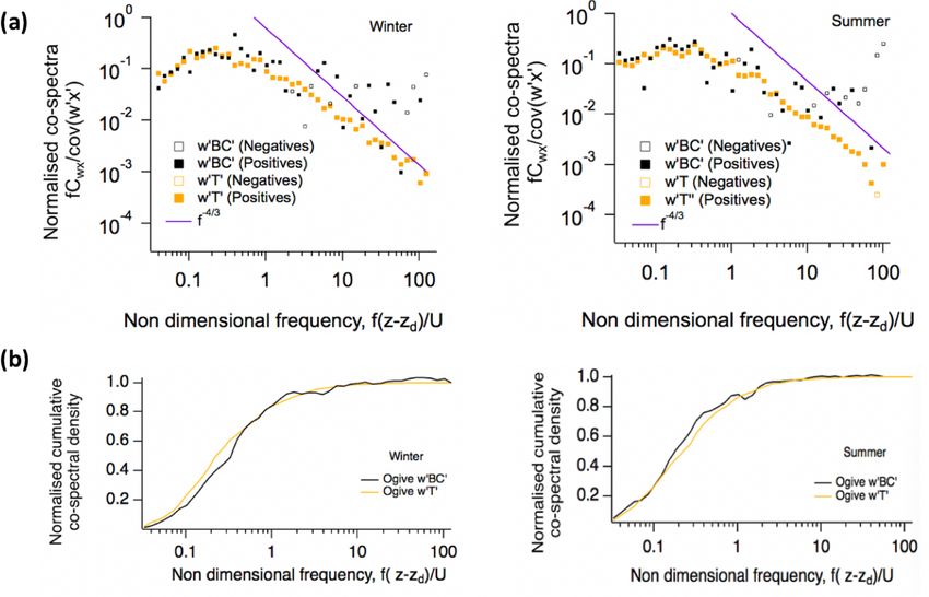
R. Joshi et al.: Direct measurements of black carbon fluxes in central Beijing                                                   149

(Laborde et al., 2012). The mass of BC is then converted to
mass-equivalent diameter using a density of ρ = 1.8 g cm−3
(Bond and Bergstrom, 2006). Here, we use the same termi-
nology as Liu et al. (2014) and refer to the mass-equivalent
diameter as the core diameter (Dc ), which is the diameter of
the sphere containing the same mass of BC as measured in
the particle. The ambient BC is often internally mixed with
other aerosols, often referred to as the “coating”. The over-
all size of the particle can be estimated based on the scat-
tering signal using a “leading-edge-only” (LEO) fit (Gao et
al., 2007). In this study, to quantify the coating content of
a BC particle, we introduce a parameter scattering enhance-
ment (Esca ) in Eq. (1), as discussed by Liu et al. (2014) and
Taylor et al. (2015).

          Smeasured, coated BC
Esca =                                                        (1)    Figure 1. Eddy covariance (EC) measurement setup on the IAP
         Scalculated, uncoated BC                                    tower for BC flux measurements. The aerosol and BC were sam-
                                                                     pled from an inlet placed at 102 m above ground level. The sonic
Here, Smeasured, coated BC is the scattering intensity of the        anemometer 0.75 m from the inlet measured the wind components
coated BC particle measured using SP2 with the LEO fit ap-           and virtual temperature.
plied, and Scalculated, uncoated BC is the scattering intensity of
the uncoated BC based on the measured mass and using a re-
fractive index of BC of nBC = 2.26–2.16i reported by Moteki          turbulent flow profile until just in front of the SP2 and made
and Kondo (2010) for the SP2 wavelength λ = 1064 nm. Esca            AMS and SP2 measurements as consistent as possible.
is proportional to the coating content of a particle, and for           The raw data recorded by the SP2 are the multi-channel
a given particle, if Esca = 1, this suggests that such a parti-      data for individual particles; however only a subset of the
cle has no coating, noting that the precision of the scattering      particles detected is typically recorded, due to limitations im-
measurement and the model used to predict scattering are not         posed by hard drive space and computer throughput. Since
perfect, so this measurement should only serve as a qualita-         we were operating in a heavily polluted environment, we set
tive indicator.                                                      the particle recording frequency to 1 in 30 for winter and 1
                                                                     in 5 for summer. Ideally, every single particle (i.e. 1 in 1)
2.3   Measurement setup                                              would be analysed to maximise counting statistics and min-
                                                                     imise uncertainty in the flux calculation, but limitations in
Figure 1 shows the measurement setup for the EC measure-             data storage and processing power of the built-in computer
ments. A 1/2 in. o.d. copper sampling inlet was placed at            prevented this. Count frequencies were based on the instru-
102 m height. The measurement height is almost 2 times               ment performance and ambient concentrations, with concen-
higher than the mean building height in all but the southerly        trations higher in winter.
direction (Liu et al., 2012), and it is 6 times higher than             During acquisition, the instrument handles data in 200 ms
the mean displacement height. The open lattice triangular            buffers, and each recorded particle is timestamped accord-
cross-section tower structure was designed to minimise dis-          ing to the buffer, so when the data are processed, it pro-
tortion of the air flow. A three-dimensional sonic anemome-          duces number and mass concentrations with a 5 Hz time res-
ter (Model R3-50, Gill Instruments, Lymington, UK) was               olution. If during acquisition a buffer is not fully processed
used during both seasons. The sonic anemometer sampled               before the next one has finished collection (which can oc-
at a frequency of 20 Hz, and it was mounted with a north             cur at high concentrations), then a data buffer is discarded,
offset of 13 and 31◦ during winter and summer measuring              which is manifested as a 200 ms gap in the data. Overall data
periods, respectively. Ambient air was pumped down to the            losses were 7.5 % in winter and 4.2 % in summer. The higher
analysers at ground level, with a flow of ∼ 90 L min−1 . Ad-         losses in winter were because of the higher concentrations
ditionally, at ground level, the sample line was isokinetically      and the fact the SP2-B used an older and lower specification
divided into four flows using a TSI flow splitter. Two ports         logging computer compared to the newer SP-C used in the
were connected to the pump; one was connected to an Aero-            summer. This is in spite of the lower data saving frequency.
dyne aerosol mass spectrometer (AMS), which deployed a               In both seasons, single data gaps were interpolated as they
further bypass pump providing an additional flow of about            were assumed to be due to dropped buffers. Longer gaps
1 L min−1 , and the other pulled air past the SP2 sampling           (symptomatic of other instrument problems) were treated as
inlet at a flow rate of ∼ 1 L min−1 , from which the SP2 sub-        downtime.
sampled at a flow of 0.1 L min−1 . This setup guaranteed the

https://doi.org/10.5194/acp-21-147-2021                                                  Atmos. Chem. Phys., 21, 147–162, 2021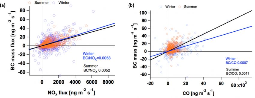
150                                           R. Joshi et al.: Direct measurements of black carbon fluxes in central Beijing

2.4   Black carbon flux calculations                              dent on turbulence generated from wind shear. After sunrise,
                                                                  additional heating (solar, and human activities) can enhance
The EC method derives the net flux of BC through the hori-        turbulence, making it more buoyant. This increase occurs in
zontal plane at the height of the measurement from the corre-     both seasons. This effect is stronger in summer as the ra-
lation between the fluctuations in the measured vertical wind     diation is stronger and the stored heat is greater (Fig. 2b).
speed (w) and BC concentrations, which can be related to          Furthermore, it is crucial to confirm that measurements are
the flux between the surface and atmosphere (Emerson et al.,      within the boundary layer, so they can be related to sur-
2018).                                                            face emissions. The mixed layer heights (MLHs) are derived
          0 ,                                                     from ceilometer (Vaisala CL31, Finland) measurements at
FBC = w0 CBC                                               (2)    the base of the tower using the CABAM algorithm (Kotthaus
where the net BC flux (FBC ) is calculated as the product of      and Grimmond, 2018). In both seasons the average MLH is
the instantaneous fluctuation in vertical wind speed (w 0 ) and   greater than the measurement height (Fig. 2c).
in BC concentration (CBC  0 ), summed over an averaging pe-

riod of 30 min. The fluctuations are derived using Reynolds
                                                                  3     Quality assurance and corrections
decomposition, e.g. w0 = w −w, where the overbar indicates
an arithmetic mean. In the atmosphere, such fluctuations are      3.1    Stability, stationarity and storage corrections
driven by turbulence and have timescales ranging from mil-
liseconds to a few hours. Therefore, the net correlations of      Rural fluxes are often filtered to remove low friction veloc-
these fluctuations are summed over a timescale that is suffi-     ity periods (e.g. u∗ < 0.2 m s−1 ) when vertical exchange is
cient to capture the majority of fluxes, without non-stationary   suppressed, and surface emissions may not reach the mea-
influences from true changes in emission or meteorology.          surement height but may instead be advected (e.g Barr et al.,
   We use the widely used open-source software, EddyPro           2013). For urban flux measurements, given the large stor-
software version 6.2.1 (LI-COR Inc.), to calculate the fluxes     age and anthropogenic heat fluxes, the urban areas may re-
as used with CO2 and other greenhouse gas flux measure-           main unstable (e.g. Kotthaus and Grimmond, 2012, 2014) or
ments. A time lag occurs between wind and BC measure-             not (Ward et al., 2013), making a single cut-off value of u∗
ments from the spatial separation of the sonic anemometer         challenging because, unlike for rural CO2 exchange, times
and the SP2. Time lags can be determined for each 30 min pe-      during which fluxes should be independent of u∗ are diffi-
riod, but they can be difficult to quantify when the measure-     cult to predict. This is due to the complex boundary layer
ments have a low signal-to-noise ratio and fluxes are asso-       behaviour caused by the heterogeneity of the urban canopy,
ciated with higher uncertainty (Langford et al., 2015). Here,     urban heat island effect and release of storage heat to the
time lags are calculated using 24 h periods of 5 Hz data, with    boundary layer. In this study, we applied a filtering thresh-
application of the covariance maximisation method (Nemitz         old of u∗ ≤ 0.15 m s−1 . The data loss from this is higher in
et al., 2008; Su et al., 2004) giving a time lag for each day.    winter (21 %) than summer (13 %). Removing these data in-
As these are found to be consistent, a mean constant time         creases mean BC fluxes; the average mass and number fluxes
lag of 13 (winter) and 14 s (summer) is used. For stream-         increased by 10 % during winter and in summer, and the mass
line corrections, the double rotation method is used with the     and number fluxes increased by 14 % and 13 % respectively.
three velocity components of the anemometer (Wilczak et al.,      Periods of lower turbulence typically occur at night when
2001). Finally, the fluxes were calculated using a linear de-     the MLH is also lower. In those conditions, without efficient
trending method for each 30 min of averaging period but only      transport of emissions to the measurement height, a build-
if the averaging period had missing data gaps that accounted      up in concentration below this level may occur (i.e. positive
for less than 10 % of the data loss. Missing data are caused      storage flux). This build-up is typically released later when
by either interruption in sampling (e.g. instrument mainte-       the boundary layer grows (i.e. negative storage flux). Here, a
nance, calibration) or problems with the logging computer         single-point storage flux correction is calculated as (Rannik
(Sect. 2.2). The random uncertainty in the measurements           and Vesala, 1999)
is calculated following the Finkelstein and Sims (2001) ap-
proach.                                                                  c (t + 1t) − c(t − 1t)
                                                                  Fs =                          × z.                           (3)
                                                                                  21t
2.5   Environmental and micrometeorological conditions
                                                                  Here, Fs is the storage flux term, c is the concentration,
The vertical transport of the BC emitted depends on microm-       z is the measurement height and 1t = 30 min. The storage
eteorology and environmental conditions. The friction veloc-      correction was considered when the surface emission was
ity (u∗ ) is a measure of the efficiency of the vertical trans-   required (e.g. diurnal cycles). For deriving correlations be-
port of momentum and thus also of the pollutants (Fig. 2a).       tween co-emitted pollutants with the BC flux, storage correc-
During the early hours of the day, in the absence of solar        tion is not applied to any of the metrics as this is not required
heating, friction velocities are lowest and are more depen-       and could potentially add additional error. The EC method

Atmos. Chem. Phys., 21, 147–162, 2021                                                https://doi.org/10.5194/acp-21-147-2021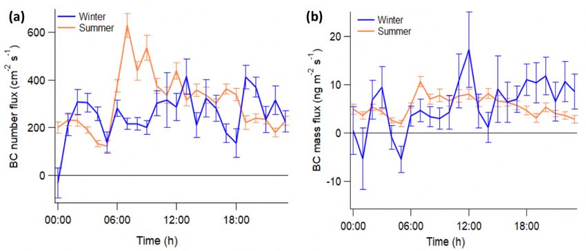
R. Joshi et al.: Direct measurements of black carbon fluxes in central Beijing                                                          151

Figure 2. Winter (blue) and summer (orange) diurnal pattern of (a) friction velocity (u∗ ), (b) sensible heat flux and (c) mixed layer height
(m). Shaded areas are the interquartile ranges, and the solid line is the mean.

assumes steady-state conditions, which is often not satisfied            lapses on the w0 T 0 ogive. During summer, scaling of 0.91 is
due to a change in weather patterns and meteorological vari-             required, resulting in a flux loss of 9 %. In the case of winter,
ables with time of the day. The stationarity test described by           as the w0 BC0 ogive sits below the w0 T 0 ogive, scaling of > 1
Foken and Wichura (1996) is often performed to examine                   required, suggesting the w 0 T 0 spectrum is damped compared
whether a flux is statistically invariant over the averaging pe-         to w 0 BC0 , which is not physically feasible. Generally, this
riod. However, this test is unreliable for small fluxes with             analysis describes the challenges of emulating flux losses in
large uncertainties (e.g Nemitz et al., 2018); therefore this            noisy data, and as the losses are minor, we have not applied
filter is not applied in this study to avoid flagging of averag-         this correction.
ing periods as non-stationary irrespective of meteorological
conditions.
                                                                         4     Results
3.2   Spectral analysis                                                  4.1    Tower and ground comparison

Spectral analysis is a useful approach for diagnosing the na-            The physical properties of BC in Beijing during this cam-
ture of turbulence captured by an EC system (Kaimal et al.,              paign for both seasons have been discussed by Yu et
1972). Generally, power spectra of the measured scalar (x)               al. (2020) and Liu et al. (2019) based on the concurrent
are used to demonstrate an instrument’s response to captur-              ground-level SP2 observations. The mass ratio of internally
ing the range of turbulent fluctuations, but the poor BC count           mixed non-BC material (the “coating”) to BC was quanti-
statistics (Sect. 2.2) resulted in power spectra that resem-             fied by Yu et al. (2020), which varied from 2 to 12 in the
bled white noise (not shown). Instead, the covariance spec-              winter season and 2 to 3 in the summer season. The higher
tra (vertical wind and scalar, w0 T and w0 BC0 ) are shown               variability during the winter was related to a combination of
in Fig. 3. To minimise the effect of outliers in the spec-               frequent occurrences of heavy haze episodes and the pres-
tra, a median is used (Järvi et al., 2014) with instantaneous            ence of additional sources compared to the summer seasons.
fluxes less than 0 ng−2 s−1 (both seasons) and low frictional            Liu et al. (2019) performed source apportionment analysis
velocities (less than 0.25 m s−1 in winter and 0.38 m s−1 in             for the same ambient BC measurements and identified four
summer) removed. BC mass co-spectra show the same co-                    different BC modes, which were then compared with AMS
spectral peak and follow sensible heat co-spectra up to a non-           and SP-AMS measurement to relate each mode to their po-
dimensional frequency of 5, at which the effect of noise be-             tential pollutant source. These four modes were identified
comes visible. This covers that majority of the flux contribu-           using the Esca method described in Sect. 2.2 and include
tion which occurs from lower frequencies. The trend in high              thickly coated (coating diameter, ct > 200 nm); small, thinly
frequency at the inertial subrange range follows the f −4/3              coated (ct < 50 nm and Dc < 180 nm); moderately coated
response as predicted by Kolmogorov theory (Kaimal and                   (50 nm > ct < 200 nm); and large, thinly coated (ct < 50 nm
Finnigan, 1994) (Fig. 3a, purple), which is evident for sen-             and Dc > 180 nm) particles. Their study also suggested that
sible heat flux. The high-frequency flux loss due to atten-              thinly coated particles had a strong association with traffic-
uation was investigated using ogive analysis (Spirig et al.,             related activities. Moderately coated and large, thinly coated
2005). In Fig. 3b, ogives are calculated by cumulatively sum-            particles were related to a combination of solid fuel sources
ming covariance values of w0 BC0 and w0 T 0 (starting from               (biomass and coal), and thickly coated particles were most
lowest frequency) and normalised by total covariance. Sim-               associated with atmospheric ageing. Since our study aimed
ilar to spectra analysis, in an ideal condition both w0 T 0 and          to measure BC fluxes for particles characterised according to
w0 BC0 ogives would have the same frequency distribution. In             their sources, a similar analysis was performed for the tower-
the case of attenuation, a difference could occur, which can             level measurements as well as ground level, to understand the
be scaled at low frequency, such that the w 0 BC0 ogive col-             suitability of tower-level measurements for drawing similar

https://doi.org/10.5194/acp-21-147-2021                                                       Atmos. Chem. Phys., 21, 147–162, 2021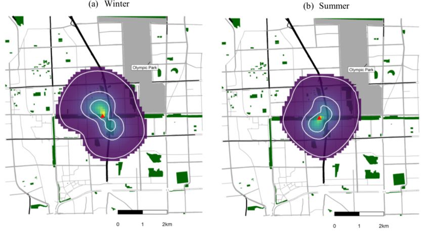
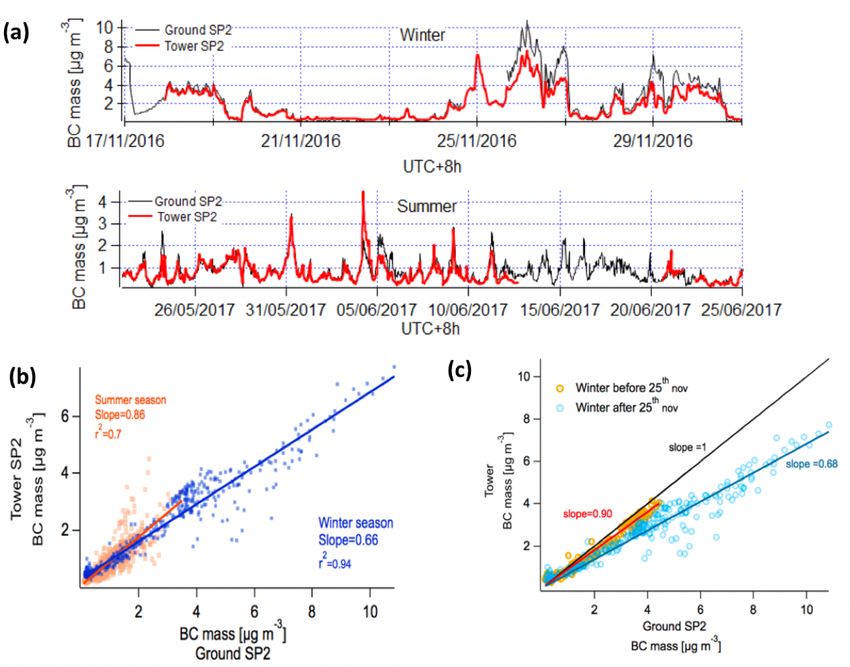
152                                             R. Joshi et al.: Direct measurements of black carbon fluxes in central Beijing

Figure 3. (a) Median of BC flux (black) and temperature (sensible heat) (yellow) co-spectrum multiplied by natural frequency (f ) and
normalised using total covariance against non-dimensional frequency. Data are binned into 44 logarithmically evenly spaced bins, and co-
spectra with total BC flux > 0 ng−2 s−1 and carefully selected frictional velocity for more turbulent periods (see Sect. 3.2) were chosen
for median averaging. A total of 223 (winter) and 170 (summer) cases are averaged. (b) Normalised cumulative co-spectra of BC flux and
sensible heat flux.

source characterisations. Firstly, here we compare the con-            an older generation of SP2 model but also possibly because
centrations of BC at both levels. Figure 4a shows the overlap          during the measurements the flux instrument operated at rel-
periods of both measurements, and Fig. 4b shows correla-               atively low laser power, either of which could have reduced
tion between the two sampling heights with an R 2 = 0.94               the signal-to-noise ratio of the scattering channels. There-
and 0.70 for winter and summer, respectively. During win-              fore, we have grouped our measurements into two groups:
ter, we observe a systematic difference between tower and              heavily coated particles(Esca > 3) and lightly coated parti-
ground measurement after the data gap on 25 November, cor-             cles (Esca < 3). The implication of heavily coated particles
responding to instrument maintenance for the ground-level              in this study refers to the combination of thickly coated and
SP2, which may have altered its performance. The differ-               moderately coated particles, while lightly coated particles in
ence was quantified by separating two periods and recal-               this study refer to the combination of small, thinly coated and
culating slopes comparing the tower and ground measure-                large, thinly coated particles, defined and grouped by Liu et
ments as shown in Fig. 4c. From this, we can infer that                al. (2019).
the ground measurements increased by 24 %. Furthermore,
for tower measurements, there were also particle line losses,          4.2   Black carbon fluxes
and the upper limit of line losses would be 34 %. This is
based on the highest difference observed in winter seasons             Figure 6 shows 30 min fluxes of BC mass and number for
between two levels, although the true losses are likely to             both the winter and summer periods. The signal-to-noise ra-
be lower than this, as we expect concentrations at ground              tio of the mass fluxes in particular is low, and fluxes vary
level to be higher. Secondly, we characterised the mixing              throughout the measuring period, due to the variability in
state of the particles for the tower level using the same scat-        emissions in the flux footprint, e.g. in response to activities
tering enhancement method as Liu et al. (2019), which is               and time of the day. However, mainly positive fluxes were
shown in Fig. 5. The two chosen scenarios include polluted             observed, confirming a net emission of BC from the city.
and clear periods to capture a variety of BC sources. Our              During the winter period, measurement coverage was lower
analysis shows similar characteristics of the physical prop-           (total number of 30 min averaging interval = 505) compared
erties of BC to those observed from the ground measure-                with the summer (total number of 30 min averaging in-
ments. Instead of four distinctive modes, we see some over-            terval = 976). Mean averaged mass fluxes (with associated
laps between those modes. This could be due to the use of              standard error) of 5.49 ± 0.49 and 6.10 ± 0.18 ng m−2 s−1

Atmos. Chem. Phys., 21, 147–162, 2021                                                      https://doi.org/10.5194/acp-21-147-2021
R. Joshi et al.: Direct measurements of black carbon fluxes in central Beijing                                                     153

Figure 4. (a) Comparisons of BC concentrations at 5 m (black) and 102 m (red) in winter and summer. (b) Correlation of BC concentrations
measured at the two different levels for winter (blue) and summer (orange). (c) Correlation of BC mass concentrations before and after
25 November.

                                                                       error (RE) of each averaging period following the method
                                                                       discussed by Finkelstein and Sims (2001). The mass flux is
                                                                       associated with a larger uncertainty than the number flux as
                                                                       the mass flux suffers from poor counting statistics since few
                                                                       particles with large BC mass make a large contribution to
                                                                       the total flux. The winter measurements are associated with
                                                                       higher uncertainty due to the lower atmospheric turbulence,
                                                                       and the higher incidence of extreme values is consistent with
                                                                       this noise. As such, no individual 30 min deposition events
Figure 5. BC particles physical properties on a clean and a polluted   can be discerned with any statistical certainty. Therefore, we
day. Scattering enhancement measured using the method discussed        did not unpick such events/criteria and instead discussed av-
by Liu et al. (2019). When the particle number density (colour) is     eraged flux results in this study. It is important to note that
> 70 % of the maxima in each panel, then the colour is set to red.     aerosol flux measurements tend to have higher RE than gas
                                                                       flux measurements. While the point-by-point data are of low
                                                                       precision, averaging of the fluxes according to either diurnal
were measured during the winter and summer, respectively.              cycle or wind sector can deliver more meaningful statistics,
For the BC number flux, averages of 261.25 ± 10.57 and                 and this is discussed in the following section. Additionally,
334.37 ± 0.37 cm−2 s−1 were measured. In order to remove               the summary of BC concentrations and fluxes is also pro-
any time-of-day biases associated with missing or filtered             vided in Table 1.
data, gaps in the data could be replaced with the corre-
sponding average diurnal value. This delivers modified BC              4.3   Local black carbon characterisation
mass fluxes of 5.22 and 6.06 ng m−2 s−1 for winter and
summer respectively and BC number fluxes of 252.41 and                 The flux footprint represents the local area that contributes
334.40 cm−2 s−1 . The uncertainty of the measurements is               to the measured flux. The shape and size of the flux foot-
shown with black error bars in Fig. 6. The calculation of              print is related to the sampling height, wind speed and direc-
such uncertainty was performed by calculating the random               tion, atmospheric stability, surface roughness, turbulence and

https://doi.org/10.5194/acp-21-147-2021                                                    Atmos. Chem. Phys., 21, 147–162, 2021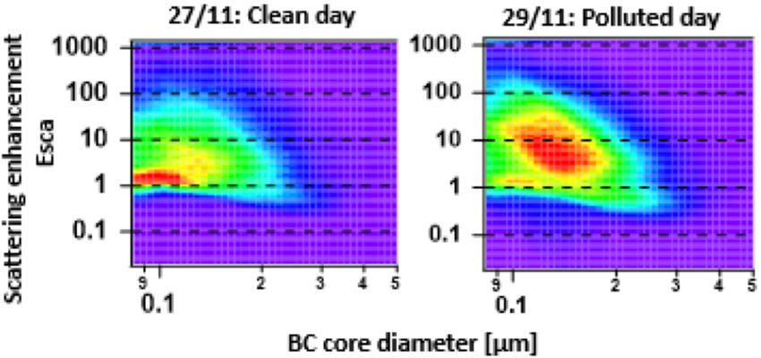
154                                            R. Joshi et al.: Direct measurements of black carbon fluxes in central Beijing

Figure 6. Time series of 30 min averaged fluxes during winter (blue) and summer (orange) for mass and number fluxes, with random errors
caused by associated uncertainties of the EC measurement system of this study (black bars).

the boundary layer height. Figure 7 depicts the extent of the         their spatial intensity according to their wind speed and di-
average flux footprint for the winter and summer measure-             rection in the following section.
ment periods, respectively. These footprints were generated
using the method presented by Squires et al. (2020), using the        4.4   Diurnal and wind sector trends
footprint model and theory discussed by Kljun et al. (2004)
and Metzger et al. (2012). However, the total numbers of in-          Figure 8 shows the diurnal cycles for mass and number
dividual footprints used to generate average campaign foot-           fluxes, for winter (blue) and summer (orange), and error
prints are slightly different to those presented by Squires et        bars represent the associated averaged random errors (e.g.
al. (2020), owing to slight differences in the respective in-         REhour ). These were calculated using the ensemble average
strument uptimes. The footprints were superimposed onto a             of RE for each diurnal hour as
map of Beijing at a grid resolution of 10 × 10 m. The ini-                         v
                                                                                   uN
tial comparison between the seasons shows that the averaged                      1u  X
                                                                      REhour = t         RE2 ,                               (4)
sizes of the footprints were similar. Here, the counter cir-                     N i=1 i
cles represent 30 %, 60 % and 90 % cumulative contribution
to the measured averaged fluxes from those regions. Dur-              where N is the number of 30 min averaging periods that en-
ing both seasons, the majority (up to 90 %) of contributions          tered into generating the average value for each hour of the
reached about 2 km from the IAP tower. However, within that           day.
range, maxima of the contribution occurred at a distance of              During winter, for both mass and number flux, there were
0.26 km. The major difference between the two seasons was             no clear diurnal cycles. In summer there was a clear peak at
the change in the dominant wind directions. During winter,            07:00, which could be related to traffic-related activities, but
the wind direction was predominantly from the north-west,             there was no distinctive peak for the evening rush hour. How-
and hence measurements are likely to have captured emis-              ever, the average flux values between the two seasons were
sions from Beitucheng West Road in the NW direction. Dur-             similar, which is consistent with the source being the same in
ing summer, winds were predominantly from the north-east              both seasons. For both seasons, BC diurnals showed similar
direction, capturing emissions from the major Jingzang Ex-            patterns to those of CO and NOx fluxes (Squires et al., 2020),
pressway. Since this analysis indicates the presence of traffic-      suggesting that traffic emissions are the dominant source of
related emissions, we have shown diurnal trends as well as            BC in this region of Beijing. Therefore, we additionally aver-

Atmos. Chem. Phys., 21, 147–162, 2021                                                    https://doi.org/10.5194/acp-21-147-2021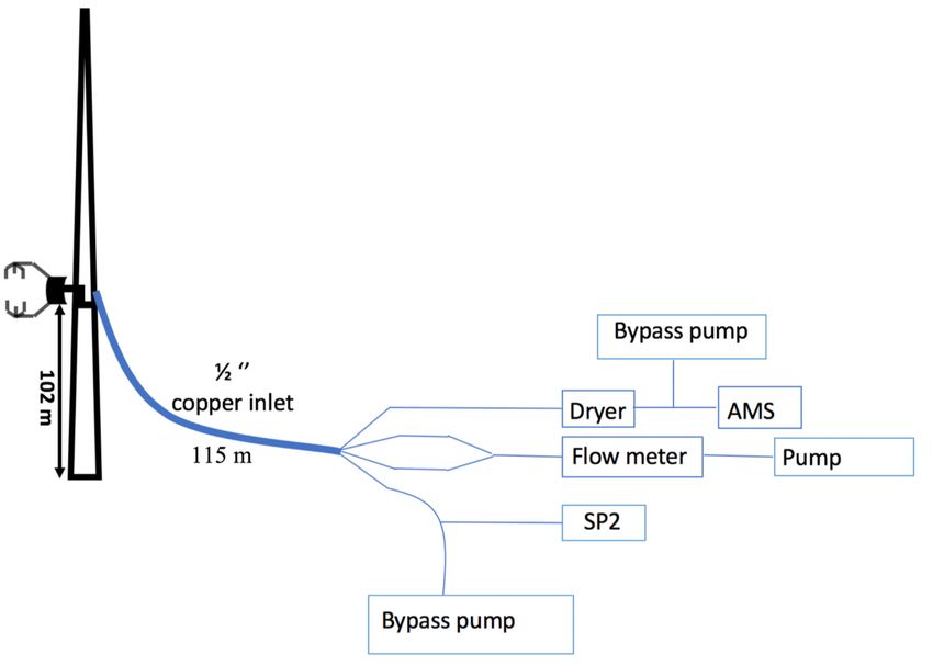
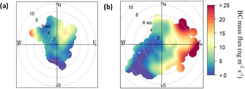
R. Joshi et al.: Direct measurements of black carbon fluxes in central Beijing                                                            155

Figure 7. Total average mass flux footprints for winter and summer seasons. The red spot on each plot is the location of the IAP tower, and
surrounding colours represent the magnitude of the intensity of the measured emission. The resolution of footprint is 100 m2 , the outermost
white line represents the 90 % cumulative spatial contribution of the total flux and the middle and the innermost lines represent 60 % and 30 %
contribution. Map was built using data from © OpenStreetMap contributors 2020. Distributed under a Creative Commons BY-SA License.
The ring roads are shown in black, and other roads are shown in grey. Parks/green spaces are shown in green.

Figure 8. Diurnal cycles for (a) number and (b) mass flux in summer and winter with error bars (standard errors, from the calculated
precision). For this analysis, storage-corrected fluxes are used to help understand ground-based emissions.

aged BC fluxes according to wind sector and generated polar               rection. The quantification of traffic emissions is discussed in
plots using OpenAir (Carslaw and Ropkins, 2012) for mass                  the following section.
fluxes, as shown in Fig. 9. This analysis clearly shows that
fluxes were largest in the NE direction during both seasons.              4.5   Flux for characterised black carbon particles
This is crucial as, during the winter, the NE is not a prominent
wind direction as we discussed in the footprint analysis sec-             In Sect. 4.1 the source apportionment of BC particles, ac-
tion. The analysis would suggest that the strongest sources               cording to their coating content, was discussed using the
lie in the NE and E directions, which is consistent with the              threshold value of Esca = 3; particles above this threshold
presence of a major traffic junction. During the summer, the              are defined as heavily coated, and the rest of the particles are
indications that the major source is traffic-related (such as the         lightly coated. The lightly coated mode contains BC particles
diurnal profile) are generally clearer, due to better coverage            with a strong association with traffic-related sources; how-
and signal-to-noise ratio, turbulence and favourable wind di-             ever within this mode, BC particles with Dc > 180 could pos-

https://doi.org/10.5194/acp-21-147-2021                                                        Atmos. Chem. Phys., 21, 147–162, 2021
156                                              R. Joshi et al.: Direct measurements of black carbon fluxes in central Beijing

Figure 9. BC mass flux distribution by wind direction and wind speed for the (a) winter and (b) summer analysis done using OpenAir
software (Carslaw and Ropkins, 2012).

Table 1. Concentration and flux statistics of BC measurements at     Table 2. Winter season percentage values of concentrations and
the IAP tower. The 5 Hz concentration measurements were resam-       fluxes for coating classification and size classification. For coating
pled 30 min before performing statistical calculations.              classification, the total particles were separated according to coat-
                                                                     ing contents using the threshold of Esca = 3 for both BC mass and
  Concentrations           BC mass               BC number           number. For size classification, the total particles were separated at
                           (µg m−3 )              (cm−3 )            Dc = 180 nm, for BC mass and number. During summer, such an
                                                                     analysis was not performed due to limitations of the instrument at
                       Winter   Summer         Winter   Summer       the time of the experiment.
  Mean                   1.90          0.70    677.70    330.00
  Median                 1.32          0.53    495.92    268.57                                             Concentrations     Fluxes
  Standard deviation     1.54          0.51    558.33    239.90                                                        (%)        (%)
  Percentile                                                                                                  Coating classification
  5th                    0.37          0.14    126.85     77.77          BC mass         Heavily coated                23.2        7.7
  95th                   4.70          1.56   1656.40    751.70                          Lightly coated                76.8       92.3
  Number of               716          1428      716       1428          BC Number       Heavily coated                18.8        7.7
  observations                                                                           Lightly coated                81.2       92.3
  Fluxes                   BC mass               BC number
                                                                                                                Size classification
                         (ng m−2 s−1 )           (cm−2 s−1 )
                                                                         BC mass         Dc > 180 nm                   63.8       58.3
                       Winter   Summer         Winter   Summer
                                                                                         Dc < 180 nm                   36.2       41.7
  Mean                   5.49          6.10    261.25    334.37
  Median                 4.13          3.58    203.71    229.01          BC number       Dc > 180 nm                   15.6        7.5
  Standard deviation    14.65          9.07    439.50    376.85                          Dc < 180 nm                   84.4       92.5

  Percentile
  5th                  −13.87     −3.45        218.77   −43.66       most a quarter of the BC mass concentrations (and slightly
  95th                  29.13     22.78       1040.04   1091.60
                                                                     less than a quarter if we consider number concentrations)
  Number of               505          976       505           976   measured at IAP were from the heavily coated mode, and
  observations                                                       the rest of the particles were from the lightly coated mode. In
                                                                     order to quantify what proportion of these particles was emit-
                                                                     ted locally, fluxes of each individual categories were also cal-
                                                                     culated, and their average values are also summarised in Ta-
sibly be associated with solid fuel burning, according to BC         ble 2. We can see that the contribution of BC particles emitted
source apportionment, discussed by Liu et al. (2019). There-         from heavily coated was smaller than 8 % for both BC mass
fore, in this analysis, we firstly separated BC mass and BC          and number fluxes, with the lightly coated mode accounting
number concentrations using a threshold value of Esca = 3            for 92.3 % of both fluxes.
and defined this characteristic as coating classification. Ad-          Regarding size classification, it is important to note that
ditionally, we used a threshold of Dc = 180 nm to perform            there were fewer particles above this range; yet they con-
the size classification.                                             tributed significantly to the concentration in mass space.
   The average mass and number concentration of lightly              Therefore, this analysis suffers from poor counting statistics,
coated and heavily coated particles are shown in Table 2. Al-        and we cannot reliably quantify emissions for particles with

Atmos. Chem. Phys., 21, 147–162, 2021                                                     https://doi.org/10.5194/acp-21-147-2021
R. Joshi et al.: Direct measurements of black carbon fluxes in central Beijing 157
Dc > 180 nm. However, the general trend for both BC mass Table 3. Estimated ratios of BC / NOx and BC / CO for gaso-
and BC number quantity in Table 2 for the size classification line engines and diesel engines. An overview of on-road vehicu-
shows that the average fraction of particles Dc > 180 nm is lar emissions and their control in China by Wu et al. (2017) sum-
higher for concentrations compared to their fraction of the marised NOx , CO and PM2.5 emission regulation targets in China.
total flux measurements, indicating that the majority of these The BC / PM2.5 fractions for gasoline were taken from European
guideline of emissions controls, as such fractions are not available
particles are from outside of the flux footprint. As the ma-
for China. Since PM2.5 controls for LDGVs were only introduced
jority of emissions within the flux footprints are in the form recently within China 5 controls, our estimates could not be per-
of lightly coated particles, this is consistent with this particle formed according to previous standards. Observed values corre-
type being associated with traffic-related activities. spond to ratios shown in Fig. 10. Dates are given in yyyy/mm/d.
TBD denotes standards that are “to be decided”.
5 Discussion Implementation BC / NOx BC / CO
date
5.1 Comparison with NOx and CO emissions Gasoline emissions standards
With the assumption that CO and NOx are co-emitted with China 1 2000/7/1 – –
BC by combustion sources, we have investigated the corre- China 2 2005/7/1 – –
China 3 2008/7/1 – –
lations of their measured fluxes with BC using orthogonal
China 4 2011/7/1 – –
distance regression. These are shown in Fig. 10a and b, for
China 5 2017/1/1 0.009 0.00054
CO and NOx , respectively, and the gradients in each plot cor- China 6a TBD 0.009 0.00108
respond to the emission flux ratios. The comparison with CO China 6b TBD 0.01031 0.0007
fluxes shows BC / CO mass ratios of 0.0007 and 0.0011 for
winter and summer, respectively. During the summer, this ra- Diesel emission standards
tio is 37 % larger than in winter. Our study has shown similar China I 2001/9/1 0.026 0.046
emissions of total averaged BC in the two seasons; however, China II 2004/9/1 0.012 0.021
this is not the case for CO. During winter, cold-start con- China III 2008/1/1 0.012/0.018 0.027/0.017
ditions may explain the increase in CO emission, which is China IV 2015/1/1 0.0032/0.005 0.008/0.004
further discussed by Squires et al. (2020). The comparison China V 2017/1/1 0.0057/0.009 0.008/0.004
with NOx fluxes shows BC / NOx ratios are the same be- Observed Winter 0.0058 0.0007
tween seasons, 0.0058 and 0.0052 for winter and summer, values Summer 0.0052 0.0011
respectively. The relationship in winter shows more scatter
due to a poor signal-to-noise ratio. Nevertheless, the consis-
tency of the NOx slopes is highly encouraging as the iden- cently from 1 January 2017 as part of China 5 controls. If we
tical relationship is not only consistent with the emissions compare our measured emission ratios as shown in Fig. 10
being from a singular dominant source, i.e. vehicles, but also with the values in Table 3, we find that the measured val-
provides confidence in the measurements, given that a phys- ues are in a similar range as the ratio of China 5 limit levels
ically different instrument was used in the two seasons. for gasoline emissions, noting that diesel vehicles are banned
Following a similar vehicular European regulation sys- from central Beijing during the daytime and are therefore not
tem for emission controls, China has started to adopt emis- expected to contribute. Making the implicit assumption that
sion regulation targets. The limits imposed cover the major the legal limits are a fair reflection of actual emissions, this
pollutants CO, NOx , non-methane hydrocarbon (NMHC), is in a good agreement.
HC + NOx and PM (which refers to PM2.5 ) for both light-
duty gasoline vehicles (LDGVs) and heavy-duty diesel en- 5.2 Emission inventory
gines (HDDEs), as summarised by Wu et al. (2017). How-
ever, to the best of our knowledge, reliable values of BC Here we compare our measurements with the Multi-
fraction within PM2.5 are not available in literature for resolution Emission Inventory for China (MEIC; available at
China’s regulation standards. Therefore, we used the aver- http://www.meicmodel.org/, last access: 2 November 2019),
age BC / PM2.5 ratios for gasoline engines from the Euro- developed at Tsinghua University (e.g Zhang et al., 2015).
pean guidelines of emissions controls as stated in Table 3.2.1 The inventory uses spatial proxies (e.g. population and en-
of Ntziachristos and Samaras (2017), which are 0.12 and ergy consumption statistics) to downscale emissions from a
0.57 for gasoline and diesel engines, respectively. Using national and provincial scale to finer resolution (Biggart et
these ratios, we have estimated BC / NOx and BC / CO ra- al., 2020; Qi et al., 2017). In this study, BC emissions for the
tios implied with each of China emission’s standards for both year 2013 at a resolution of 3 × 3 km were used, which was
LDGVs and HDDEs, as shown in Table 3. It is important to the most recent version available at the time of this study.
note that PM2.5 controls for LDGVs were only introduced re- The inventory emission values were extracted for the area
https://doi.org/10.5194/acp-21-147-2021 Atmos. Chem. Phys., 21, 147–162, 2021158 R. Joshi et al.: Direct measurements of black carbon fluxes in central Beijing
Figure 10. BC mass flux with (a) NOx flux (Squires et al., 2020) and (b) CO flux (Squires et al., 2020) for winter and summer with calculated
BC / NOx and BC / CO ratios and NOx and CO fluxes converted to the same units as our measurements.
covered by the averaged flux footprint (see Sect. 4.3) follow- noted that the emissions of NOx and CO from the inventory
ing the same approach as Squires et al. (2020). are also high compared with measured fluxes, as reported by
Figure 11 shows a comparison of the diurnal cycles be- Squires et al. (2020). The overestimation of emissions in this
tween measured fluxes and the MEIC 2013 emission inven- region may reflect the limited suitability of the proxies used
tory for (a) winter and (b) summer, where the diurnal cycles in downscaling the emissions from a regional, provincial res-
for each sector (transport, industry, agriculture, residential olution to the 3 km scale used here, as noted by Zheng et
and power) were generated from the MEIC 2013 estimates. al. (2017). However, the overestimation of the ratios high-
The inventory has a broadly similar temporal pattern to lights that it is likely that BC emissions are overestimated
the observed fluxes but overestimates the total BC emissions in MEIC, at least for the region considered here. The diur-
from the flux footprint by a factor of 59 and 47 during the nal patterns of emissions, in contrast, are in relatively good
winter and summer periods, respectively. Since the transport agreement.
sector contributes 63 % and 80 % of the overall BC emissions
in the MEIC inventory, the average emissions of the transport
sector in isolation were also compared with the measured 6 Conclusion
flux. This reduced the discrepancy to within a factor of 38
for both winter and summer periods. Local emissions of BC fluxes were measured using the
The reduction in emissions in Beijing from 2013 to 2017 eddy covariance method in Beijing as part of the APHH
has been analysed by Cheng et al. (2019) using the MEIC project during the winter of 2016 and summer of 2017
model in combination with a local bottom-up emission in- from the IAP tower, the first application of this ap-
ventory. This study concludes that the reduction in PM2.5 proach to an urban environment. During both seasons,
emissions from the transport sector is negligible, as since average BC mass flux and number fluxes remained sta-
2013 there has been an increase in stringent traffic manage- ble. In the case of BC mass fluxes, average values of
ment and fuel control policies, but vehicle densities have in- 5.5 ± 0.49 and 6.1 ± 0.18 ng m−2 s−1 were measured during
creased, keeping emissions from the transport sector steady. the winter and summer seasons, respectively. In the case
This is also discussed on a national level for BC emissions of BC number fluxes, average values of 261.3 ± 10.57 and
from the transport sector by Zheng et al. (2018), and it was 334.4 ± 0.37 cm−2 s−1 were measured for the winter and
concluded that emissions from the transport sectors remained summer seasons, respectively. The similarity in the magni-
steady between 2010 and 2017. Therefore, such a large dis- tude of emissions between seasons suggests that there was
crepancy is unlikely to be due to changes in actual emissions no major additional source in winter associated with heat-
between 2013 and 2017. We also compared BC / CO and ing, consistent with the use of district heating in central Bei-
BC / NOx ratios for the transport emission data in MEIC, jing. Flux footprints (up to 2 km from the IAP tower in both
which were 0.0066, 0.0423 and 0.0072, 0.0425 for the winter seasons) and wind sector-based analysis showed emission
and summer seasons, respectively. Compared to the observed sources are strongest to the NE and E of the IAP tower, where
ratios, these are factors of 9.4 and 6.5 too high for the ratios a major road is situated, confirming the presence of traffic
with CO in winter and summer respectively and 7.3 and 8.1 emissions. The contribution of traffic emission was quanti-
for the ratios with NOx . This implies that the BC emissions fied by classifying total BC particles according to coating
from traffic are overestimated in MEIC, although it should be thickness during the winter season, following the previous
observation that traffic emits smaller, more lightly coated
Atmos. Chem. Phys., 21, 147–162, 2021 https://doi.org/10.5194/acp-21-147-2021R. Joshi et al.: Direct measurements of black carbon fluxes in central Beijing 159
Figure 11. Comparison between measured emissions and the MEIC 2013 emission inventory for (a) winter and (b) summer for the flux
footprint area (Sect. 4.3). Diurnal variation from the MEIC estimates is used for the diurnal cycles for emissions of all sectors (sum of
emissions from transport, industry, residential and power) and the transport sector in isolation.
particles. The analysis indicated traffic emissions were ap- Author contributions. RJ made the measurements, performed data
proximately 92 % of the total measured flux for both BC analysis and wrote the paper with support from JA, HC and DL. DL
mass and BC number fluxes, and the rest was possibly as- helped with developing the toolkit for the preprocessing of SP2 flux
sociated with solid fuel burning. In terms of the overall con- data and provided guidance with source apportionment of work.
centrations, the heavily coated particles represented 23 % and NM installed and maintained the tower EC measurement setup. EN
and BL helped RJ with flux calculations and the use of the EddyPro
19 % of the BC mass and number concentrations respec-
software. FS and JL provided flux footprint calculations, with cor-
tively. The higher presence of the heavily coated particles responding emission inventory data. YW, XP and PF allowed the
in concentration measurements but not local fluxes suggests use of their SP2 instrument during the summer season. SK and SG
advection of a source outside the footprint and is indicative provided the mixed layer height data. QZ and RW provided MEIC
of regional pollution. The measurements were also compared inventory data, and OW helped with the interpretation of the inven-
with NOx and CO fluxes and the corresponding emission ra- tory values. MF provided technical support for maintenance of the
tios BC / CO and BC / NOx were inferred. The BC / NOx SP2 instruments. HC and JA are PhD supervisors of RJ. All the au-
ratio was found to be consistent between seasons, and both thors read and improved the paper.
ratios were in general agreement with ratios implied by the
China emission standards. Finally, the measured emissions
were compared with the MEIC 2013 inventory. The magni- Competing interests. The authors declare that they have no conflict
tude of the transport sector emissions in the inventory alone of interest.
was significantly larger (by over an order of magnitude) than
our measurements. Such a discrepancy cannot solely be ex-
plained by changes in emissions since 2013, indicating that Special issue statement. This article is part of the special issue
“In-depth study of air pollution sources and processes within Bei-
there are other inaccuracies, likely in the proxies used to
jing and its surrounding region (APHH-Beijing) (ACP/AMT inter-
downscale the emissions to an urban landscape as noted by journal SI)”. It is not associated with a conference.
Zheng et al. (2017). The shape of the diurnal variation in the
inventory was in better agreement; however, the BC / CO and
BC / NOx ratios from the MEIC inventory were substantially Acknowledgements. Rutambhara Joshi’s PhD was supported by the
larger than the measured ratios, which could indicate that an National Centre of Atmospheric Science (NCAS). The field mea-
inaccuracy in the assumed BC emission profile is at least par- surements were supported by the Newton Fund, administered by
tially responsible for the disagreement. This indicates that the UK Natural Environment Research Council (NERC) through
BC emissions in the inventory are overestimated, at least in the AIR-POLL and AIRPRO projects of the Air Pollution and Hu-
the urban area of Beijing. man Health in a Chinese Megacity (APHH-Beijing) programme.
Data availability. Processed data are available in the APHH- Financial support. This research has been supported by the
Beijing project database in the Centre for Environmental Data Anal- Natural Environment Research Council (grant nos. NE/N006992/1,
ysis Archive (http://data.ceda.ac.uk/badc/aphh/data/beijing/, Flem- NE/N006976/1, NE/N006917/1, NE/N007123/1 and
ing et al., 2017). Raw data are available on request. NE/N00700X/1).
https://doi.org/10.5194/acp-21-147-2021 Atmos. Chem. Phys., 21, 147–162, 2021160 R. Joshi et al.: Direct measurements of black carbon fluxes in central Beijing
Review statement. This paper was edited by Markus Petters and re- Finkelstein, P. L. and Sims, P. F.: Sampling error in eddy correlation
viewed by two anonymous referees. flux measurements, J. Geophys. Res.-Atmos., 106, 3503–3509,
2001.
Fleming, Z. L., Lee, J. D., Liu, D., Acton, J., Huang, Z., Wang, X.,
Hewitt, N., Crilley, L., Kramer, L., Slater, E., Whalley, L., Ye, C.,
References and Ingham, T.: APHH: Atmospheric measurements and model
results for the Atmospheric Pollution & Human Health in a Chi-
Barr, A. G., Richardson, A. D., Hollinger, D. Y., Papale, D., nese Megacity, Centre for Environmental Data Analysis Archive,
Arain, M. A., Black, T. A., Bohrer, G., Dragoni, D., Fischer, available at: http://data.ceda.ac.uk/badc/aphh/data/beijing/ (last
M. L., Gu, L., Law, B. E., Margolis, H. A., Mccaughey, J. access: 4 January 2021), 2017.
H., Munger, J. W., Oechel, W., and Schaeffer, K.: Use of Foken, T. and Wichura, B.: Tools for quality assessment of surface-
change-point detection for friction-velocity threshold evaluation based flux measurements, Agr. Forest Meteorol., 78, 83–105,
in eddy-covariance studies, Agr. Forest Meteorol., 171–172, 31– https://doi.org/10.1016/0168-1923(95)02248-1, 1996.
45, https://doi.org/10.1016/j.agrformet.2012.11.023, 2013. Gao, R. S., Schwarz, J. P., Kelly, K. K., Fahey, D. W., Watts, L.
Barrington-Leigh, C., Baumgartner, J., Carter, E., Robinson, B. E., A., Thompson, T. L., Spackman, J. R., Slowik, J. G., Cross, E.
Tao, S., and Zhang, Y.: An evaluation of air quality, home heating S., Han, J. H., Davidovits, P., Onasch, T. B., and Worsnop, D.
and well-being under Beijing’s programme to eliminate house- R: A novel method for estimating light-scattering properties of
hold coal use, 4, 416–423, https://doi.org/10.1038/s41560-019- soot aerosols using a modified single-particle soot photometer,
0386-2, 2019. Aerosol Sci. Tech., 41, 125–135, 2007.
Biggart, M., Stocker, J., Doherty, R. M., Wild, O., Hollaway, Harrison, R. M., Deacon, A. R., Jones, M. R., and Appleby, R.
M., Carruthers, D., Li, J., Zhang, Q., Wu, R., Kotthaus, S., S.: Sources and processes affection concentrations of PM10
Grimmond, S., Squires, F. A., Lee, J., and Shi, Z.: Street- and PM2.5 particulate matter in Birmingham (U.K.), At-
scale air quality modelling for Beijing during a winter 2016 mos. Environ., 31, 4103–4117, https://doi.org/10.1016/S1352-
measurement campaign, Atmos. Chem. Phys., 20, 2755–2780, 2310(97)00296-3, 1997.
https://doi.org/10.5194/acp-20-2755-2020, 2020. Hodnebrog, Ø., Myhre, G., and Samset, B. H.: How shorter black
Bond, T. C. and Bergstrom, R. W.: Light Absorption by Carbona- carbon lifetime alters its climate effect, Nat. Commun., 5, 1–7,
ceous Particles: An Investigative Review, Aerosol Sci. Tech., 40, 2014.
27–67, https://doi.org/10.1080/02786820500421521, 2006. Järvi, L., Nordbo, A., Rannik, Ü., Haapanala, S., Mammarella,
Bond, T. C., Streets, D. G., Yarber, K. F., Nelson, S. I., Pihlatie, M., Vesala, T., and Riikonen, A.: Urban nitrous-
M., Woo, J.-H., and Klimont, Z.: A technology-based oxide fluxes measured using the eddy-covariance technique in
global inventory of black and organic carbon emissions Helsinki, Finland, Boreal Environ. Res., 19, 108–121, 2014.
from combustion, J. Geophys. Res.-Atmos., 109, D14203, Jassen, N. A. H., Gerlofs-Nijland, M. E., Lanki, T., Salo-
https://doi.org/10.1029/2003JD003697, 2004. nen, R. O., Cassee, F., Hoek, G., Fischer, P., Brunekreef,
Bond, T. C., Doherty, S. J., Fahey, D. W., Forster, P. M., Berntsen, B., and Krzyzonowsk, M.: Health Effects of Black Car-
T., Deangelo, B. J., Flanner, M. G., Ghan, S., K??rcher, B., bon, World Health Organization, Regional Office for Eu-
Koch, D., Kinne, S., Kondo, Y., Quinn, P. K., Sarofim, M. C., rope, available at: http://www.euro.who.int/__data/assets/pdf_
Schultz, M. G., Schulz, M., Venkataraman, C., Zhang, H., Zhang, file/0004/162535/e96541.pdf (last access: 5 January 2021),
S., Bellouin, N., Guttikunda, S. K., Hopke, P. K., Jacobson, M. 2012.
Z., Kaiser, J. W., Klimont, Z., Lohmann, U., Schwarz, J. P., Kaimal, J. C. and Finnigan, J. J.: Atmospheric boundary layer flows:
Shindell, D., Storelvmo, T., Warren, S. G., and Zender, C. S.: their structure and measurement, Oxford university press, New
Bounding the role of black carbon in the climate system: A sci- York, USA, 1994.
entific assessment, J. Geophys. Res.-Atmos., 118, 5380–5552, Kaimal, J. C., Wyngaard, J., Izumi, Y., and Cote, O.: Spectral char-
https://doi.org/10.1002/jgrd.50171, 2013. acteristics of surface-layer turbulence, Q. J. Roy. Meteor. Soc.,
Cao, G., Zhang, X., and Zheng, F.: Inventory of black carbon and or- 98, 563–589, https://doi.org/10.1256/smsqj.41706, 1972.
ganic carbon emissions from China, Atmos. Environ., 40, 6516– Kljun, N., Calanca, P., Rotach, M. W., and Schmid,
6527, https://doi.org/10.1016/j.atmosenv.2006.05.070, 2006. H. P.: A simple parameterisation for flux footprint
Carslaw, D. C. and Ropkins, K.: Openair – An r package for air predictions, Bound.-Lay. Meteorol., 112, 503–523,
quality data analysis, Environ. Model. Softw., 27–28, 52–61, https://doi.org/10.1023/B:BOUN.0000030653.71031.96, 2004.
https://doi.org/10.1016/j.envsoft.2011.09.008, 2012. Kotthaus, S. and Grimmond, C. S. B.: Identification of
Cheng, J., Su, J., Cui, T., Li, X., Dong, X., Sun, F., Yang, Y., Micro-scale Anthropogenic CO2 , heat and moisture
Tong, D., Zheng, Y., Li, Y., Li, J., Zhang, Q., and He, K.: sources – Processing eddy covariance fluxes for a dense
Dominant role of emission reduction in PM2.5 air quality im- urban environment, Atmos. Environ., 57, 301–316,
provement in Beijing during 2013–2017: a model-based de- https://doi.org/10.1016/j.atmosenv.2012.04.024, 2012.
composition analysis, Atmos. Chem. Phys., 19, 6125–6146, Kotthaus, S. and Grimmond, C. S. B.: Energy exchange in a
https://doi.org/10.5194/acp-19-6125-2019, 2019. dense urban environment – Part I: Temporal variability of long-
Emerson, E. W., Katich, J. M., Schwarz, J. P., McMeek- term observations in central London, Urban Clim., 10, 261–280,
ing, G. R., and Farmer, D. K.: Direct Measurements https://doi.org/10.1016/j.uclim.2013.10.002, 2014.
of Dry and Wet Deposition of Black Carbon Over a Kotthaus, S. and Grimmond, C. S. B.: Atmospheric boundary-layer
Grassland, J. Geophys. Res.-Atmos., 123, 12,277-12,290, characteristics from ceilometer measurements. Part 1: A new
https://doi.org/10.1029/2018JD028954, 2018.
Atmos. Chem. Phys., 21, 147–162, 2021 https://doi.org/10.5194/acp-21-147-2021You can also read


