Identifying areas prone to coastal hypoxia - the role of topography - Biogeosciences
←
→
Page content transcription
If your browser does not render page correctly, please read the page content below
Biogeosciences, 16, 3183–3195, 2019
https://doi.org/10.5194/bg-16-3183-2019
© Author(s) 2019. This work is distributed under
the Creative Commons Attribution 4.0 License.

Identifying areas prone to coastal hypoxia – the role of topography
Elina A. Virtanen1,2 , Alf Norkko3,4 , Antonia Nyström Sandman5 , and Markku Viitasalo1
1 Marine  Research Centre, Finnish Environment Institute, Helsinki, 00790, Finland
2 Department  of Geosciences and Geography, University of Helsinki, Helsinki, 00014, Finland
3 Tvärminne Zoological Station, University of Helsinki, Hanko, 10900, Finland
4 Baltic Sea Centre, Stockholm University, Stockholm, 10691, Sweden
5 AquaBiota Water Research, Stockholm, 11550, Sweden

Correspondence: Elina A. Virtanen (elina.a.virtanen@environment.fi)

Received: 10 April 2019 – Discussion started: 16 April 2019
Revised: 25 June 2019 – Accepted: 30 July 2019 – Published: 27 August 2019

Abstract. Hypoxia is an increasing problem in marine              fluence coastal oxygen dynamics. Developed models could
ecosystems around the world. While major advances have            boost the performance of biogeochemical models, aid devel-
been made in our understanding of the drivers of hypoxia,         oping nutrient abatement measures and pinpoint areas where
challenges remain in describing oxygen dynamics in coastal        management actions are most urgently needed.
regions. The complexity of many coastal areas and lack of
detailed in situ data have hindered the development of mod-
els describing oxygen dynamics at a sufficient spatial res-
olution for efficient management actions to take place. It        1   Introduction
is well known that the enclosed nature of seafloors and re-
duced water mixing facilitates hypoxia formation, but the         Hypoxia is a key stressor of marine environments, occurring
degree to which topography contributes to hypoxia forma-          in over 400 physically diverse marine ecosystems worldwide
tion and small-scale variability of coastal hypoxia has not       (Diaz and Rosenberg, 1995b, 2008; Conley et al., 2009). De-
been previously quantified. We developed simple proxies           clining oxygen levels have been recorded in fjords, estuaries,
of seafloor heterogeneity and modeled oxygen deficiency in        and in coastal and open-sea areas, such as the Chesapeake
complex coastal areas in the northern Baltic Sea. Accord-         Bay, Gulf of Mexico, Japan Sea, Baltic Sea and the Black
ing to our models, topographical parameters alone explained       Sea (Gilbert et al., 2010; Carstensen et al., 2014). It is clear
 ∼ 80 % of hypoxia occurrences. The models also revealed          that our oceans are losing their breath, and recent projections
that less than 25 % of the studied seascapes were prone to        indicate that anoxic zones devoid of higher life will be in-
hypoxia during late summer (August–September). However,           creasing in the forthcoming decades (Frölicher et al., 2009;
large variation existed in the spatial and temporal patterns of   Meier et al., 2011a, 2012a), with severe consequences for
hypoxia, as certain areas were prone to occasional severe hy-     marine ecosystems (Breitburg et al., 2018).
poxia (O2 < 2 mg L−1 ), while others were more susceptible to        The lack of oxygen alters the structure and functioning of
recurrent moderate hypoxia (O2 < 4.6 mg L−1 ). Areas identi-      benthic communities (Nilsson and Rosenberg, 2000; Gray
fied as problematic in our study were characterized by low        et al., 2002; Karlson et al., 2002; Valanko et al., 2015),
exposure to wave forcing, high topographic shelter from sur-      disrupts bioturbation activities (Timmermann et al., 2012;
rounding areas and isolation from the open sea, all contribut-    Villnas et al., 2012, 2013; Norkko et al., 2015), changes
ing to longer water residence times in seabed depressions.        predator–prey relationships (Eriksson et al., 2005) and may
Deviations from this topographical background are probably        lead to mass mortalities of benthic animals (Vaquer-Sunyer
caused by strong currents or high nutrient loading, thus im-      and Duarte, 2008). Hypoxia does not only affect organisms
proving or worsening oxygen status, respectively. In some         of the seafloor, but also influences biogeochemical cycling
areas, connectivity with adjacent deeper basins may also in-      and benthic–pelagic coupling (Gammal et al., 2017). Hy-
                                                                  poxia can increase releases of nutrients from the sediment

Published by Copernicus Publications on behalf of the European Geosciences Union.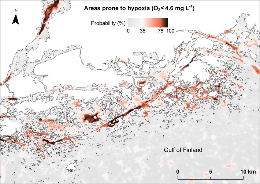
3184                                                           E. A. Virtanen et al.: Identifying areas prone to coastal hypoxia

and thus promote planktonic primary production and sedi-             mine the degree to which seascape structure restricting wa-
mentation, which in turn leads to enhanced microbial con-            ter movement contributes to hypoxia formation has not been
sumption of oxygen (Conley et al., 2002; Kemp et al., 2009;          quantified. Analytical and theoretical frameworks developed
Middelburg and Levin, 2009). This creates a self-sustaining          specifically for terrestrial environments, such as landscape
process, often referred to as the “vicious circle of eutrophi-       heterogeneity or patchiness, are analogous in marine envi-
cation” (Vahtera et al., 2007), which may hamper the effects         ronments and are equally useful for evaluating links between
of nutrient abatement measures.                                      ecological functions and spatial patterns in a marine context.
   Biogeochemical processes contributing to hypoxia forma-           We tested how a large fraction of hypoxia occurrences could
tion are well known. Factors affecting the development of hy-        be explained only by the structural complexity of seascapes,
poxia are usually associated with the production of organic          without knowledge on hydrographical or biogeochemical pa-
matter, level of microbial activity and physical conditions          rameters. We adopted techniques and metrics from landscape
creating stratification and limited exchange or mixing of wa-        ecology and transferred them to the marine environment, and
ter masses (Conley et al., 2009, 2011; Rabalais et al., 2010;        we (1) examined if spatial patterns in seascapes can explain
Fennel and Testa, 2019). Coastal hypoxia is common in areas          the distribution of hypoxia, (2) defined the relative contribu-
with moderate or high anthropogenic nutrient loading, high           tion of seascape structure to hypoxia formation and (3) es-
primary productivity and complex seabed topography limit-            timated the potential ranges of hypoxic seafloors in coastal
ing lateral movement of the water. Shallow-water hypoxia is          areas. To achieve this, we concentrated on extremely het-
often seasonal. It is associated with warming water tempera-         erogeneous and complex archipelago areas in the northern
tures and enhanced microbial processes and oxygen demand             Baltic Sea, where coastal hypoxia is a common and an in-
(Buzzelli et al., 2002; Conley et al., 2011; Caballero-Alfonso       creasing problem (Conley et al., 2011; Caballero-Alfonso et
et al., 2015; van Helmond et al., 2017).                             al., 2015).
   Projecting patterns and spatial and temporal variability of
hypoxia is necessary for developing effective management
actions. Thus three-dimensional coupled hydrodynamic–                2     Data and methods
biogeochemical models have been created for several sea ar-
eas around the world, such as the Gulf of Mexico (Fennel et          2.1    Study area
al., 2011, 2016), Chesapeake Bay (Scully, 2013, 2016; Testa
et al., 2014), the North Sea (Hordoir, 2018) and the Baltic          The studied area covers the central northern Baltic Sea
Sea (Eilola et al., 2009, 2011; Meier et al., 2011a, 2012a, b).      coastal rim, 23 500 km2 of Finnish territorial waters from the
These models simulate various oceanographic, biogeochem-             Bothnian Bay to the eastern Gulf of Finland and 5100 km2
ical, and biological processes using atmospheric and climatic        of Swedish territorial waters in the Stockholm archipelago in
forcing and information on nutrient loading from rivers.             the Baltic Proper. Oxygen dynamics in the deeper areas of
While such models are useful for studying processes at the           the Gulf of Finland and Stockholm archipelago are strongly
scale of kilometers, and aid in defining hypoxia abatement           affected by oceanography and biogeochemistry of the central
at the basin scale, their horizontal resolution is too coarse        Baltic Proper, not reflecting the dynamics of coastal hypoxia
(often 1–2 nmi, nautical miles) for accurately describing pro-       (Laine et al., 1997), and were therefore excluded from this
cesses in coastal areas. Lack of detailed data on water depth,       study. The outer archipelago of Finland is relatively exposed
currents, nutrient loads, stratification and local distribution of   with various sediment and bottom habitat types, while the
freshwater discharges (Breitburg et al., 2018) (not to mention       inner archipelago is more complex and shallower, but main-
computational limitations) usually prevents the application          tains a higher diversity of benthic habitats and sediment types
of biogeochemical models developed to large geographical             (Valanko et al., 2015). The inner archipelago of Stockholm
areas at finer horizontal resolutions (< 100 m). Understand-         is an equally complex archipelago area, with a large number
ing spatial variability of hypoxia in topographically complex        of islands, straits and coves. Freshwater outflow from Lake
coastal environments has therefore been impeded by the lack          Mälaren creates an estuarine environment where freshwater
of useful methods and systematic, good-quality data (Diaz            meets the more saline water in the Baltic Proper.
and Rosenberg, 2008; Rabalais et al., 2010; Stramma et al.,             In order to evaluate differences in oxygen deficiency be-
2012). Finding alternative ways to pinpoint areas prone to           tween coastal areas, the study area was divided into five
coastal hypoxia could facilitate the management and deter-           regions as defined by the EU Water Framework Directive
mination of efficient local eutrophication abatement mea-            (2000/60/EC) (WFD, 2000): the Archipelago Sea (AS), the
sures.                                                               eastern Gulf of Finland (EGoF), the Gulf of Bothnia (GoB),
   It is widely recognized that the semienclosed nature of the       the Stockholm archipelago (SA) and the western Gulf of Fin-
seafloors, and associated limited water exchange, is a sig-          land (WGoF) (Fig. 1). Small skerries and sheltered bays char-
nificant factor in the formation of hypoxia in coastal wa-           acterize AS, EGoF and WGoF, whereas the narrower band of
ters (Diaz and Rosenberg, 1995a; Virtasalo et al., 2005; Ra-         islands forms relatively exposed shores in GoB. Deep, elon-
balais et al., 2010; Conley et al., 2011). However, to deter-        gated channels of bedrock fractures can reach depths of over

Biogeosciences, 16, 3183–3195, 2019                                                      www.biogeosciences.net/16/3183/2019/
E. A. Virtanen et al.: Identifying areas prone to coastal hypoxia                                                                3185

                                                                      toms of the lack of oxygen, and this limit has been commonly
                                                                      used in various global reviews (Diaz and Rosenberg, 1995b,
                                                                      2008). Some studies have however concluded that 2 mg L−1
                                                                      is below the empirical sublethal and lethal oxygen limit for
                                                                      many species (Vaquer-Sunyer and Duarte, 2008; Conley et
                                                                      al., 2009). Here we define hypoxia based on two ecolog-
                                                                      ically meaningful limits: moderately hypoxic < 4.6 mg L−1
                                                                      O2 – as this has been estimated to be a minimum safe limit
                                                                      for species survival, behavior and functioning in benthic
                                                                      communities (Norkko et al., 2015) – and severely hypoxic
                                                                      < 2 mg L−1 O2 , which describes zones where larger marine
                                                                      organisms suffer from severe mortality (Vaquer-Sunyer and
                                                                      Duarte, 2008). As no reference values exist for severity of
                                                                      hypoxia to marine organisms based on the frequency of hy-
                                                                      poxic events (Norkko et al., 2012, 2015; Villnas et al., 2012),
                                                                      we here define a site to be prone to hypoxic events, i.e.,
                                                                      occasionally hypoxic, if it experienced hypoxia (O2 < 2 and
                                                                      < 4.6 mg L−1 ) at least once during the study period. If hy-
                                                                      poxia was recorded in ≥ 20 % of the visits, it was categorized
                                                                      as frequently hypoxic. We consider this to be ecologically
                                                                      relevant, as species develop symptoms already from short ex-
                                                                      posures to hypoxia (Villnas et al., 2012; Norkko et al., 2015).
                                                                      This is also justified, as our oxygen data are from ∼ 1 m
                                                                      above the seafloor, suggesting that the actual oxygen concen-
                                                                      trations at sediment where benthic species live are probably
Figure 1. Study areas in Finland: AS – Archipelago Sea,               lower.
WGoF – western Gulf of Finland, EGoF – eastern Gulf of                   Data from oxygen profiles were collated from
Finland, and GoB – Gulf of Bothnia. Study area in Swe-                the national monitoring environmental data portals
den: SA – Stockholm archipelago. Orange dots represent mod-           Hertta        (https://www.syke.fi/en-US/Open_information/
erately hypoxic sites (O2 < 4.6 mg L−1 ), black dots severely hy-     Open_web_services/Environmental_data_API,                  last
poxic sites (O2 < 2 mg L−1 ) and white circles denote sites with      access: 30 January 2019) and SHARK (https:
O2 > 4.6 mg L−1 . Gray and black lines illustrate boundaries of Wa-   //www.smhi.se/data/oceanografi/havsmiljodata, last access:
ter Framework Directive areas.                                        15 January 2019). Data were available from 808 monitoring
                                                                      sites. Only the months of August and September 2000–2016
                                                                      were considered, as hypoxia is usually a seasonal phe-
100 m in AS, similarly to SA where narrow, deep valleys               nomenon occurring in late summer when water temperatures
separate mosaics of islands and reefs. Substrate in both ar-          are warmest (Conley et al., 2011).
eas varies from organic-rich soft sediments in sheltered lo-
cations to hard clay, till and bedrock in exposed areas. At           2.3   Predictors
greater depths, soft sediments are common due to limited
water movement. As a whole, the study area with rich topo-            For modeling hypoxia occurrences, we developed five ge-
graphic heterogeneity forms one of the most diverse seabed            omorphological metrics: (1) bathymetric position indices
areas in the world (Kaskela et al., 2012). In many areas hy-          (BPIs) with varying search radii, (2) depth-attenuated wave
poxia is a result of strong water stratification, slow water ex-      exposure (SWM(d)), (3) topographic shelter index (TSI),
change and complex seabed topography, creating pockets of             (4) arc-chord rugosity (ACR) and (5) vector ruggedness mea-
stagnant water (Conley et al., 2011; Valanko et al., 2015;            sure (VRM). BPI is a marine modification of the terrestrial
Jokinen et al., 2018). Thus, the area is ideal for testing hy-        version of the topographic position index (TPI), originally
potheses of topographical controls for hypoxia formation.             developed for terrestrial watersheds (Weiss, 2001). BPI is a
                                                                      measure of a bathymetric surface higher (positive values) or
2.2   Hypoxia data                                                    lower (negative values) than the overall seascape. BPI values
                                                                      close to zero are either flat areas or areas with constant slope.
Bottom-water hypoxia is the main factor structuring benthic           Here, BPIs represent topographical depressions and crests at
communities in the Baltic Sea (Villnas et al., 2012; Norkko           scales of 0.1, 0.3, 0.5, 0.8 and 2 km calculated with Benthic
et al., 2015). A total of 2 mg L−1 of O2 is usually consid-           Terrain Modeler (v3.0) (Walbridge et al., 2018). SWM(d) es-
ered a threshold where coastal organisms start to show symp-          timates dominant wave frequency at a given location with

www.biogeosciences.net/16/3183/2019/                                                         Biogeosciences, 16, 3183–3195, 2019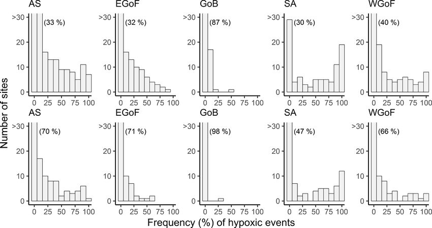
3186                                                           E. A. Virtanen et al.: Identifying areas prone to coastal hypoxia

the decay of wave exposure with depth and takes into ac-                 Ideal model tuning parameters (learning rate, bag frac-
count the diffraction and refraction of waves around islands         tion, tree complexity) for our hypoxia models were based
(Bekkby et al., 2008). SWM(d) characterizes areas where              on optimizing the model performance, i.e., minimizing the
water movement is slower, i.e., where water resides longer.          prediction error. The learning rate was set to 0.001 to de-
In terrestrial realms, landform influences on windthrow pat-         termine the contribution of each successive tree to the final
terns, i.e., exposure to winds, have been noted in several           model. We varied the number of decision rules controlling
studies, e.g., Kramer (2001) and Ashcroft et al (2008). Here,        model interaction levels, i.e., tree complexities, between 3
we introduce an analogous version of windthrow-prone areas           and 6. We shuffled the hypoxia data randomly into 10 sub-
to the marine realm, i.e., a wave-prone metric: topographic          sets for training (70 %) and testing (30 %) while preserving
shelter index (TSI), which differentiates wave directions and        the prevalence ratio of hypoxia occurrence. Hypoxia mod-
takes into account the sheltering effects of islands (i.e., ex-      els were developed based on 10-fold cross-validation, and
posure above sea level). The identification of wave-prone            the resulting final, best models leading to the smallest pre-
areas was calculated for the azimuths multiple of 15 (0–             dictive errors were chosen to predict the probability of de-
345◦ ) and for altitudes (corresponding to the angle of light        tecting hypoxia across the study region at a resolution of
source) ranging from 0.125 to 81◦ . For each altitude the pro-       20 m. We believe such a high resolution is necessary due to
duced wave-prone areas were combined to an index value for           the complexity of the archipelagoes of Finland and Sweden.
each grid cell. Surface roughness is a commonly used mea-            Model predictions for the whole seascape were repeated 10
sure of topographical complexity in terrestrial studies and          times with different model fits from data subsets (40 separate
has been used in marine realms as well (see, e.g., Dunn and          model predictions) to identify areas where models agree on
Halpin, 2009, for modeling habitats of hard substrates and           the area to be potentially hypoxic. Model performances were
Walker et al., 2009, for complexity of coral reef habitats).         estimated against the independent data (test data 30 %), not
Here, we consider two approaches for estimating seascape             used in model fitting in order to evaluate the potential over-
rugosity: arc-chord rugosity (ACR) and vector ruggedness             fitting of the models. Analyses were performed in R 3.5.0
measure (VRM). ACR is a landscape metrics, which evalu-              (R Core Team, 2018) with R libraries gbm (Greenwell et al.,
ates surface ruggedness using a ratio of contoured area (sur-        2018), PresenceAbsence (Freeman and Moisen, 2008) and
face area) to the area of a plane of best fit, which is a function   relevant functions from Elith et al. (2008).
of the boundary data (Du Preez, 2015). VRM, on the other                 Variable selection in BRT is internal by including only rel-
hand, is a more conservative measure of surface roughness            evant predictors when building models. The importance of
developed for wildlife habitat models and is calculated using        predictors is based on the time each predictor is chosen in
a moving 3×3 window where a unit vector orthogonal to the            each split, averaged over all trees. Higher scores (summed
cell is decomposed using the three-dimensional location of           up to 100 %) indicate that a predictor has a strong influence
the cell center, the local slope and aspect. A resultant vec-        on the response (Elith et al., 2008). Although BRT is not sen-
tor is divided by the number of cells in the moving window           sitive to collinearity of predictors, the ability to identify the
(Sappington et al., 2007). Both rugosity indices were used           strongest predictors by decreasing the estimated importance
here to identify areas with complex marine geomorphology.            score of highly correlated ones is detrimental to the inter-
Differences of predictor variables are illustrated in Fig. 2. We     pretability of models (Gregorutti et al., 2017). Selecting only
also included geographical study areas as predictors, in order       an optimal and a minimal set of variables for modeling, i.e.,
to highlight the differences between WFD areas.                      finding all relevant predictors and keeping the number of pre-
                                                                     dictors as small as possible, reduces the risk of overfitting
2.4    Hypoxia models                                                and improves the model accuracy. Here, most of the predic-
                                                                     tors describe the seascape structure and are somehow related
Based on the ecologically meaningful limits of hypoxia (see          to the topography of the seabed. We estimated the potential
Sect. 2.2), we built four separate oxygen models based on            to drop redundant predictors, i.e., those that would lead to
frequency and severity of hypoxia: occasional with O2 lim-           marked improvement in model performance if left out from
its < 4.6 and < 2 mg L−1 (hereafter referred to as OH4.6             the model building. For this, we used internal backward fea-
and OH2 ) and frequent hypoxia with O2 limits < 4.6 and              ture selection in BRT. However, we did not find marked dif-
< 2 mg L−1 (hereafter referred to as FH4.6 and FH2 ). We used        ferences in predictive performances and used all predictors.
the generalized boosted regression model (GBM) and its ex-               Estimation of model fits and predictive performances was
tension boosted regression trees (BRTs), a method from sta-          based on the ability to discriminate a hypoxic site from an
tistical and machine learning traditions (De’ath and Fabri-          oxic one, evaluated with the area under the curve (AUC)
cius, 2000; Hastie et al., 2001; Schapire, 2003). BRT opti-          (Jiménez-Valverde and Lobo, 2007) and simply with the per-
mizes predictive performance through integrated stochastic           cent correctly classified (PCC) (Freeman and Moisen, 2008).
gradient boosting (Natekin and Knoll, 2013) and forms the            AUC is a measure of the detection accuracy of true positives
best model for prediction based on several models.                   (sensitivity) and true negatives (specificity), and AUC values

Biogeosciences, 16, 3183–3195, 2019                                                       www.biogeosciences.net/16/3183/2019/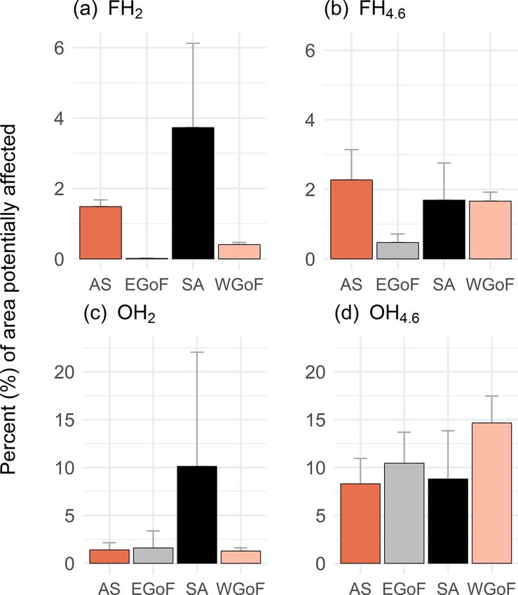
E. A. Virtanen et al.: Identifying areas prone to coastal hypoxia                                                                3187

Figure 2. Predictor variables developed for hypoxia ensemble models: (a) vector ruggedness measure (VRM), (b) depth-attenuated wave
exposure (SWM(d)), (c) topographic shelter index (TSI) and (d) bathymetric position index (BPI) with a search radius of 2 km. Red color
represents rugged seafloors (VRM), sheltered areas (SWM(d), TSI) and depressions (BPI2). Islands are shown as white.

above 0.9 indicate excellent, of 0.7–0.9 indicate good and            et al., 2005). Here, we define thresholds objectively based
below 0.7 indicate poor predictions.                                  on an agreement between predicted and observed hypoxia
   We transformed hypoxia probability predictions into bi-            prevalence. This approach underestimates areas potentially
nary classes of presence/absence and estimated the relative           hypoxic (see Sect. 3.4) and is expressed here as a conserva-
area of potentially hypoxic waters due to topographical rea-          tive estimate.
sons. Although dichotomization of probability predictions
flattens the information content, it facilitates the interpreta-
tion of results and is needed for management purposes. The            3     Results
predicted range of hypoxia and the potential geographical ex-
tent enables the identification of problematic areas and fa-          3.1    Hypoxia in complex coastal archipelagos
cilitates management actions in a cost-effective way. There
                                                                      During 2000–2016 hypoxia was rather common through-
are various approaches for determining thresholds, which are
                                                                      out the whole study region. In Finland, hypoxia mostly oc-
based on the confusion matrix, i.e., how well the model cap-
                                                                      curred on the southern coast, as in the Archipelago Sea (AS),
tures true/false presences or true/false absences. Usually the
                                                                      eastern Gulf of Finland (EGoF) and western Gulf of Fin-
threshold is defined to maximize the agreement between ob-
                                                                      land (WGoF) hypoxic events were recorded frequently. Only
served and predicted distributions. Widely used thresholds,
                                                                      ∼ 30 % of coastal monitoring sites in AS, EGoF and SA were
such as 0.5, can be arbitrary unless the threshold equals
                                                                      not hypoxic; i.e., oxygen concentrations were always above
prevalence of presences in the data, i.e., the frequency of
                                                                      4.6 mg L−1 (see percentages in brackets in Fig. 3). Coastal
occurrences (how many presences of the total dataset) (Liu
                                                                      areas in the Stockholm archipelago (SA) were also regularly

www.biogeosciences.net/16/3183/2019/                                                          Biogeosciences, 16, 3183–3195, 2019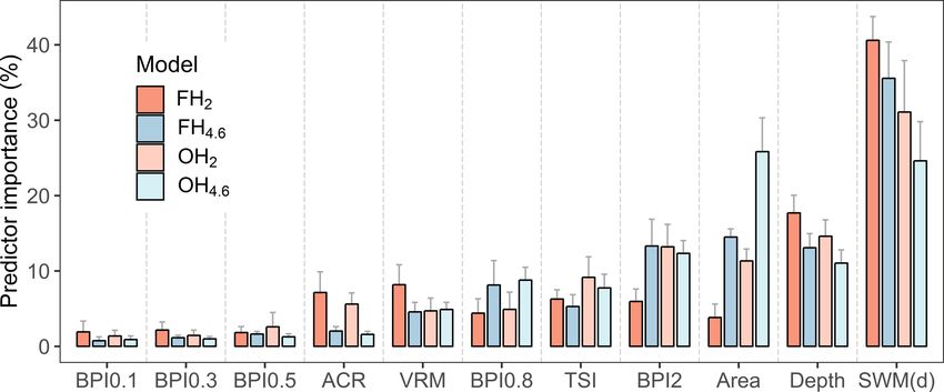
3188                                                         E. A. Virtanen et al.: Identifying areas prone to coastal hypoxia

hypoxic, with 70 % of the sites moderately (O2 < 4.6 mg L−1 )      3.4    Hypoxic areas
and 53 % severely (O2 < 2 mg L−1 ) hypoxic. Severe hypoxia
was quite a localized phenomenon in Finland, as it was             Although hypoxia was commonly recorded in all WFD ar-
recorded at ca. 30 % of sites in AS and EGoF. However, in          eas, except in the Gulf of Bothnia, the potential geographi-
WGoF there are sites where severe hypoxia is rather persis-        cal extent of hypoxic seafloors shows a rather different pat-
tent, as every sampling event was recorded as hypoxic. The         tern. Based on models, topographically prone areas represent
same applies to SA, as there are quite a few sites repeat-         only a small part of the coastal areas, with less than 25 %
edly severely hypoxic. In contrast, in the northern study area,    affected (Fig. 6). Frequent, severe hypoxia (O2 < 2 mg L−1 )
Gulf of Bothnia (GoB), hypoxic events occurred rather infre-       was most prominent in the Archipelago Sea and Stockholm
quently, as in 98 % of sites O2 was above 2 mg L−1 and in          archipelago, although representing only a small fraction of
87 % O2 was above 4.6 mg L−1 (Fig. 3).                             the total areas (on average 1.5 % and 3.7 %, respectively).
                                                                   Problematic areas based on the models are the Archipelago
                                                                   Sea, Stockholm archipelago and western Gulf of Finland.
3.2    Importance of predictors                                    Those areas seem to be topographically prone to oxygen de-
                                                                   ficiency. Moreover, around 10 % of areas in the eastern Gulf
Models developed on 566 sites, based on 10-fold cross-             of Finland are vulnerable to occasional moderate hypoxia but
validation and 10 repeated predictions; the most influential       less to severe hypoxia. Areas predicted as hypoxic in the Gulf
predictor (averaged across models) was SWM(d), with a              of Bothnia were less than < 2 %, which supports our hypothe-
mean contribution of 33 % (±5 %) (Fig. 4). The contribu-           sis of the facilitating role that topography potential has. There
tion of SWM(d) was highest for frequent, severe hypoxia            are fewer depressions (Supplement Fig. S1), and the seafloor
(FH2 ) (41 ± 3 %), whereas for occasional, moderate hypoxia        is topographically less complex than in the other study areas.
(OH4.6 ) the influence was markedly lower (25 ± 5 %). This
supports the hypothesis that in sheltered areas, where water
movement is limited, severe oxygen deficiency is likely to         4     Discussion
develop. It is also noteworthy that depth was not the most im-
portant driver of hypoxia in coastal areas. This suggests that     Hypoxia has been increasing steadily since the 1960s, and
coastal hypoxia is not directly dependent on depth but that        anoxic areas are seizing the seafloor, suffocating marine
depressions that are especially steep and isolated are more        organisms in the way (Diaz and Rosenberg, 2008; Breit-
sheltered and become more easily hypoxic than smoother de-         burg et al., 2018). Understanding the factors affecting the
pressions.                                                         severity and spatial extent of hypoxia is essential in or-
   Across models, BPIs identifying wider sinks (BPI2 and           der to estimate rates of deoxygenation and its consequences
BPI0.8) were more influential than BPIs identifying smaller        to the marine ecosystems (Breitburg et al., 2018). Earlier
sinks (BPIs 0.1, 0.3 and 0.5), and terrain ruggedness mea-         studies have reported coastal hypoxia to be a global phe-
sures, VRM and ACR, were more important for frequent               nomenon (Diaz and Rosenberg, 2008; Conley et al., 2011)
severe hypoxia (FH2 ) than for moderate hypoxia (FH4.6 ).          and is known to be widespread in the Baltic Sea (Conley
The relatively high contribution of topographic shelter (TSI       et al., 2011). Our results confirmed this and showed that
7 ± 2 %) indicates that, in areas where there are higher is-       coastal hypoxia is perhaps a more common phenomenon
lands, the basins between are prone to hypoxia formation.          than previously anticipated. According to our results, over
                                                                   50 % of sites in the complex archipelagoes of Finland and
                                                                   Sweden experienced hypoxia that is ecologically signifi-
3.3    Model performance
                                                                   cant (O2 < 4.6 mg L−1 ). Especially alarming was the inten-
                                                                   sity of it. For instance, the Stockholm archipelago suffered
Predictive ability of models to detect sites as hypoxic across     frequently from severe hypoxia (O2 < 2 mg L−1 ), as approx-
models was good, with a mean 10-fold cross-validated AUC           imately half of the coastal monitoring sites were hypoxic
of 0.85 (±0.02) and mean AUC of 0.86 (±0.03) when evalu-           across our study period (Fig. 3). This demonstrates that de-
ated against independent test data for 242 sites (30 % of sites)   oxygenated seafloors are probably even more common in
(Fig. 5a). Models classified on average 88 % of sites correctly    coastal environments than previously reported (Karlsson et
(PCCcv in Fig. 5b) and performed only slightly worse when          al., 2010; Conley et al., 2011). It is notable that in areas above
evaluated against independent data, with 81 % (±3 %) cor-          the permanent halocline, hypoxia is in many areas seasonal
rectly classified (PCCin in Fig. 5b). Models developed for         and develops after the building of thermocline in late summer
frequent hypoxia (FH2 and FH4.6 ) were better (mean AUCin          (Conley et al., 2011). It is therefore probable that many of
0.88 ± 0.03) compared to occasional hypoxia models (mean           the areas we recognized as hypoxic may well be oxygenated
AUCin 0.84 ± 0.04). This suggests that other factors beyond        during winter and spring. This does not however reduce the
topographical proxies contribute relatively more to the oc-        severity of the phenomenon. Even a hypoxic event of short
currence of occasional hypoxia than for frequent hypoxia.          duration, e.g., a few days, will reduce ecosystem resistance

Biogeosciences, 16, 3183–3195, 2019                                                     www.biogeosciences.net/16/3183/2019/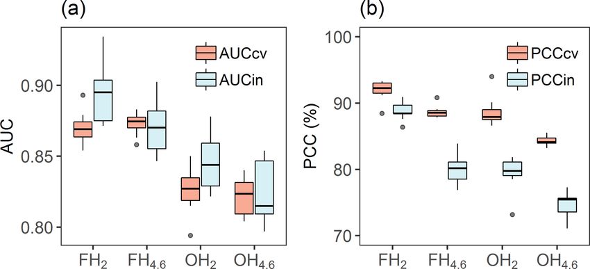
E. A. Virtanen et al.: Identifying areas prone to coastal hypoxia                                                                  3189

Figure 3. Frequencies of hypoxic events at coastal monitoring sites across Water Framework Directive areas: Archipelago Sea (AS), eastern
Gulf of Finland (EGoF), Gulf of Bothnia (GoB), Stockholm archipelago (SA) and western Gulf of Finland (WGoF). Upper panels indicate
O2 < 4.6 mg L−1 and lower panels O2 < 2 mg L−1 . Numbers in brackets indicate the percentage of sites with O2 > 4.6 (upper panel) and
O2 > 2 mg L−1 (lower panel). Number of sites over 30 are not shown.

Figure 4. Importance of predictors based on 10 prediction rounds. Predictors are color-coded based on models. FH2 : frequent, severe
hypoxia (O2 < 2 mg L−1 ); FH4.6 : frequent, moderate hypoxia (O2 < 4.6 mg L−1 ); OH2 : occasional, severe hypoxia (O2 < 2 mg L−1 ), and
OH4.6 : occasional, moderate hypoxia (O2 < 4.6 mg L−1 ). Whiskers represent standard deviations.

to further hypoxic perturbation and affect the overall ecosys-            Although extensive 3-D models have been developed for
tem functioning (Villnas et al., 2013).                                the main basins of the Baltic Sea (Meier et al., 2011b, 2012a,
   As our study suggests, topographically prone areas to de-           2014) the previous reports on the occurrence of coastal hy-
oxygenation represent less than 25 % of seascapes. However,            poxia have mostly been based on point observations (Conley
most of the underwater nature values in the Finnish sea areas          et al., 2009, 2011). Due to the lack of data, and computational
are concentrated on relatively shallow areas where there ex-           limitations, no biogeochemical model has (yet) encompassed
ist enough light and suitable substrates (Virtanen et al., 2018;       the complex Baltic Sea archipelago with a resolution needed
Lappalainen et al., 2019). Shallow areas also suffer from eu-          for adjusting local management decisions. This study pro-
trophication and rising temperatures due to changing climate           vides a novel methodology to predict and identify areas prone
and are most probably the ones that are particularly suscep-           to coastal hypoxia without data on currents, stratification or
tible to hypoxia in the future (Breitburg et al., 2018). This          biological variables, and without complex biogeochemical
suggests that seasonal hypoxia may become a recurrent phe-             models. Our approach is applicable to other low-energy and
nomenon in shallow areas above the thermocline in late sum-            nontidal systems, such as large shallow bays and semien-
mer.                                                                   closed or enclosed sea areas. The benefit of this approach is
                                                                       that it requires far less computational power than a fine-scale

www.biogeosciences.net/16/3183/2019/                                                           Biogeosciences, 16, 3183–3195, 2019
3190 E. A. Virtanen et al.: Identifying areas prone to coastal hypoxia
Figure 5. Model performances based on (a) area under the curve
values with 10-fold cross-validation (AUCcv ) and against indepen-
dent test data (30 % of sites) (AUCin ) as well as (b) percent of cor-
rectly classified with 10-fold cross-validation (PCCcv ) and against
independent data (PCCin ).
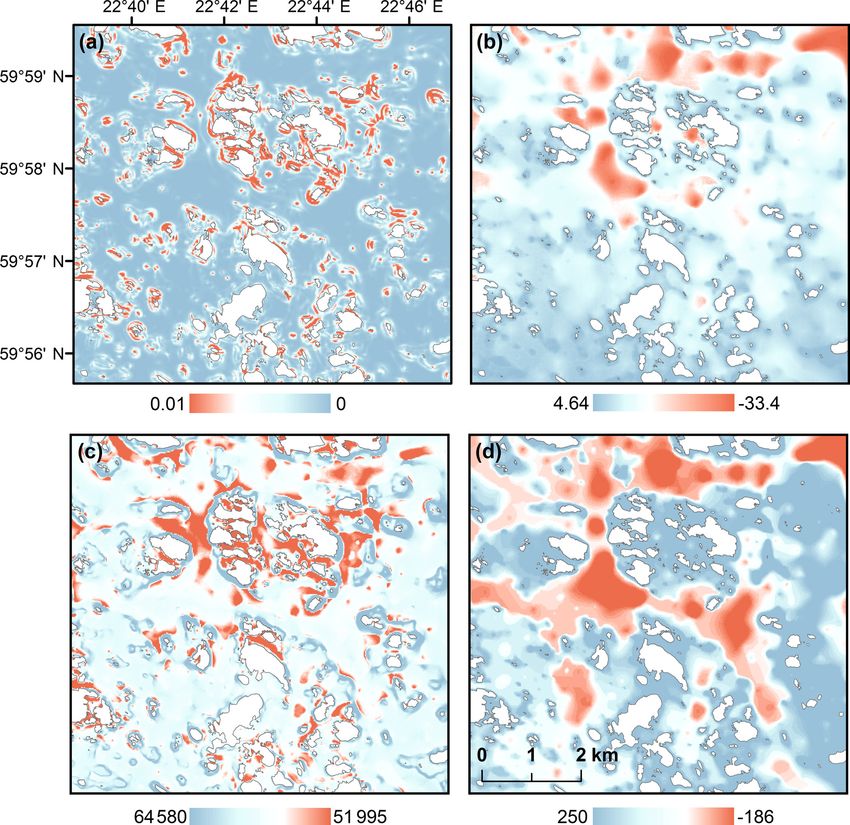
Figure 7. Modeled probability (%) of detecting frequent hypoxia
O2 (< 4.6 mg L−1 ) due to topography in an example area off the
southern coast of Finland. Land shown as white color.
erogeneous areas, where water exchange is limited, are more
susceptible to developing hypoxia according to our results.
This statement is quite intuitive, but it has not previously
been quantified. It is also noteworthy that coastal hypoxia
is not only related to depth; deep seafloors are not automati-
cally hypoxic or anoxic. In our study, hypoxia was common
in shallow and moderate depths of 10–45 m. For instance,
in the Archipelago Sea, deep (60–100 m) channels are not
usually hypoxic, as strong currents tend to keep them oxy-
genated throughout the year (Virtasalo et al., 2005). Shallow
areas can be restricted by slow water movement due to to-
pographical reasons, thus creating opportunities for hypoxia
formation.
We emphasize that our models only indicate where hy-
poxia may occur simply due to restricted water exchange.
Any deviations from this pattern are probably caused by ei-
ther hydrographic factors, which the hypoxia model based
on topography did not account for (such as strong currents
in elongated, wide channels), or biogeochemical factors. Es-
Figure 6. Percent (%) of areas potentially affected by hypoxia with pecially high external loading, and local biogeochemical and
varying frequencies (occasional and frequent) and hypoxia sever- biological processes (nutrient cycling between sediment and
ities (O2 < 4.6 and O2 < 2 mg L−1 ). AS: Archipelago Sea; EGoF: the water), obviously modifies the patterns and severity of
eastern Gulf of Finland; SA: Stockholm archipelago; and WGoF: hypoxia also in the coastal areas. Oxygen deficiency has been
western Gulf of Finland. GoB is not reported as areas potentially projected to increase faster in the coastal systems than in the
affected were below 2 % across all models. open sea (Gilbert et al., 2010; Altieri and Gedan, 2015). Such
coastal areas are usually affected by external nutrient loading
from the watershed. In larger basins and sea areas dominated
3-D numerical modeling. By using relatively simple prox- by large river systems, such as the central Baltic Sea, Gulf
ies describing depressions of stagnant water, we were able to of Mexico and Chesapeake Bay, large-scale oceanographic
create detailed hypoxia maps for the entire Finnish coastal and biogeochemical processes, or external loading, govern
area (23 500 km2 ) and Stockholm archipelago (5100 km2 ), the depth and extent of hypoxia. This is the case also in the
thus enabling a quick view of potentially hypoxic waters Baltic Sea. In areas where our models underestimate oxygen
(Fig. 7). deficiency, major nutrient sources, e.g., rivers, cities or inten-
We quantified the facilitating role of seafloor complexity sive agricultural areas, probably contribute to hypoxia for-
for the formation of hypoxia. Sheltered, topographically het- mation. However, in extremely complex archipelago areas,
Biogeosciences, 16, 3183–3195, 2019 www.biogeosciences.net/16/3183/2019/E. A. Virtanen et al.: Identifying areas prone to coastal hypoxia 3191
such as the Finnish and Swedish archipelago, physical fac- In the Gulf of Bothnia, hypoxia was markedly less fre-
tors limiting lateral and vertical movement of water probably quent and severe than in the other study areas. GoB has a rel-
facilitate, and in some areas even dictate, the development of atively open coastline with only few depressions (see Fig. S1)
hypoxia. and strong wave forcing, which probably enhances the mix-
There were spatial differences in the frequency and sever- ing of water in the coastal areas. Moreover, as the open-sea
ity of hypoxia that can be explained by topographical char- areas of the Gulf of Bothnia are well oxygenated due to a
acteristics of the areas, external loading and interaction with lack of halocline and topographical isolation of GoB from the
the adjacent deeper basins. For instance, in the Stockholm Baltic Proper (by the sill between these basins) (Leppäranta
archipelago severe hypoxia covered the largest percentage of and Myrberg, 2009), hypoxic water is not advected from the
seascapes of all study areas. The Stockholm archipelago is open sea to the coastal areas.
part of a joint valley landscape with deep, steep areas also in Such observations suggest that formation of coastal hy-
the inner parts where wave forcing is exceptionally low and poxia is not totally independent from basin-scale oxygen dy-
disconnected from the open sea, making it very susceptible to namics. While we suggest that coastal hypoxia can be formed
hypoxia, which was also confirmed by the model. In Finland, entirely based on local morphology and local biogeochemi-
the inner archipelago is mostly shallow, with steep but wider cal processes, the relatively low occurrence of hypoxia in the
channels occurring only in the Archipelago Sea. These elon- Gulf of Bothnia and differences in frequency of hypoxia in
gated channels are connected to adjacent open-sea areas and different parts of the Gulf of Finland both highlight the inter-
thus well-ventilated, as opposed to the narrow channels of action of these coastal areas with the Baltic Proper.
the Stockholm archipelago. Geographically, hypoxia in Fin- While our results confirm that hypoxia in most study ar-
land was most prominent in the Archipelago Sea and the Gulf eas is a frequently occurring phenomenon, they also show
of Finland, where the inner archipelago is isolated from the that areas affected by hypoxia are geographically still lim-
open sea, and the complex topography results in overall poor ited. Our modeling results indicate that, overall, less than
water exchange in the existing depressions. Both the Stock- 25 % of the studied sea areas were afflicted by some form
holm archipelago and the Archipelago Sea suffer from exter- of hypoxia (be it recurrent or occasional), and less than 6 %
nal loading from the associated watersheds and internal load- of seascapes were plagued by frequent, severe hypoxia. The
ing from sediments, which probably contributes to the poor relatively small spatial extent of coastal hypoxia does not
oxygen status of these areas (Puttonen et al., 2014; Walve mean that it is not a harmful phenomenon. In the Stockholm
et al., 2018). Biogeochemical factors were however not ac- archipelago, severe hypoxia is a pervasive and persistent phe-
counted for by our analysis and cannot be used in explaining nomenon, and also in Finland, many local depressions are
the observed spatial differences. often hypoxic. Anoxic local depressions probably act as lo-
In the Gulf of Finland, eutrophication increases in the cal nutrient sources, releasing especially phosphorus to the
open sea from west to east, which has traditionally been ex- water column, which further enhances pelagic primary pro-
plained by nutrient discharges from the Neva River (HEL- duction. Such a vicious circle tends to worsen the eutrophica-
COM, 2018). In our data there was however no clear gradi- tion and maintain the environment in a poor state (Pitkänen
ent of coastal hypoxia increasing towards east. In contrast, et al., 2001; Vahtera et al., 2007). In this way, even small-
frequent hypoxia was more common in the Archipelago Sea sized anoxic depressions, especially if they are many, may
and western Gulf of Finland than in the eastern Gulf of Fin- affect the ecological status of the whole coastal area. More-
land, where hypoxia occurred only occasionally. This sug- over, as climate change has been projected to increase water
gests that the coastal hypoxia is more dependent on local pro- temperatures and worsen hypoxia in the Baltic Sea (Meier
cesses, i.e., internal loading and external loading from nearby et al., 2011a), shallow archipelago areas that typically have
areas, whereas open-sea hypoxia is governed by basin-scale high productivity, warm up quickly and are topographically
dynamics. However, the occasional nature of hypoxia in the prone to hypoxia may be especially vulnerable to the nega-
eastern Gulf of Finland may be at least partly caused by the tive effects of climate change.
dependency on the deep waters of the open parts of the Gulf In order to establish reference conditions and implement
of Finland. The Gulf of Finland is an embayment, 400 km necessary and cost-efficient measures to reach the goals of in-
long and 50–120 km wide, which has an open western bound- ternational agreements such as the EU Water Framework Di-
ary to the Baltic Proper. A tongue of anoxic water usually rective (WFD, 2000/60/EC), the Marine Strategy Framework
extends from the central Baltic Sea into the Gulf of Finland Directive (MSFD, 2008/56/EC) and the HELCOM Baltic
along its deepest parts. Basin-scale oceanographic and atmo- Sea Action Plan (BSAP), in-depth knowledge of ecological
spheric processes influence how far east this tongue proceeds functions and processes as well as natural preconditions is
into the Gulf of Finland each year (Alenius et al., 2016). It is needed. Although eutrophication is a problem for the whole
possible that, when this anoxic tongue extends close to east- Baltic Sea, nutrient abatement measures are taken locally.
ern Gulf of Finland, it also worsens the oxygen situation of We therefore need to know where the environmental bene-
the EGoF archipelago. fits are maximized and where natural conditions are likely
to counteract any measures taken. As some places are natu-
www.biogeosciences.net/16/3183/2019/ Biogeosciences, 16, 3183–3195, 20193192 E. A. Virtanen et al.: Identifying areas prone to coastal hypoxia
rally prone to hypoxia, our model could aid directing mea- Author contributions. EAV and MV designed the study, EAV and
sures to places where they are most likely to be efficient, as ANS performed all analyses, EAV wrote the main text, and all au-
well as explain why in some areas implemented measures do thors contributed to the writing and editing of the manuscript.
not have the desired effect. Our approach could be used to
develop an early-warning system for identification of areas
prone to oxygen loss and to indicate where eutrophication Competing interests. The authors declare that they have no conflict
mitigation actions are most urgently needed. of interest.
Acknowledgements. Elina A. Virtanen and Markku Viitasalo ac-
5 Conclusions knowledge the SmartSea project (grant nos. 292985 and 314225),
funded by the Strategic Research Council of the Academy of Fin-
While biogeochemical 3-D models have been able to accu- land, and the Finnish Inventory Programme for the Underwater Ma-
rately project basin-scale oxygen dynamics, describing spa- rine Environment VELMU, funded by the Ministry of the Envi-
tial variation of hypoxia in coastal areas has remained a chal- ronment. Alf Norkko acknowledges the support of the Academy of
lenge. Recognizing that the enclosed nature of seafloors con- Finland (no. 294853) and the Sophie von Julins Foundation. Anto-
nia Nyström Sandman acknowledges the IMAGINE project (grant
tributes to hypoxia formation, we used simple topographical
no. 15/247), funded by the Swedish EPA. We wish to thank two
parameters to model the occurrence of hypoxia in the com- anonymous reviewers for insightful comments that significantly im-
plex Finnish and Swedish archipelagoes. We found that a proved the manuscript.
surprisingly large fraction (∼ 80 %) of hypoxia occurrences
could be explained by topographical parameters alone. Mod-
eling results also suggested that less than 25 % of the studied Financial support. This research has been supported by the Strate-
seascapes were prone to hypoxia during late summer. Large gic Research Council of the Academy of Finland (SmartSea project)
variation existed in the spatial and temporal patterns of hy- (grant nos. 292985 and 314225), the Ministry of the Environment
poxia, however, with certain areas being prone to occasional (the Finnish Inventory Programme for the Underwater Marine En-
severe hypoxia (O2 < 2 mg L−1 ), while others were more sus- vironment VELMU), the Academy of Finland (grant no. 294853),
ceptible to recurrent moderate hypoxia (O2 < 4.6 mg L−1 ). and the Swedish EPA (IMAGINE project) (grant no. 15/247).
Sheltered, topographically heterogeneous areas with limited
water exchange were susceptible to developing hypoxia, in
contrast to less sheltered areas with high wave forcing. In Review statement. This paper was edited by Carol Robinson and
some areas oxygen conditions were either better or worse reviewed by two anonymous referees.
than predicted by the model. We assume that these devi-
ations from the topographical background were caused by
processes not accounted for by the model, such as hydro-
References
graphical processes, e.g., strong currents causing improved
mixing, or by high external or internal nutrient loading, in- Alenius, P., Myrberg, K., Roiha, P., Lips, U., Tuomi, L., Petters-
ducing high local oxygen consumption. We conclude that son, H., and Raateoja, M.: Gulf of Finland Physics, in: The Gulf
formation of coastal hypoxia is probably primarily dictated of Finland assessment, edited by: Raateoja, M. and Setälä, O.,
by local processes, and can be quite accurately projected Helsinki, Finnish Environment Institute, Reports of the Finnish
using simple topographical parameters, but that interaction Environment Institute, 27, 42–57, 2016.
with the associated watershed and the adjacent deeper basins Altieri, A. H. and Gedan, K. B.: Climate change and
of the Baltic Sea can also influence local oxygen dynamics dead zones, Glob. Change Biol., 21, 1395–1406,
in many areas. Our approach gives a practical baseline for https://doi.org/10.1111/gcb.12754, 2015.
various types of hypoxia-related studies and, consequently, Ashcroft, M. B., Chisholm, L. A., and French, K. O.: The ef-
fect of exposure on landscape scale soil surface temperatures
decision-making. Identifying areas prone to hypoxia helps to
and species distribution models, Landscape Ecol., 23, 211–225,
focus research, management and conservation actions in a https://doi.org/10.1007/s10980-007-9181-8, 2008.
cost-effective way. Bekkby, T., Isachsen, P. E., Isaeus, M., and Bakkestuen, V.:
GIS modeling of wave exposure at the seabed: A depth-
attenuated wave exposure model, Mar. Geod., 31, 117–127,
Data availability. Hypoxia point data and scripts for reproducing https://doi.org/10.1080/01490410802053674, 2008.
the models and plots are available at the Dryad data repository: Greenwell, B., Boehmke, B., Cunningham, J., and GBM De-
https://doi.org/10.5061/dryad.cn5kh5m (Virtanen et al., 2019). velopers: gbm: Generalized Boosted Regression Models, R
package version 2.1.4, available at: https://CRAN.R-project.org/
package=gbm (last access: 11 March 2019), 2018.
Supplement. The supplement related to this article is available on- Breitburg, D., Levin, L. A., Oschlies, A., Grégoire, M., Chavez, F.
line at: https://doi.org/10.5194/bg-16-3183-2019-supplement. P., Conley, D. J., Garçon, V., Gilbert, D., Gutiérrez, D., Isensee,
Biogeosciences, 16, 3183–3195, 2019 www.biogeosciences.net/16/3183/2019/E. A. Virtanen et al.: Identifying areas prone to coastal hypoxia 3193 K., Jacinto, G. S., Limburg, K. E., Montes, I., Naqvi, S. W. A., Baltic Sea; A model study, J. Mar. Syst., 75, 163–184, Pitcher, G. C., Rabalais, N. N., Roman, M. R., Rose, K. A., https://doi.org/10.1016/j.jmarsys.2008.08.009, 2009. Seibel, B. A., Telszewski, M., Yasuhara, M., and Zhang, J.: De- Eilola, K., Gustafsson, B. G., Kuznetsov, I., Meier, H. E. M., clining oxygen in the global ocean and coastal waters, Science, Neumann, T., and Savchuk, O. P.: Evaluation of biogeochem- 359, 1–11, https://doi.org/10.1126/science.aam7240, 2018. ical cycles in an ensemble of three state-of-the-art numeri- Buzzelli, C. P., Luettich Jr, R. A., Powers, S. P., Peterson, C. H., cal models of the Baltic Sea, J. Mar. Syst., 88, 267–284, McNinch, J. E., Pinckney, J. L., and Paerl, H. W.: Estimating the https://doi.org/10.1016/j.jmarsys.2011.05.004, 2011. spatial extent of bottom-water hypoxia and habitat degradation Elith, J., Leathwick, J. R., and Hastie, T.: A working guide in a shallow estuary, Mar. Ecol. Prog. Ser., 230, 103–112, 2002. to boosted regression trees, J. Anim. Ecol., 77, 802–813, Caballero-Alfonso, A. M., Carstensen, J., and Con- https://doi.org/10.1111/j.1365-2656.2008.01390.x, 2008. ley, D. J.: Biogeochemical and environmental drivers Eriksson, S. P., Wennhage, H., Norkko, J., and Norkko, A.: of coastal hypoxia, J. Mar. Syst., 141, 190–199, Episodic disturbance events modify predator-prey interactions https://doi.org/10.1016/j.jmarsys.2014.04.008, 2015. in soft sediments, Estuar. Coast. Shelf S., 64, 289–294, Carstensen, J., Andersen, J. H., Gustafsson, B. G., and Con- https://doi.org/10.1016/j.ecss.2005.02.022, 2005. ley, D. J.: Deoxygenation of the Baltic Sea during the Fennel, K. and Testa, J. M.: Biogeochemical Controls on last century, P. Natl. Acad. Sci. USA, 111, 5628–5633, Coastal Hypoxia, Annu. Rev. Mar. Sci., 11, 105–130, https://doi.org/10.1073/pnas.1323156111, 2014. https://doi.org/10.1146/annurev-marine-010318-095138, 2019. Conley, D. J., Humborg, C., Rahm, L., Savchuk, O. P., and Wulff, Fennel, K., Hetland, R., Feng, Y., and DiMarco, S.: A cou- F.: Hypoxia in the Baltic Sea and basin-scale changes in phos- pled physical-biological model of the Northern Gulf of phorus biogeochemistry, Environ. Sci. Technol., 36, 5315–5320, Mexico shelf: model description, validation and analysis https://doi.org/10.1021/es025763w, 2002. of phytoplankton variability, Biogeosciences, 8, 1881–1899, Conley, D. J., Björck, S., Bonsdorff, E., Carstensen, J., Destouni, https://doi.org/10.5194/bg-8-1881-2011, 2011. G., Gustafsson, B. G., Hietanen, S., Kortekaas, M., Kuosa, H., Fennel, K., Laurent, A., Hetland, R., Justic, D., Ko, D. S., Lehrter, Markus Meier, H. E., Müller-Karulis, B., Nordberg, K., Norkko, J., Murrell, M., Wang, L. X., Yu, L. Q., and Zhang, W. X.: Effects A., Nürnberg, G., Pitkänen, H., Rabalais, N. N., Rosenberg, R., of model physics on hypoxia simulations for the northern Gulf Savchuk, O. P., Slomp, C. P., Voss, M., Wulff, F., and Zillén, L.: of Mexico: A model intercomparison, J. Geophys. Res.-Ocean., Hypoxia-Related Processes in the Baltic Sea, Environ. Sci. Tech- 121, 5731–5750, https://doi.org/10.1002/2015jc011577, 2016. nol., 43, 3412–3420, https://doi.org/10.1021/es802762a, 2009. Freeman, E. A. and Moisen, G.: PresenceAbsence: An R Package Conley, D. J., Carstensen, J., Aigars, J., Axe, P., Bonsdorff, E., for Presence-Absence Model Analysis, J. Stat. Softw., 23, 1–31, Eremina, T., Haahti, B. M., Humborg, C., Jonsson, P., Kotta, 2008. J., Lannegren, C., Larsson, U., Maximov, A., Medina, M. R., Frölicher, T. L., Joos, F., Plattner, G. K., Steinacher, M., Lysiak-Pastuszak, E., Remeikaite-Nikiene, N., Walve, J., Wil- and Doney, S. C.: Natural variability and anthropogenic helms, S., and Zillen, L.: Hypoxia Is Increasing in the Coastal trends in oceanic oxygen in a coupled carbon cycle– Zone of the Baltic Sea, Environ. Sci. Technol., 45, 6777–6783, climate model ensemble, Global Biogeochem. Cy., 23, 1–15, https://doi.org/10.1021/es201212r, 2011. https://doi.org/10.1029/2008GB003316, 2009. De’ath, G. and Fabricius, K. E.: Classification and regression Gammal, J., Norkko, J., Pilditch, C. A., and Norkko, A.: Coastal trees: A powerful yet simple technique for ecological data Hypoxia and the Importance of Benthic Macrofauna Commu- analysis, Ecology, 81, 3178–3192, https://doi.org/10.1890/0012- nities for Ecosystem Functioning, Estuar. Coast., 40, 457–468, 9658(2000)081[3178:CARTAP]2.0.CO;2, 2000. https://doi.org/10.1007/s12237-016-0152-7, 2017. Diaz, R. and Rosenberg, R.: Marine benthic hypoxia: A review of its Gilbert, D., Rabalais, N. N., Díaz, R. J., and Zhang, J.: ecological effects and the behavioural response of benthic macro- Evidence for greater oxygen decline rates in the coastal fauna, Oceanogr. Mar. Biol., 33, 245–303, 1995a. ocean than in the open ocean, Biogeosciences, 7, 2283–2296, Diaz, R. J. and Rosenberg, R.: Marine benthic hypoxia: A review https://doi.org/10.5194/bg-7-2283-2010, 2010. of its ecological effects and the behavioural responses of benthic Gray, J. S., Wu, R. S. S., and Or, Y. Y.: Effects of hypoxia and or- macrofauna, in: Oceanography and Marine Biology – an Annual ganic enrichment on the coastal marine environment, Mar. Ecol. Review, Vol. 33, edited by: Ansell, A. D., Gibson, R. N., and Prog. Ser., 238, 249–279, https://doi.org/10.3354/meps238249, Barnes, M., Oceanography and Marine Biology, U. C. L. Press 2002. Ltd, London, 245–303, 1995b. Gregorutti, B., Michel, B., and Saint-Pierre, P.: Correlation and vari- Diaz, R. J. and Rosenberg, R.: Spreading dead zones and con- able importance in random forests, Stat. Comput., 27, 659–678, sequences for marine ecosystems, Science, 321, 926–929, https://doi.org/10.1007/s11222-016-9646-1, 2017. https://doi.org/10.1126/science.1156401, 2008. Hastie, T., Tibshirani, R., and Friedman, J. H.: The Elements of Dunn, D. C. and Halpin, P. N.: Rugosity-based regional modeling Statistical Learning: Data Mining, Inference, and Prediction, of hard-bottom habitat, Mar. Ecol. Prog. Ser., 377, 1–11, 2009. Springer-Verlag, New York, 2001. Du Preez, C.: A new arc–chord ratio (ACR) rugosity index for HELCOM: Sources and pathways of nutrients to the Baltic Sea, quantifying three-dimensional landscape structural complexity, Baltic Sea Environment Proceedings No. 153, 1–48, 2018. Landscape Ecol., 30, 181–192, https://doi.org/10.1007/s10980- Hordoir, R., Axell, L., Höglund, A., Dieterich, C., Fransner, F., 014-0118-8, 2015. Gröger, M., Liu, Y., Pemberton, P., Schimanke, S., Andersson, Eilola, K., Meier, H. E. M., and Almroth, E.: On the dy- H., Ljungemyr, P., Nygren, P., Falahat, S., Nord, A., Jönsson, namics of oxygen, phosphorus and cyanobacteria in the A., Lake, I., Döös, K., Hieronymus, M., Dietze, H., Löptien, U., www.biogeosciences.net/16/3183/2019/ Biogeosciences, 16, 3183–3195, 2019
3194                                                             E. A. Virtanen et al.: Identifying areas prone to coastal hypoxia

   Kuznetsov, I., Westerlund, A., Tuomi, L., and Haapala, J.: Nemo-    Meier, H. E. M., Eilola, K., and Almroth, E.: Climate-related
   Nordic 1.0: a NEMO-based ocean model for the Baltic and North          changes in marine ecosystems simulated with a 3-dimensional
   seas – research and operational applications, Geosci. Model Dev.,      coupled physicalbiogeochemical model of the Baltic Sea, Clim.
   12, 363–386, https://doi.org/10.5194/gmd-12-363-2019, 2019.            Res., 48, 31–55, 2011b.
Jiménez-Valverde, A. and Lobo, J. M.: Threshold crite-                 Meier, H. E. M., Hordoir, R., Andersson, H. C., Dieterich, C.,
   ria for conversion of probability of species presence to               Eilola, K., Gustafsson, B. G., Hoglund, A., and Schimanke, S.:
   either–or presence–absence, Acta Oecol., 31, 361–369,                  Modeling the combined impact of changing climate and chang-
   https://doi.org/10.1016/j.actao.2007.02.001, 2007.                     ing nutrient loads on the Baltic Sea environment in an ensem-
Jokinen, S. A., Virtasalo, J. J., Jilbert, T., Kaiser, J., Dellwig,       ble of transient simulations for 1961–2099, Clim. Dynam., 39,
   O., Arz, H. W., Hänninen, J., Arppe, L., Collander, M., and            2421–2441, https://doi.org/10.1007/s00382-012-1339-7, 2012a.
   Saarinen, T.: A 1500-year multiproxy record of coastal hypoxia      Meier, H. E. M., Muller-Karulis, B., Andersson, H. C., Di-
   from the northern Baltic Sea indicates unprecedented deoxy-            eterich, C., Eilola, K., Gustafsson, B. G., Hoglund, A., Hor-
   genation over the 20th century, Biogeosciences, 15, 3975–4001,         doir, R., Kuznetsov, I., Neumann, T., Ranjbar, Z., Savchuk, O.
   https://doi.org/10.5194/bg-15-3975-2018, 2018.                         P., and Schimanke, S.: Impact of Climate Change on Ecologi-
Karlson, K., Rosenberg, R., and Bonsdorff, E.: Temporal and spatial       cal Quality Indicators and Biogeochemical Fluxes in the Baltic
   large-scale effects of eutrophication and oxygen deficiency on         Sea: A Multi-Model Ensemble Study, Ambio, 41, 558–573,
   benthic fauna in Scandinavian and Baltic waters – A review, in:        https://doi.org/10.1007/s13280-012-0320-3, 2012b.
   Oceanography and Marine Biology, Vol. 40, edited by: Gibson,        Meier, H. E. M., Andersson, H. C., Arheimer, B., Donnelly, C.,
   R. N., Barnes, M., and Atkinson, R. J. A., Oceanography and            Eilola, K., Gustafsson, B. G., Kotwicki, L., Neset, T.-S., Niira-
   Marine Biology, Taylor & Francis Ltd, London, 427–489, 2002.           nen, S., Piwowarczyk, J., Savchuk, O. P., Schenk, F., W˛esławski,
Karlsson, O. M., Jonsson, P. O., Lindgren, D., Malmaeus, J.               J. M., and Zorita, E.: Ensemble Modeling of the Baltic Sea
   M., and Stehn, A.: Indications of Recovery from Hypoxia                Ecosystem to Provide Scenarios for Management, Ambio, 43,
   in the Inner Stockholm Archipelago, Ambio, 39, 486–495,                37–48, https://doi.org/10.1007/s13280-013-0475-6, 2014.
   https://doi.org/10.1007/s13280-010-0079-3, 2010.                    Middelburg, J. J. and Levin, L. A.: Coastal hypoxia and
Kaskela, A. M., Kotilainen, A. T., Al-Hamdani, Z., Leth, J.               sediment biogeochemistry, Biogeosciences, 6, 1273–1293,
   O., and Reker, J.: Seabed geomorphic features in a glaciated           https://doi.org/10.5194/bg-6-1273-2009, 2009.
   shelf of the Baltic Sea, Estuar. Coast. Shelf S., 100, 150–161,     Natekin, A. and Knoll, A.: Gradient boosting ma-
   https://doi.org/10.1016/j.ecss.2012.01.008, 2012.                      chines, a tutorial, Front. Neurorobotics, 7, 1–21,
Kemp, W. M., Testa, J. M., Conley, D. J., Gilbert, D., and                https://doi.org/10.3389/fnbot.2013.00021, 2013.
   Hagy, J. D.: Temporal responses of coastal hypoxia to nutrient      Nilsson, H. C. and Rosenberg, R.: Succession in marine benthic
   loading and physical controls, Biogeosciences, 6, 2985–3008,           habitats and fauna in response to oxygen deficiency: analysed by
   https://doi.org/10.5194/bg-6-2985-2009, 2009.                          sediment profile-imaging and by grab samples, Mar. Ecol. Prog.
Kramer, M. G., Hansen, A. J., Taper, M. L., and Kissinger, E. J.:         Ser., 197, 139–149, https://doi.org/10.3354/meps197139, 2000.
   Abiotic controls on long-term windthrow disturbance and tem-        Norkko, J., Reed, D. C., Timmermann, K., Norkko, A., Gustafs-
   perate rain forest dynamics in Southeast Alaska, Ecology, 10,          son, B. G., Bonsdorff, E., Slomp, C. P., Carstensen, J., and
   2749–2768 2001.                                                        Conley, D. J.: A welcome can of worms? Hypoxia mitiga-
Laine, A. O., Sandler, H., Andersin, A.-B., and Stigzelius, J.:           tion by an invasive species, Glob. Change Biol., 18, 422–434,
   Long-term changes of macrozoobenthos in the Eastern Got-               https://doi.org/10.1111/j.1365-2486.2011.02513.x, 2012.
   land Basin and the Gulf of Finland (Baltic Sea) in rela-            Norkko, J., Gammal, J., Hewitt, J. E., Josefson, A. B.,
   tion to the hydrographical regime, J. Sea Res., 38, 135–159,           Carstensen, J., and Norkko, A.: Seafloor Ecosystem Func-
   https://doi.org/10.1016/S1385-1101(97)00034-8, 1997.                   tion Relationships: In Situ Patterns of Change Across Gradi-
Lappalainen, J., Virtanen, E. A., Kallio, K., Junttila, S., and Vi-       ents of Increasing Hypoxic Stress, Ecosystems, 18, 1424–1439,
   itasalo, M.: Substrate limitation of a habitat-forming genus           https://doi.org/10.1007/s10021-015-9909-2, 2015.
   Fucus under different water clarity scenarios in the north-         Pitkänen, H., Lehtoranta, J., and Räike, A.: Internal Nutrient Fluxes
   ern Baltic Sea, Estuarine, Coast. Shelf Sci., 218, 31–38,              Counteract Decreases in External Load: The Case of the Estuarial
   https://doi.org/10.1016/j.ecss.2018.11.010, 2019.                      Eastern Gulf of Finland, Baltic Sea, 30, 195–201, 2001.
Leppäranta, M. and Myrberg, K.: Physical Oceanography of the           Puttonen, I., Mattila, J., Jonsson, P., Karlsson, O. M., Kohonen, T.,
   Baltic Sea, Springer-Verlag, Berlin-Heidelberg-New York, 131–          Kotilainen, A., Lukkari, K., Malmaeus, J. M., and Rydin, E.: Dis-
   187, 2009.                                                             tribution and estimated release of sediment phosphorus in the
Liu, C., Berry, P. M., Dawson, T. P., and Pearson, R. G.: Select-         northern Baltic Sea archipelagos, Estuarine, Coast. Shelf Sci.,
   ing thresholds of occurrence in the prediction of species distri-      145, 9–21, https://doi.org/10.1016/j.ecss.2014.04.010, 2014.
   butions, Ecography, 28, 385–393, https://doi.org/10.1111/j.0906-    R Core Team: R: A language and environment for statistical
   7590.2005.03957.x, 2005.                                               computing. , R foundation for Statisticl a Computing, Vienna,
Meier, H. E. M., Andersson, H. C., Eilola, K., Gustafsson,                Austria, available at: https://www.R-project.org/ (last access:
   B. G., Kuznetsov, I., Müller-Karulis, B., Neumann, T., and             7 April 2019), 2018.
   Savchuk, O. P.: Hypoxia in future climates: A model ensem-          Rabalais, N. N., Díaz, R. J., Levin, L. A., Turner, R. E.,
   ble study for the Baltic Sea, Geophys. Res. Lett., 38, 1–6,            Gilbert, D., and Zhang, J.: Dynamics and distribution of nat-
   https://doi.org/10.1029/2011GL049929, 2011a.                           ural and human-caused hypoxia, Biogeosciences, 7, 585–619,
                                                                          https://doi.org/10.5194/bg-7-585-2010, 2010.

Biogeosciences, 16, 3183–3195, 2019                                                          www.biogeosciences.net/16/3183/2019/
You can also read