Surface processes in the 7 November 2014 medicane from air-sea coupled high-resolution numerical modelling - ACP
←
→
Page content transcription
If your browser does not render page correctly, please read the page content below
Atmos. Chem. Phys., 20, 6861–6881, 2020
https://doi.org/10.5194/acp-20-6861-2020
© Author(s) 2020. This work is distributed under
the Creative Commons Attribution 4.0 License.

Surface processes in the 7 November 2014 medicane from air–sea
coupled high-resolution numerical modelling
Marie-Noëlle Bouin1,2 and Cindy Lebeaupin Brossier1
1 CNRM,   Université de Toulouse, Météo-France, CNRS, Toulouse, France
2 Laboratoired’Océanographie Physique et Spatiale, Ifremer, University of Brest, CNRS, IRD, Brest, France

Correspondence: Marie-Noëlle Bouin (marie-noelle.bouin@meteo.fr)

Received: 25 October 2019 – Discussion started: 13 November 2019
Revised: 30 April 2020 – Accepted: 13 May 2020 – Published: 11 June 2020

Abstract. A medicane, or Mediterranean cyclone with char-          1   Introduction
acteristics similar to tropical cyclones, is simulated using
a kilometre-scale ocean–atmosphere coupled modelling plat-
form. A first phase leads to strong convective precipitation,      Medicanes are small-size Mediterranean cyclones present-
with high potential vorticity anomalies aloft due to an upper-     ing, during their mature phase, characteristics similar to those
level trough. Then, the deepening and tropical transition of       of tropical cyclones. This includes a cloudless and almost
the cyclone result from a synergy of baroclinic and diabatic       windless column at the centre, spiral rainbands, and a large-
processes. Heavy precipitation results from uplift of condi-       scale cold anomaly surrounding a smaller warm anomaly, ex-
tionally unstable air masses due to low-level convergence at       tending at least up to the mid-troposphere ( ∼ 400 hPa; Pi-
sea. This convergence is enhanced by cold pools, generated         cornell et al., 2014). However, they differ from their tropical
either by rain evaporation or by advection of continental air      counterparts in many aspects. First, their intensity is much
masses from northern Africa. Back trajectories show that air–      weaker, with maximum wind speed reaching those of tropi-
sea heat exchanges moisten the low-level inflow towards the        cal storms or a Category 1 hurricane on the Saffir–Simpson
cyclone centre. However, the impact of ocean–atmosphere            scale for the most intense of them (Miglietta et al., 2013).
coupling on the cyclone track, intensity and life cycle is very    Second, they are much smaller, with a typical radius ranging
weak. This is due to a sea-surface cooling 1 order of mag-         from 50 to 200 km (Picornell et al., 2014). Third, their mature
nitude weaker than for tropical cyclones, even in the area         phase lasts a few hours to 1 to 2 d because the small size of
of strong enthalpy fluxes. Surface currents have no impact.        the Mediterranean Basin leads them to fall onto land rapidly
Analysing the surface enthalpy fluxes shows that evapora-          and because the ocean heat capacity is weak. Fourth, they
tion is controlled mainly by the sea-surface temperature and       develop and sustain over a sea-surface temperature (SST)
wind. Humidity and temperature at the first level play a role      of typically 15 to 23 ◦ C (Tous and Romero, 2013), much
during the development phase only. In contrast, the sensible       colder than the 26 ◦ C threshold of tropical cyclones (Tren-
heat transfer depends mainly on the temperature at the first       berth, 2005; although tropical cyclones formed by a tropical
level throughout the medicane lifetime. This study shows that      transition can develop over colder water; McTaggart-Cowan
the tropical transition, in this case, is dependent on processes   et al., 2015). Finally, at their early stage, vertical wind shear
widespread in the Mediterranean Basin, like advection of           and the horizontal temperature gradient are necessary for
continental air, rain evaporation and formation of cold pools,     their development (e.g. Flaounas et al., 2015).
and dry-air intrusion.                                                In the last decade, several studies have investigated their
                                                                   characteristics and conditions of formation from satellite ob-
                                                                   servations (Claud et al., 2010; Tous and Romero, 2013), cli-
                                                                   matological studies (Gaertner et al., 2007; Cavicchia et al.,
                                                                   2014; Flaounas et al., 2015) or case studies based on sim-
                                                                   ulations (Davolio et al., 2009; Miglietta et al., 2013, 2017;

Published by Copernicus Publications on behalf of the European Geosciences Union.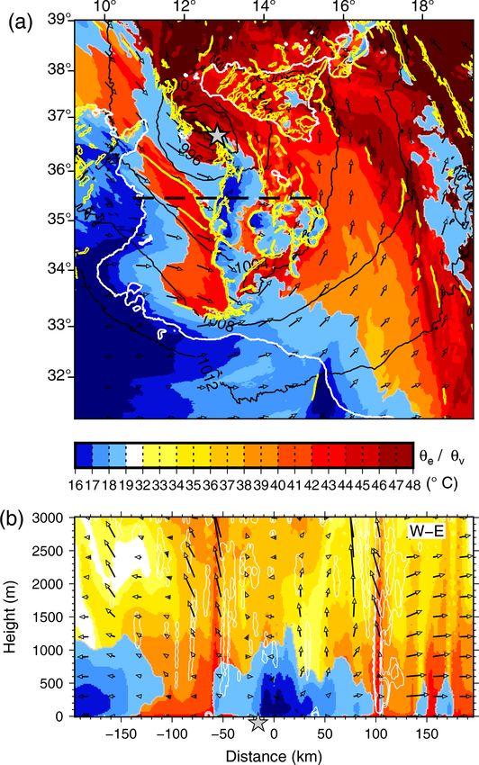
6862                       M.-N. Bouin and C. Lebeaupin Brossier: Surface processes in the 7 November 2014 medicane

Miglietta and Rotunno, 2019). A feature common to many            trolled by surface heat fluxes may be “an important factor of
medicanes is the presence of an elongated upper-level trough      intensification” (Reed et al., 2001, case of January 1982) and
(also know as a PV streamer) bringing cold air with high val-     that the latent heat extraction from the sea is a “key factor of
ues of potential vorticity (PV) from higher-latitude regions.     feeding of the latent-heat release” (Homar et al., 2003, case
Other local effects favouring their development are lee cy-       study of September 1996). Turning off the surface turbulent
clones forming south of the Alps or north of the northern         fluxes during different phases of the cyclone was in contrast
African reliefs (Tibaldi et al., 1990), coastal reliefs favour-   to this view. Indeed, the role of surface enthalpy in feeding
ing deep convection (Moscatello et al., 2008), and relatively     the cyclonic circulation proved important during its earliest
warm sea-surface waters able to feed the process of latent        and mature phases, whereas its role is marginal during the
heat release during their mature phase.                           deepening (Moscatello et al., 2008, case study of Septem-
   The medicane cases meeting all the previous criteria rep-      ber 2006).
resent only a small portion of the Mediterranean cyclones            More recently, studies simulating several cyclones sug-
(e.g. 13 of 200 cases of intense cyclones or roughly one          gested that the impact of the surface fluxes on the cyclone are
per year in the study of Flaounas et al., 2015). Due to this      probably case-dependent (Tous and Romero, 2013; Miglietta
scarcity, clearly defining the properties enabling the separa-    and Rotunno, 2019). The latter work especially compared the
tion of medicanes from other Mediterranean cyclones is still      medicanes of October 1996 (between the Balearic Islands
challenging. A study using dynamical criteria concluded that      and Sardinia) and December 2005 (north of Libya) to investi-
medicanes are very similar to other intense cyclones, with        gate the relative role of the WISHE-like mechanism (WISHE
a slightly weaker upper-level and a stronger low-level PV         – wind-induced surface heat exchange: Emanuel, 1986; Ro-
anomaly (Flaounas et al., 2015). Recent comparative stud-         tunno and Emanuel, 1987) and baroclinic processes. In the
ies (e.g. Akhtar et al., 2014; Miglietta et al., 2017) showed     case of October 1996, the cyclone warm core is formed by
a large diversity of duration, extension (size and vertical ex-   latent heat release fed at the low level by sea-surface heat
tent) and characteristics (dominant role of baroclinic vs. dia-   fluxes. Surface fluxes are above 1500 W m−2 over large areas
batic processes) within the medicane category.                    due to persistent orographic winds bringing cold and dry air
   The role of the large-scale environment like the PV            for several days prior to the cyclone development that con-
streamer and of the associated upper-level jet in medicane        tribute to destabilising the surface layer. The features char-
formation has been the subject of several studies (Reale and      acteristics of tropical cyclones are well marked: warm core
Atlas, 2001; Homar et al., 2003; Flaounas et al., 2015; Carrió    extending up to 400 hPa, symmetry, low-level convergence
et al., 2017). In a case study in September 2006, it was shown    and upper-level divergence, and strong contrast of equivalent
for the first time that the crossing of the upper-level jet by    potential temperature θe (∼ 8 ◦ C) between the surface and
the cyclone resulted in its rapid deepening by interaction be-    900 hPa as evidence of latent heating. Conversely, in the De-
tween low- and upper-level PV anomalies (Chaboureau et al.,       cember 2005 case, the cyclone develops within a large-scale
2012). Recently, the ubiquitous presence of PV streamers and      baroclinic environment, with the PV streamer slowly evolv-
their key role in the development of medicanes have been          ing into a cut-off low. The features similar to tropical cy-
confirmed in several cases (Miglietta et al., 2017). These        clones are less evident: a weaker warm core due to warm-air
studies concluded also that, during their life cycle, medicanes   seclusion and weaker gradient of θe (∼ 3–4 ◦ C) between the
can rely either on purely diabatic processes or on a combina-     surface and 900 hPa. The surface enthalpy fluxes play only
tion of baroclinic and diabatic processes (Mazza et al., 2017;    a marginal role and peak around 1000 W m−2 for a few hours.
Fita and Flaounas, 2018; Miglietta and Rotunno, 2019).            The authors concluded that mechanisms of transition towards
   Conversely, the investigation of the contribution of sur-      medicanes are diverse, especially concerning the role of the
face processes has motivated fewer studies. Some of them          air–sea heat exchanges.
assessed the relative importance of surface heat extraction          As surface fluxes may strongly depend on the SST,
vs. latent heat release and upper-level PV anomaly through-       a change of the oceanic surface conditions may, in theory,
out the cyclone lifetime by using adjoint models or factor        impact the development of a medicane. Several sensitivity
separation techniques (Reed et al., 2001; Homar et al., 2003;     studies investigated the impact of a uniform SST change,
Moscatello et al., 2008; Carrió et al., 2017). They concluded     for instance to anticipate the possible effect of the warm-
that the presence of the upper-level trough during the earlier    ing of Mediterranean surface waters due to climate change.
stage of the cyclone and the latent heat release during its de-   Consistent tendencies were obtained in different case studies
veloping and mature phases are necessary. In contrast, the        (Homar et al., 2003, case of September 1996; Miglietta et al.,
role of surface heat fluxes is more elusive. Like in tropical     2011, case of September 2006; Pytharoulis, 2018, case of
cyclones, the latent heat fluxes always dominate the surface      November 2014; Noyelle et al., 2019, case of October 1996).
enthalpy processes (the sensible heat flux represents 25 % to     As expected, warmer (colder) SSTs lead to more (less) in-
30 % of the turbulent heat fluxes prior to the tropical transi-   tense cyclones even though changes of SST by less than
tion and 15 % to 20 % during the mature phase; Pytharoulis,       ±2 ◦ C result in no significant change in the track, duration
2018). Early studies concluded that low-level instability con-    or intensity of the cyclone.

Atmos. Chem. Phys., 20, 6861–6881, 2020                                             https://doi.org/10.5194/acp-20-6861-2020

M.-N. Bouin and C. Lebeaupin Brossier: Surface processes in the 7 November 2014 medicane                                     6863

   The impact of coupling atmospheric and oceanic models           instability, surface exchanges and latent heat release (Carrió
has been studied mainly using regional climate models on           et al., 2017); or the predictability of the event, depending on
seasonal to interannual timescales. Comparing coupled and          the initial conditions and horizontal resolution of the model
non-coupled simulations showed an impact of the coupling           (Cioni et al., 2018). All those studies showed that the pre-
when the horizontal resolution of the model is at least 0.08◦      dictability of this event and especially of its track is rather
(Akhtar et al., 2014). This resolution is also necessary to re-    low, even with high horizontal (1–2 km) and vertical (50 to
produce, in a realistic way, the characteristic processes of       80 levels) grid resolutions of current operational numerical
medicanes, including warm cores and strong winds at the low        weather prediction (NWP) centres. A recent study based on
level. Coupled simulations resulted in more intense surface        the ensemble forecasts of the ECMWF (European Centre for
heat fluxes, in contrast to what is usually obtained in tropical   Medium-Range Weather Forecasts; Di Muzio et al., 2019)
cyclones due to the strong cooling effect of the cyclone on        showed that the predictability of occurrence (with respect to
the sea surface (Schade and Emanuel, 1999; D’Asaro et al.,         the operational analysis) is good with as early as 7.5 d lead
2007). This can be due to the use of a 1-D ocean model and         time, but the predictability of the position is weak, especially
its limited ability to reproduce the oceanic processes respon-     between 4 and 1 d lead time (their Fig. 6). The predicted cen-
sible for the cooling. The need of higher resolutions to ob-       tral pressure is also consistently 10 to 14 hPa higher than the
serve an impact of the coupling was confirmed by Gaertner          analysed one, whatever the lead time considered.
et al. (2017) and Flaounas et al. (2018). Both studies com-
pared several simulations at the seasonal or interannual scale,    2.1   The 7 November 2014 medicane
both coupled and uncoupled and from several regional cli-
mate modelling platforms. The lack of impact they obtained         On 5 and 6 November 2014, a PV streamer extended
was attributed to the relatively low horizontal resolution of      from northern Europe to northern Africa, bringing cold air
the simulations, between 18 and 50 km. Finally, a case study       (−23 ◦ C) and enhancing instability aloft. A general cyclonic
based on higher-resolution (5 km) simulations of the med-          circulation developed over the Western Mediterranean basin,
icane of November 2011 showed no strong impact of the              while the Eastern Mediterranean was dominated by high
surface coupling. The SST was 0.1 to 0.3 ◦ C lower only,           pressures (Fig. 1a). At the low level on 6 November, the cold
the sea-level pressure (SLP) minimum was 2 hPa higher and          and warm fronts associated with the baroclinic disturbance
the maximum surface wind was 5 m s−1 lower (Ricchi et al.,         were reinforced due to a northward advection of warmer and
2017). The impact of ocean–atmosphere coupling in high-            moist air from northern Africa (Fig. 1b). The system moved
resolution (∼ 1–2 km), convection-resolving models has, to         towards the Strait of Sicily and deepened during the night
the best of our knowledge, not been evaluated yet.                 of 6 to 7 November. In the early hours of 7 November, the
   In the present study, we assess the feedback of the ocean       upper-level PV trough and the low-level cyclone progres-
surface on the atmosphere in the case of the medicane of           sively aligned (Fig. 1c), reinforcing the PV transfer from
November 2014 (also known as Qendresa) using a kilometre-          above and the low-level instability. Strong convection devel-
scale ocean–atmosphere coupled model. We investigate the           oped, with heavy precipitation in the Sicily area. The low-
role of the surface processes, especially during the mature        level system rapidly deepened in the morning of 7 Novem-
phase of the medicane, and we examine the role of the dif-         ber, with a sudden drop of 8 hPa in 6 h, and evolved into
ferent parameters (including SST) controlling these fluxes         the quasi-circular structure of a tropical cyclone, with spi-
throughout the life cycle of the cyclone.                          ral rainbands and a cloudless eye-like centre. The maximum
   A brief description of the medicane, of the modelling tools     intensity was reached at around 12:00 UTC on 7 November
and of the simulation strategy are given in Sect. 2. In Sect. 3,   to the north of Lampedusa (see Fig. 3 for main place names).
the results of the reference simulation are used to describe the   The system drifted eastwards and slowly weakened during
medicane characteristics and life cycle and to present the im-     the afternoon of 7 November, with a first landfall on Malta
pact of the coupling. The roles of the surface conditions and      at around 17:00 UTC. It then moved northeastwards to reach
mechanisms controlling the air–sea fluxes during the differ-       the Sicilian coasts in the evening. It continued its decay dur-
ent phases are assessed in Sect. 4. These results are discussed    ing the following night close to the Sicilian coasts and lost
in Sect. 5, and some conclusions are given.                        its circular shape and tropical-cyclone appearance at around
                                                                   12:00 UTC on 8 November.

                                                                   2.2   Simulations
2   Case study and simulations
                                                                   Three numerical simulations of the event were performed
The case study is the Qendresa medicane that affected the re-      using the state-of-the-art atmospheric model Meso-NH (Lac
gion of Sicily on 7 November 2014. It has been the subject         et al., 2018) and the oceanic model NEMO (Madec and the
of several studies based on simulations. They investigated         NEMO Team, 2016).
the role of SST anomalies or the impact of a uniform SST
change (Pytharoulis, 2018); the respective role of upper-air

https://doi.org/10.5194/acp-20-6861-2020                                            Atmos. Chem. Phys., 20, 6861–6881, 2020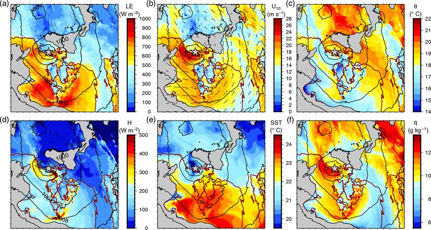
6864                        M.-N. Bouin and C. Lebeaupin Brossier: Surface processes in the 7 November 2014 medicane

Figure 1. Potential vorticity (PV) anomaly at 300 hPa (colour scale) and SLP (isocontours every 4 hPa) at 12:00 UTC on 6 November (a)
and 06:00 UTC on 7 November (c); temperature (colour scale, ◦ C) and wind at 850 hPa at 06:00 UTC on 6 November (b) from the ERA5
reanalysis.

2.2.1   Atmospheric model                                            model shares its physical representation of parameters, in-
                                                                     cluding the surface flux parameterisation, with the French
                                                                     operational model AROME (Seity et al., 2011) used for the
The non-hydrostatic French research model Meso-NH ver-               Météo-France NWP with a current horizontal grid spacing
sion 5.3.0 is used here with a fourth-order centred advec-           of 1.3 km. In this configuration, deep convection is explicitly
tion scheme for the momentum components and the piece-               represented, while shallow convection is parameterised us-
wise parabolic method advection scheme from Colella and              ing the eddy diffusivity Kain–Fritsch scheme (Pergaud et al.,
Woodward (1984) for the other variables, associated with             2009).
a leapfrog time scheme. A C grid in the Arakawa conven-                  In the present study, a first atmosphere-only simulation
tion (Mesinger and Arakawa, 1976) is used for both horizon-          with a grid spacing of 4 km has been performed on a larger
tal and vertical discretisations, with a conformal projection        domain of 3200 km × 2300 km (D1; see Fig. 2). This simula-
system of horizontal coordinates. A fourth-order diffusion           tion started at 18:00 UTC on 6 November and lasted 42 h un-
scheme is applied to the fluctuations of the wind variables,         til 12:00 UTC on 8 November. Its initial and boundary condi-
which are defined as the departures from the large-scale val-        tions come from the ECMWF operational analyses Cy40R1
ues. The turbulence scheme (Cuxart et al., 2000) is based            (horizontal resolution close to 16 km, 137 vertical levels) ev-
on a 1.5-order closure coming from the system of second-             ery 6 h.
order equations for the turbulent moments derived from Re-               As described in the following, this 4 km simulation pro-
delsperger and Sommeria (1986) in a one-dimensional sim-             vides initial and boundary conditions for simulations on
plified form assuming that the horizontal gradients and turbu-       a smaller domain of 900 km × 1280 km (D2; Fig. 2). This do-
lent fluxes are much smaller than their vertical counterparts.       main extension was chosen as a trade-off between computing
The mixing length is parameterised according to Bougeault            time and an extension large enough to represent the physical
and Lacarrere (1989), who related it to the distance that            processes involved in the cyclone life cycle, including the in-
a parcel with a given turbulent kinetic energy at level z            fluence of the coasts. All simulations on the inner domain
can travel downwards or upwards before being stopped by              D2 share a time step of 3 s and their grid (with horizontal
buoyancy effects. Near the surface, these mixing lengths are         grid resolution of 1.33 km and 55 stretched terrain-following
modified according to Redelsperger et al. (2001) to match            levels). Atmospheric and surface parameter fields are issued
both the Monin–Obukhov similarity laws and the free-stream           every 30 min.
model constants. The radiative transfer is computed by solv-
ing long-wave and short-wave radiative transfer models sep-          2.2.2   Oceanic model
arately using the ECMWF operational radiation code (Mor-
crette, 1991). The surface fluxes are computed within the            The ocean model used is NEMO (version 3_6) (Madec and
SURFEX module (Surface Externalisée; Masson et al., 2013)            the NEMO Team, 2016), with physical parameterisations as
using, over sea, the iterative bulk parameterisation ECUME           follows. The total variance dissipation scheme is used for
(Belamari et al., 2005; Belamari and Pirani, 2007) linking           tracer advection in order to conserve energy and enstrophy
the surface turbulent fluxes to the meteorological gradients         (Barnier et al., 2006). The vertical diffusion follows the stan-
through the appropriate transfer coefficients. The Meso-NH           dard turbulent kinetic-energy formulation of NEMO (Blanke

Atmos. Chem. Phys., 20, 6861–6881, 2020                                                https://doi.org/10.5194/acp-20-6861-2020
M.-N. Bouin and C. Lebeaupin Brossier: Surface processes in the 7 November 2014 medicane                                             6865

Figure 2. Map of the large-scale domain D1, with the domain D2 indicated by the solid-line frame and the area of interest (AI) indicated by
the dashed-line frame.

and Delecluse, 1993). In the case of unstable conditions,               2.2.3   Configuration of simulations
a higher diffusivity coefficient of 10 m2 s−1 is applied (Lazar
et al., 1999). The sea-surface height is a prognostic variable          The 3-hourly outputs of the large-scale simulation on D1
solved thanks to the filtered free-surface scheme of Roul-              are used as boundary and initial conditions for three dif-
let and Madec (2000). A no-slip lateral boundary condi-                 ferent simulations on the smaller domain D2, based on
tion is applied, and the bottom friction is parameterised by            the previously described atmospheric and oceanic config-
a quadratic function with a coefficient depending on the 2-D            urations. These three simulations start at 00:00 UTC on
mean tidal energy (Lyard et al., 2006; Beuvier et al., 2012).           7 November and last 36 h, until 12:00 UTC on 8 November.
The diffusion is applied along iso-neutral surfaces for the             The first atmosphere-only simulation called NOCPL uses
tracers using a Laplacian operator with the horizontal eddy             a fixed SST forcing, while the CPL and NOCUR simula-
diffusivity value νh of 30 m2 s−1 . For the dynamics, a bi-             tions are two-way coupled between Meso-NH and NEMO-
Laplacian operator is used with the horizontal viscosity co-            SICIL36. In CPL, the SURFEX–OASIS coupling interface
efficient ηh of −1 × 10⁹ m4 s−1 .                                       (Voldoire et al., 2017) enables exchanging the SST and two-
   The configuration used here is sub-regional and eddy-                dimensional surface currents from NEMO to Meso-NH and
resolving, with a 1/36◦ horizontal resolution over an ORCA              the two components of the momentum flux, the solar and
grid from 2.2 to 2.6 km resolution named SICIL36 (ORCA                  non-solar heat fluxes and the freshwater flux from Meso-NH
is a tripolar grid with variable resolution; Madec and Imbard,          to NEMO every 15 min. The NOCUR run is similar, except
1996), which was extracted from the MED36 configuration                 that the surface currents are not transmitted from NEMO to
domain (Arsouze et al., 2013) and shares the same physical              Meso-NH.
parameterisations with its “sister” configuration WMED36                   In order to ensure that the impact of the coupling in the
(Lebeaupin Brossier et al., 2014; Rainaud et al., 2017). It             NOCUR and CPL configurations originates from the time
uses 50 stretched z levels in the vertical, with level thickness        evolution of the SST rather than from a change in the initial
ranging from 1 m near the surface to 400 m at the sea bottom            SST field, the SST field used as a surface forcing in NOCPL
(i.e. around 4000 m depth) and a partial step representation            is produced by the CPL run, 1 h after the beginning of the
of the bottom topography (Barnier et al., 2006). It has four            simulation (i.e. after the initial adjustment of the oceanic
open boundaries corresponding to those of the D2 domain                 model). This field (Fig. 3) is kept constant throughout the
shown in Fig. 2, and its time step is set to 300 s. The initial         simulation.
and open boundary conditions come from the global 1/12◦
resolution PSY2V4R4 daily analyses from Mercator Océan
International (Lellouche et al., 2013).

https://doi.org/10.5194/acp-20-6861-2020                                                  Atmos. Chem. Phys., 20, 6861–6881, 2020
6866                         M.-N. Bouin and C. Lebeaupin Brossier: Surface processes in the 7 November 2014 medicane

                                                                       the northward shifting of the cyclone occurring in every case
                                                                       in the early hours of 7 November.
                                                                          The deepening and maximum intensity of the simulated
                                                                       cyclone are nevertheless close to the observed ones, even if
                                                                       a direct (i.e. co-localised) comparison is not possible due to
                                                                       the northward shift of its track. A strong deepening of al-
                                                                       most 15 hPa is obtained in the first 12 h of the CPL simulation
                                                                       (Fig. 4b), with a minimum value at 12:30 UTC on 7 Novem-
                                                                       ber close to the minimum observed at Linosa station. This
                                                                       station is the closest point to the best track at the time of the
                                                                       observed maximum intensity of the storm. The surface wind
                                                                       speed peaks at the same time (Fig. 4a), and its time evolu-
                                                                       tion agrees well with METAR observations at the stations of
                                                                       Lampedusa, Pantelleria or Malta. Also, the time evolution of
                                                                       the wind speed averaged over a 50 km radius around the cy-
Figure 3. Comparison of the simulated tracks (triangles) of the non-   clone centre is in good agreement with the control simulation
coupled run (NOCPL; red), coupled run with SST only (NOCUR;            of Cioni et al. (2018). Despite the northward shift of its track,
cyan) and fully coupled run (CPL; blue) with the best track (black
                                                                       the medicane simulated by Meso-NH is very realistic and can
closed circles) based on observations as in Cioni et al. (2018). The
position is shown every hour, with time labels every 3 h, starting
                                                                       be used to explore the processes at play, especially concern-
at 09:00 UTC on 7 November until 12:00 UTC on 8 November. In           ing the role of the sea surface thanks to the CPL simulation.
colours is initial sea surface temperature (SST; ◦ C) at 01:00 UTC
on 7 November.
                                                                       3     Medicane life cycle and coupling impact

                                                                       This part presents first the successive phases of the event
2.3    Validation                                                      based on an analysis of upper-level and mid-troposphere pro-
                                                                       cesses. Then, we assess the impact of accounting for the
Figure 3 compares the tracks of Qendresa obtained in the               short-term evolution of the SST in the atmospheric surface
three different simulations with the best track based on obser-        processes.
vations (brightness temperature from radiance in the 10.8 µm
channel measured by the SEVIRI instrument aboard the                   3.1    Chronology of the simulated event
MSG – Meteosat Second Generation – satellite; see Cioni
et al., 2018). All the simulated tracks are shifted northwards         We use the methodology of Fita and Flaounas (2018) based
with respect to the observations since the beginning of the            on upper-level and low-level dynamics, asymmetry, and ther-
simulations. The mean distance between the simulated and               mal wind to characterise the phases of the medicane. Fig-
observed tracks is close to 85 km, with no significant dif-            ure 5 shows the 300 hPa PV anomaly, SLP, surface wind
ference between the simulations. Cioni et al. (2018) showed            and equivalent potential temperature θe at 850 hPa from the
that using horizontal resolutions finer than 2.5 km is manda-          NOCPL simulation. Phase space diagrams are commonly
tory to accurately represent the fine-scale structure of this cy-      used to describe in a synthetic way the symmetric charac-
clone and its time evolution. Sensitivity studies showed that          teristics of the cyclone as well as the thermal characteristics
better resolution results in simulated track closer to obser-          and extent of its core. The present version in Fig. 6 show-
vations. The best agreement is obtained with a nested con-             ing the evolution of Qendresa from 01:00 UTC on 7 Novem-
figuration and an inner domain at 300 m resolution. In the             ber to 12:00 UTC on 8 November is derived from the orig-
present study, several sensitivity tests were performed on the         inal work of Hart (2003) using the adaptation of Picornell
smaller domain to improve the simulated track: (i) the start-          et al. (2014) for smaller-scale cyclones. The radius used for
ing time of the simulation was changed between 12:00 UTC               computing the low-troposphere thickness asymmetry B and
on 6 November and 00:00 UTC on 7 November with an in-                  the low-troposphere and upper-troposphere thermal winds
crement of 3 h; (ii) the number of vertical levels in Meso-NH          (−VTL and −VTU , respectively) were fitted to the radius
was increased to 100, with stretching to ensure a better sam-          of maximum wind at 850 hPa and is close to 100 km, and
pling in the atmospheric boundary layer; and (iii) the atmo-           the low troposphere and upper troposphere are defined here
spheric simulation was performed without nesting, initial and          as the 925–700 and 700–400 hPa levels, respectively. The
boundary conditions from ECMWF, and a horizontal resolu-               radius value of 100 km is in agreement with several other
tion of 2 km. Note that our inner domain D2 is close in its            studies focusing on medicanes and avoids a smooth-out of
extension to the domain used by Cioni et al. (2018). None              the warm-core structure (Chaboureau et al., 2012; Miglietta
of these tests (eight in total) significantly improved the track,      et al., 2011; Cavicchia et al., 2014; Picornell et al., 2014)

Atmos. Chem. Phys., 20, 6861–6881, 2020                                                  https://doi.org/10.5194/acp-20-6861-2020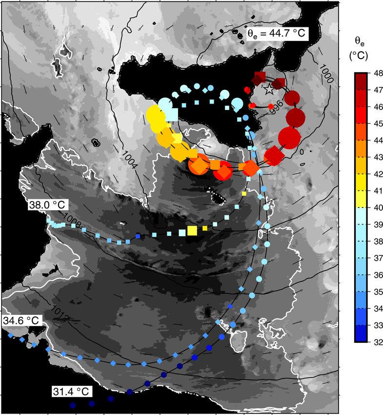
M.-N. Bouin and C. Lebeaupin Brossier: Surface processes in the 7 November 2014 medicane                                              6867

Figure 4. Time series of the maximum of the 10 m wind speed and of the 10 m wind averaged over a 100 km radius around the cyclone
centre (a) and minimum sea-level pressure (b) as obtained in the different simulations on 7 November and 8 November until 12:00 UTC.
The thin red line in (a) indicates the 18 m s−1 wind speed threshold. The background shading (here and in the following time-series plots)
indicates the development (light blue), mature (orange) and decay (grey) phases. The observations of SLP in Linosa (black plain circles) are
shown for comparison in (b); the observations of wind speed from Malta, Lampedusa and Pantelleria are shown in (a) – see text.

but may lead to an underestimation of the cyclone extension.               Then, the upper-level jet moves further over the Ionian Sea
Indeed, the radius of maximum wind is ill defined or larger             and Sicily. The SLP minimum is aligned with the 300 hPa PV
during the first stage of the cyclone, but it is steady and close       anomaly at 11:00 UTC on 7 November (Fig. 5c). This marks
to 90 km during the major part of its lifetime. As a result, the        the beginning of the “mature phase”, with a maximum inten-
diagram obtained is likely less representative of the cyclone           sity at around 12:00 UTC (Fig. 4). The medicane presents
structure during its first hours but fits well after 10:00 UTC.         the circular shape typical of tropical cyclones with spiral
   At 06:00 UTC on 7 November, the PV streamer has moved                rainbands, and a warm, symmetric core (Fig. 5d) extended
northwards from Libya and is located to the south of the                up to 400 hPa (Fig. 6). The upper-level PV anomaly stays
SLP minimum (Fig. 5a). A south–north cold front is visible              wrapped around the SLP until 17:00 UTC, and both struc-
in the 850 hPa θe , east of the cyclone centre, and the medi-           tures drift eastwards to the south of Italy (Fig. 5e). The medi-
cane centre is located under the left exit of the upper-level jet       cane slowly decreases in intensity (Fig. 4) until it makes land-
(Fig. 5b). The minimum SLP starts to decrease until reach-              fall in the southeast of Sicily at 18:00 UTC. The cold front
ing 985 hPa at around 11:00 UTC, corresponding to a strong              drifts eastwards away of the cyclone centre, evolving into an
deepening rate of 1.4 hPa h−1 for 10 h. This phase also marks           occluded front wrapped around the SLP minimum (Fig. 5f).
the increase in the maximum wind at the low level and in                This mature phase, although the most intense of the cyclone,
the wind speed averaged over a 100 km radius around the cy-             produces more scattered rainfall than the development phase
clone centre (Fig. 4). It is referred to as “development phase”         (Fig. 7).
in the following. The heaviest rainfall occurs here (Fig. 7),              The cyclone then moves northeastwards towards the Io-
with 10 h accumulated rain above 200 mm locally and instan-             nian Sea and continuously weakens until 12:00 UTC on
taneous values above 50 mm h−1 east of Sicily and at sea be-            8 November (“decay phase” hereafter). The SLP minimum
tween Pantelleria and Malta. As in Fita and Flaounas (2018),            steadily increases (Fig. 4); at this point, the upper-level PV
the maximum thermal wind is obtained during this phase                  anomaly has evolved into a cut-off and is still aligned with
(Fig. 6).                                                               the cyclone centre (Fig. 5g), and the 850 hPa warm core has
                                                                        extended ∼ 250 km around the cyclone centre (Fig. 5h).

https://doi.org/10.5194/acp-20-6861-2020                                                   Atmos. Chem. Phys., 20, 6861–6881, 2020
6868                         M.-N. Bouin and C. Lebeaupin Brossier: Surface processes in the 7 November 2014 medicane

                                                                       3.2   SST evolution

                                                                       Taking into account the effect of the SST change only
                                                                       (NOCUR) results in a slightly slower and weaker deepen-
                                                                       ing by 1.5 hPa and a maximum wind speed that is 3 m s−1
                                                                       higher (Fig. 4). Including the effect of the surface currents
                                                                       on the atmospheric boundary layer gives a slightly more in-
                                                                       tense cyclone (1.5 hPa less and 8 m s−1 stronger maximum
                                                                       wind). Figure 3 shows no significant difference in the tracks
                                                                       between the NOCPL, NOCUR and CPL simulations, except
                                                                       when the cyclone centre loops east of Sicily at the end of the
                                                                       day. The median values of the SST difference between CPL
                                                                       and NOCPL over the whole domain and the values of the
                                                                       5 %, 25 %, 75 % and 95 % quantiles are shown in Fig. 8. The
                                                                       median surface cooling is very weak (0.1 ◦ C at the end of the
                                                                       development phase, ∼ 0.2 ◦ C at the beginning of the decay
                                                                       phase). Its evolution during the decay phase is also weak,
                                                                       with values of 0.25 ◦ C at 23:00 UTC, on 7 November. The
                                                                       maximum cooling is 0.6 ◦ C. To focus on the effects of this
                                                                       surface cooling on the surface processes feeding the cyclone,
                                                                       we used a conditional sampling technique to isolate the ar-
                                                                       eas with enthalpy flux above 600 W m−2 (this corresponds to
                                                                       the mean value of the 80 % quantile of the enthalpy flux on
                                                                       the day of 7 November). The enthalpy flux is defined here as
                                                                       the sum of the latent heat flux LE and the sensible heat flux
                                                                       H . In this area (EF600 hereafter), the SST difference and its
                                                                       time evolution are slightly larger, with a median difference
                                                                       of −0.2 ◦ C at the beginning of the mature phase and −0.4 ◦ C
                                                                       at the end of 7 November. In NOCUR, the SST difference in
                                                                       EF600 is slightly larger than in CPL, but the difference is not
                                                                       significant. The SST cooling in this area of less than 0.4 ◦ C
                                                                       (median value) is much weaker than typical cooling values
                                                                       observed under tropical cyclones, which commonly reach 3
                                                                       to 4 ◦ C (e.g. Black and Dickey, 2008). In addition, the spa-
                                                                       tial extent of the cooling does not form a wake as in tropical
                                                                       cyclones (not shown).
                                                                          The conclusion of this part is that surface cooling is 1 or-
                                                                       der of magnitude smaller than what is obtained under trop-
                                                                       ical cyclone, with no significant impact of the surface cur-
                                                                       rents. However, quantifying the surface cooling in other med-
Figure 5. Potential vorticity at 300 hPa (colour scale) and SLP
(isocontours every 4 hPa; the 1000 hPa isobar is in bold) (a, c, e,
                                                                       icanes could lead to contrasting results. For instance, a sur-
g) and equivalent potential temperature (◦ C; colour scale) and wind   face cooling of 2 ◦ C was obtained in an ocean–atmosphere–
at 850 hPa, SLP, and 6 PVU at 300 hPa isocontours (red) (b, d, f,      waves coupled simulation of a strong storm in the Gulf of
h) from the NOCPL simulation.                                          Lion (Renault et al., 2012). Investigating the reasons of such
                                                                       a discrepancy are beyond the scope of the present work. The
                                                                       stronger cooling could be due to the storm track staying at the
   In the following, the impact of the ocean–atmosphere cou-           same place in the Gulf of Lion for a long time. The difference
pling on the cyclone intensity is assessed by comparing the            can also come from a different oceanic preconditioning (their
results of the CPL, NOCUR and NOCPL simulations. The                   case occurred in May), with stronger stratification or a shal-
time period for this comparison is 7 November only, as the             lower mixed layer that amplifies cooling due to the mixing
medicane lost a large part of its intensity in the evening of          and entrainment process.
7 November.

Atmos. Chem. Phys., 20, 6861–6881, 2020                                                 https://doi.org/10.5194/acp-20-6861-2020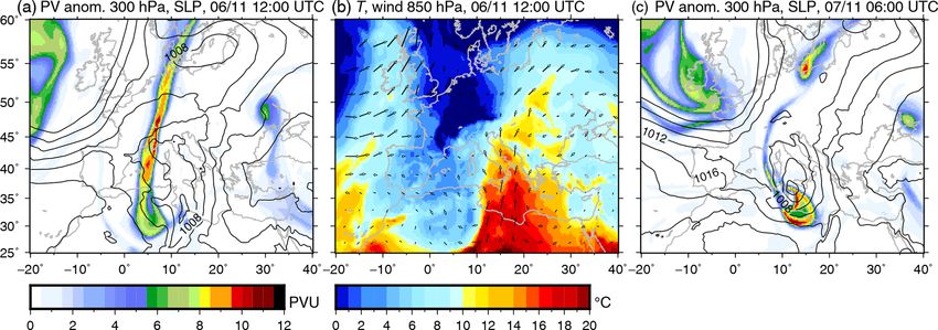
M.-N. Bouin and C. Lebeaupin Brossier: Surface processes in the 7 November 2014 medicane                                            6869

Figure 6. Phase diagram of the NOCPL-simulated cyclone from 01:00 UTC on 7 November to 12:00 UTC on 8 November, with low-
tropospheric thickness asymmetry inside the cyclone (B) with respect to low-tropospheric thermal wind (−VLT ) (a) and upper-tropospheric
thermal wind (−VUT ) with respect to low-tropospheric thermal wind (b). The development phase is in blue, the mature phase in red and the
decay phase in black.

Figure 7. Histogram of the mean rain rate distribution (in number of   Figure 8. Time series of the median differences between the SST in
grid points) for the development (blue) and mature (red) phases in     the CPL and NOCPL simulations, in the whole domain (red) and in
the NOCPL simulation. The enclosed figure zooms in on the highest      the EF600 area (blue; see text for definition), on 7 November. The
rates.                                                                 boxes indicate the 25 % and 75 % quantiles and the whiskers the 5 %
                                                                       and 95 % quantiles. The SST differences in the EF600 area between
                                                                       the NOCUR and NOCPL simulations are also shown (cyan). Some
3.3   Impact on turbulent surface exchanges                            of the boxes have been slightly shifted horizontally for clarity.

A comparison of the time evolution of the turbulent fluxes
in the NOCPL and CPL simulations shows very weak dif-                     In the following, except if otherwise specified, the results
ferences even in the EF600 area (Fig. 9a). At the end of the           of the NOCPL simulation are used to investigate the medi-
run, the mean difference of the enthalpy flux is 25 W m−2 ,            cane behaviour, focusing on the area of interest (AI in Fig. 2).
with a standard deviation of 13 W m−2 . This is weak com-
pared to the values of the turbulent fluxes on this area, be-
tween 500 and 800 W m−2 for LE and 100 and 250 W m−2                   4   Role of surface fluxes and mechanisms
for H . Expressed in percentage of the fluxes, the relative
difference is ∼ 2 % at the beginning of the mature phase               This section investigates which surface parameters control
and 5 % at 21:00 UTC on 7 November. The difference of H                the surface heat fluxes during the different phases of the med-
is 7 ± 4 W m−2 (relative difference between 4 % and 10 %).             icane, among the SST, surface wind, temperature and humid-
Thus, coupling has a very weak impact on the turbulent heat            ity.
fluxes even in the EF600 area. Again, the effect of the surface
currents (CPL vs. NOCUR in Fig. 9b) is not significant.

https://doi.org/10.5194/acp-20-6861-2020                                                 Atmos. Chem. Phys., 20, 6861–6881, 2020
6870                               M.-N. Bouin and C. Lebeaupin Brossier: Surface processes in the 7 November 2014 medicane

Figure 9. Time series of the mean values and standard deviations (error bars) of the total turbulent heat flux (blue), latent heat flux (cyan)
and sensible heat flux (red) in the CPL (open circles) and NOCPL (triangles) simulations (a) and of the mean difference between CPL and
NOCPL turbulent fluxes (open circles; same colour code) and between NOCUR and NOCPL turbulent fluxes, in percentage relative to the
NOCPL values (b) in the EF600 area.

4.1     Representation of surface fluxes and methods                     and Cen the neutral transfer coefficient for heat and mois-
                                                                         ture, and L the Obukhov length (which depends, in turn, on
In numerical atmospheric models, the turbulent heat fluxes               the virtual potential temperature at the first level and on the
are classically computed as a function of surface parameters             friction velocity u∗ ). In the ECUME parameterisation used
using bulk formulae:                                                     in this study, the neutral transfer coefficients Chn and Cen
                                                                         are defined as polynomial functions of the 10 m equivalent
H = ρcp Ch 1U 1θ,                                               (1)      neutral wind speed (defined as in Geernaert and Katsaros,
LE = ρLv Ce 1U 1q.                                              (2)      1986). They also depend on the wind speed at 10 m and
                                                                         on the Obukhov length through the stability functions. The
Here, ρ is the air density, cp the air thermal capacity and Lv           Obukhov length is expressed as in Liu et al. (1979):
the vaporisation heat constant. The gradient 1U corresponds
to the wind speed at the first level with respect to the sea sur-                Tv2 u2∗
face, 1θ is the difference between the SST and the potential             L=−             ,                                                (5)
                                                                                 κgTv∗
temperature at the first level θ , and 1q is the difference be-
tween the specific humidity at saturation, with temperature              with Tv being the virtual temperature at the first level, de-
equal to SST and the specific humidity at the first level. The           pending on the temperature and specific humidity, and Tv∗
transfer coefficients Ch and Ce are defined as                           the scale parameter for virtual temperature, depending on
                        1/2                                              the temperature and humidity at the first level. As a conse-
  1/2              Chn                                                   quence, the transfer coefficients depend as the fluxes on the
Ch      =         1/2
                                   ,                            (3)
            1−
                 Chn
                        ψT (z/L)                                         wind speed, on the temperature and specific humidity at the
                  κ
                                                                         first level, and on the SST. In the following, we do not distin-
and                                                                      guish between the temperature and potential temperature at
                        1/2                                              the first level.
  1/2              Cen                                                      The time evolution of the median values and 5 %, 25 %,
Ce      =         1/2
                               ,                                (4)
            1 − Cen                                                      75 % and 95 % quantiles of the latent and sensible heat fluxes
                 κ ψq (z/L)
                                                                         is given in Fig. 10a for 7 November, in the EF600 area, and
with κ being the von Karman’s constant, ψT and ψq em-                    the time evolution of the median values and quantiles of the
pirical functions describing the stability dependence, Chn               SST in Fig. 10b. The latent heat flux is always much higher

Atmos. Chem. Phys., 20, 6861–6881, 2020                                                      https://doi.org/10.5194/acp-20-6861-2020
M.-N. Bouin and C. Lebeaupin Brossier: Surface processes in the 7 November 2014 medicane 6871
Table 1. Spearman’s rank correlations between the enthalpy flux,
latent and sensible heat flux, and related parameters (10 m wind
speed U10 , potential temperature at 10 m θ, SST and humidity at
10 m q) at 09:00 UTC on 7 November, from the CPL simulation, in
the EF600 area.
U10 θ SST q
H + LE 0.66 −0.20 0.35 0.48
LE 0.65 0.10 0.36 0.33
H 0.38 −0.70 0.21
U10 −0.10 −0.25 0.84
θ −0.04 −0.03
SST −0.18
Table 2. Same as Table 1 but at 13:00 UTC on 7 November.
Figure 10. Time series of the median values of latent (blue) and U10 θ SST q
sensible heat fluxes (red; a) and of SST (b) in the EF600 area (see H + LE 0.62 −0.14 0.28 0.49
text) in the NOCPL run on 7 November. The boxes corresponds to LE 0.49 0.22 0.42 0.23
the 25 % and 75 % quantiles and the whiskers to the 5 % and 95 % H 0.55 −0.72 −0.10
quantiles. U10 −0.19 −0.38 0.87
θ 0.41 −0.32
SST −0.34
than the sensible heat flux, as this is generally the case at sea
when the SST is above 15 ◦ C (e.g. Reale and Atlas, 2001).
The sensible heat flux represents here 22 % of the enthalpy Table 3. Same as Table 1 but at 18:00 UTC on 7 November.
flux during the development phase and 12 % to 15 % dur-
ing the decay phase. Both fluxes have asymmetric distribu- U10 θ SST q
tions, with upper tails (95 %) longer than lower tails (5 %). H + LE 0.31 −0.09 0.32 0.17
This is partly due to the conditional sampling (LE + H > LE 0.16 0.26 0.46 −0.03
600 W m−2 ) used here, as low fluxes are cut off. The median H 0.37 −0.75 −0.20
value of H is maximum at the end of the development phase U10 −0.02 −0.52 0.93
(180 W m−2 at 08:00 UTC), while its 95 % quantile is maxi- θ 0.40 −0.04
mum at the beginning of the development phase (332 W m−2 SST −0.49
at 04:00 UTC). During the mature phase, both the median
and 95 % quantile values of H decrease continuously. Con-
versely, the median value of LE is maximum (635 W m−2 ) we used the rank correlation of Spearman, which corre-
at 09:00 UTC during the development phase, and it stays ap- sponds to the linear correlation between the rank of the
proximately constant until 15:00 UTC. The 95 % quantile is two variables in their respective sampling (Myers et al.,
maximum (845 W m−2 ) at the end of the development phase. 2010). This metric enables relating the variables of interest
LE starts to decrease later and more slowly than H (at around monotonically rather than linearly and is more appropriate
15:00 UTC, as the system has started to weaken). The median in the case of non-linear relationships.
values of LE in this EF600 sampling are constant or slightly The co-variabilities are analysed in the whole domain first,
increasing until the evening (20:00 UTC), whereas the min- to determine the main contribution to the fluxes globally, then
imum values (5 % quantile) increase continuously until the in the EF600 area to isolate surface processes controlling the
end of the day. Again, this is probably partly due to the sam- growth and maturity of the medicane. The values are given
pling used here. in Tables 1 to 3 for the EF600 area and for three time periods
The distributions of the SST are asymmetric throughout of the development, mature and decay phases, respectively,
the event, with lower tails much longer than upper tails i.e. 09:00, 13:00 and 18:00 UTC on 7 November.
(Fig. 10b). The SST maximum (close to 24 ◦ C) is almost con-
stant with time. The lower and median values vary due to the 4.2 Development phase
conditional sampling EF600 and the motion of the cyclone
away from the warm SST area. At the low level, this phase corresponds to a low-pressure
To investigate the mutual dependencies and co- system resulting from the evolution of the instability gener-
variabilities of the fluxes and parameters listed above, ated by the lee cyclone of the northern African relief, with
https://doi.org/10.5194/acp-20-6861-2020 Atmos. Chem. Phys., 20, 6861–6881, 20206872 M.-N. Bouin and C. Lebeaupin Brossier: Surface processes in the 7 November 2014 medicane
Figure 12. Time series of Spearman’s rank-order correlation rs be-
tween the latent heat flux LE and 10 m wind speed (green), potential
temperature at 10 m (red), SST (blue), and specific humidity at 2 m
(cyan) in the whole domain (a) and in the EF600 area (b) in the CPL
simulation.
limit of 19 ◦ C for θv – Ducrocq et al., 2008; Bresson et al.,
2012). Some of these cold pools result from evaporation un-
der convective precipitation, while those located at sea along
the northern African coast originate from dry and cold air
advected from inland. The discrimination between these two
kinds of cold pools was done using a simulation without the
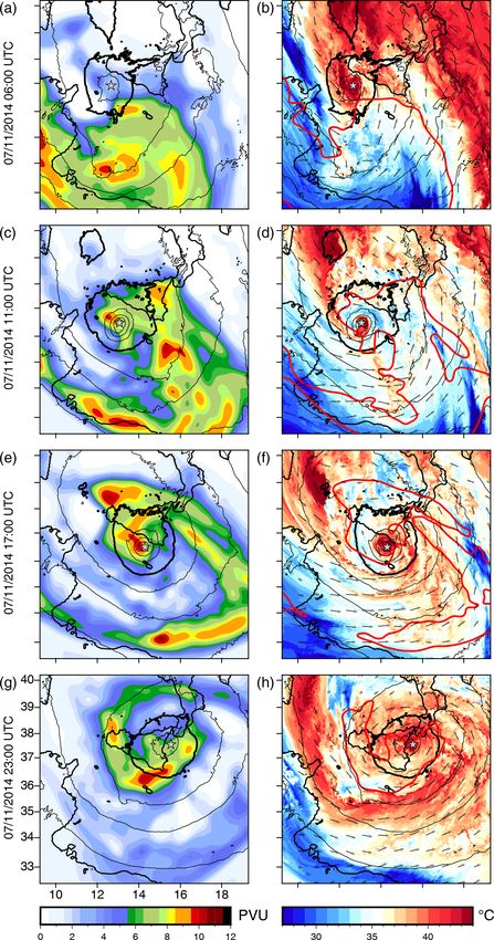
Figure 11. Map of equivalent potential temperature (warm colours) latent heat transfer due to rain evaporation (not shown here).
and virtual potential temperature below 19 ◦ C (blue shades) at first The cold and moist air spreads to the surface, following den-
level; horizontal convergence rate above 1 × 10⁻³ m s−2 at 100 m sity currents, and is advected northeastwards by the low-level
(yellow contours), 10 m wind (arrows) and SLP (black contours) at flow. To the west and south of the domain, cold pools were
08:30 UTC on 7 November (a); and vertical cross section of equiva- formed at night by radiative processes over land and were
lent potential temperature and virtual potential temperature (colour advected over sea with a vertical extent of ∼ 1000 m (see the
scale), tangential wind (black vectors; the vertical component is am- westernmost part of the W–E transect; Fig. 11b).
plified by a factor 20), and potential vorticity anomaly (white con- The upwind edge of the cold pools is the place of strong
tour at 5 PVU) along a west–east transect (b) (dashed line in a).
horizontal convergence at the low level, leading to uplift and
Grey stars indicate the position of the SLP minimum.
deep convection of air masses with high θe . During the de-
velopment phase, the cold pools move northwards with the
southerly flow, towards the centre of the cyclone. Then, they
strong baroclinic structures. During the first hours, the ar- contribute to triggering convection in the northwesterly low-
eas of heavy precipitation are co-localised with frontal struc- level flow with high θe (Fig. 11b). The warm surface anomaly
tures. A warm sector is visible east of the domain, with a cold propagates close to the cyclone centre (now located under the
front extending southeast from the south of Italy and a very 300 hPa PV anomaly) up to 3000 m and generates a low- to
strong low-level convergence between the southeasterly flow mid-troposphere PV anomaly. At the same time, a dry-air in-
in the warm sector and the south-to-southwesterly flow in the trusion from the upper levels brings air masses with low θe
cold sector (see Fig. 5b). and relative humidity below 20 % to 3000 m, resulting in an
At 08:30 UTC on 7 November (Fig. 11), strong conver- upper-to-mid-troposphere PV anomaly (Fig. 15a and c).
gence lines develop close to the cyclonic centre, between To identify the surface parameters controlling evaporation
Sicily and Tunisia. The low-level virtual potential temper- at sea, the time evolution of the Spearman’s rank correlations
ature θv superimposed onto the equivalent potential tempera- between LE, U10 , θ , the SST and q is given in Fig. 12 and
ture θe is used here as a marker of cold pools (with an upper Tables 1 to 3.
Atmos. Chem. Phys., 20, 6861–6881, 2020 https://doi.org/10.5194/acp-20-6861-2020M.-N. Bouin and C. Lebeaupin Brossier: Surface processes in the 7 November 2014 medicane 6873
Figure 13. Maps of the turbulent heat fluxes LE (a), H (d), 10 m wind U10 (b), 10 m potential temperature (c), SST (e) and specific humidity
at 2 m (f) at 09:00 UTC on 7 November in the CPL simulation.
During this phase, in the whole domain, the parameters
governing LE are the SST and the wind (positively corre-
lated), the specific humidity (negatively) and the potential
temperature (negatively). Potential temperature and humid-
ity are also strongly positively correlated (rs = 0.55 over the
whole domain) because cold and dry air is advected from
the Tunisian and Libyan continental surface by the southerly
low-level flow (Fig. 13b, c and f; at 09:00 UTC). This air
mass progressively charges itself in heat and moisture in the
area of strongest enthalpy fluxes at sea to the north of Libya
(Fig. 13a). The EF600 area, with strong fluxes and cold and
dry air, corresponds also to warm SSTs (Fig. 13e). Here, LE
is mainly controlled by the wind and by the SST, θ has no
effect (weak or negative correlations; Fig. 12b, Table 1) and
q has a weak effect.
LE is always much higher than H (Fig. 10a), resulting in
the “strong flux area” EF600 being controlled by LE rather
than H . LE is also more homogeneous than H in EF600.
However, H can be strong locally (Fig. 13d). During this
Figure 14. Same as Fig. 12 but between the sensible heat flux H
development phase, H is controlled mainly by θ at the first and 10 m wind speed (green), potential temperature at 10 m (red),
level (Fig. 14), partly indirectly through the stratification and and SST (blue).
transfer coefficient (not shown). In the EF600 area also, H is
mainly governed by θ (rs = −0.70 at 09:00 UTC), the SST
influence is always weak and the wind plays a secondary
role. The enhanced control by the potential temperature is 4.3 Mature phase
partly due to the continental air masses advected from north-
ern Africa and partly to the presence of the cold pools under At 13:00 on 7 November, the PV anomalies at 700 and
the areas of deep convection and strong wind. 300 hPa are aligned (Fig. 15c, e). A zonal cross section on
the SLP minimum shows that a low-level PV anomaly above
https://doi.org/10.5194/acp-20-6861-2020 Atmos. Chem. Phys., 20, 6861–6881, 20206874 M.-N. Bouin and C. Lebeaupin Brossier: Surface processes in the 7 November 2014 medicane
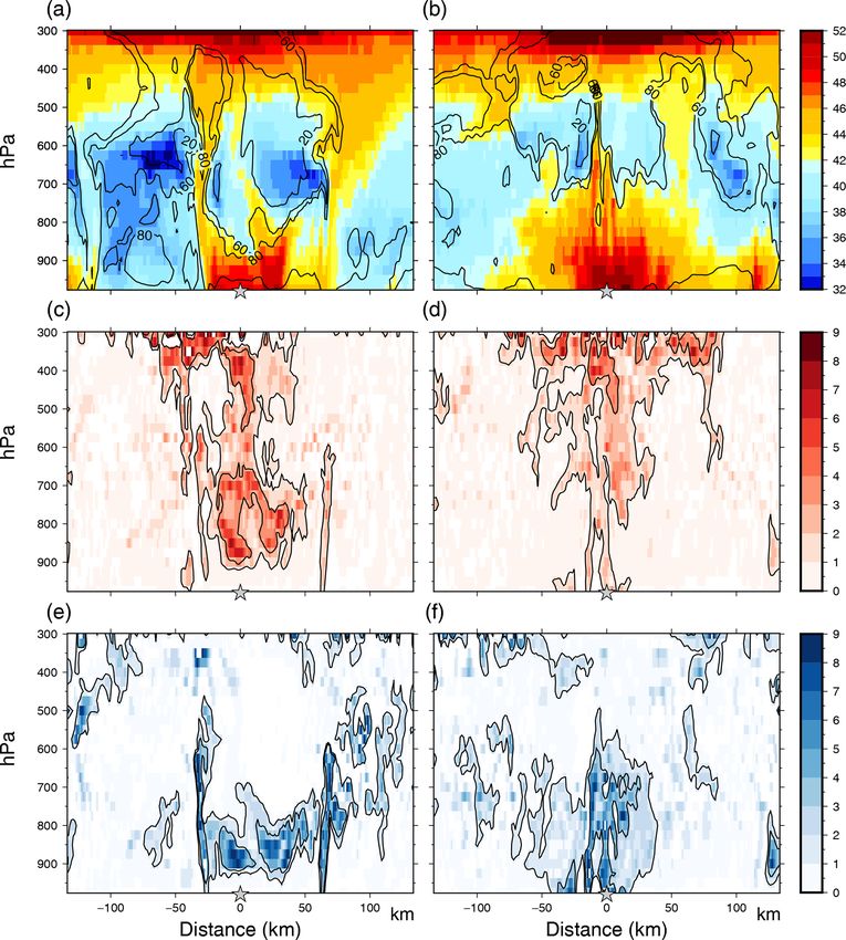
Figure 15. Vertical cross sections of equivalent potential temperature θe (◦ C; colour scale) and relative humidity (%; isolines) (a, b), DPV
(intensity) (c, d), and WPV (intensity) (e, f) on a west–east transect across the cyclone centre, at 13:00 (a, c, e) and 18:00 UTC (b, d, f) on
7 November, in the CPL simulation. The black contours in (c) to (f) correspond to intensities 1 and 3 (as defined in Miglietta et al., 2017).
5 PVU formed around the cyclone centre, extending from the influence of the humidity (Fig. 12, Table 2). The EF600 area
surface up to the 300 hPa anomaly (Fig. 15). The warm core extends further north, closer to the cyclone centre, away from
extends up to 850 hPa (Fig. 15a). Its upward development is the area of cold and dry low-level air. This cold-air inflow
limited by colder air (low θe ) brought from aloft. There is starts to warm and moisten under the combined impact of
low-level convergence (up to 800 hPa) towards the cyclone the diurnal warming of the continental surfaces (not shown)
centre, and deep convection close to the centre, but no or and of the strong enthalpy fluxes offshore (Fig. 16a, c and f).
very weak divergence at the mid-troposphere to upper tro- The sensible heat flux is still controlled by the temperature,
posphere. The cyclonic circulation was reinforced with hor- with an increasing influence of the wind (Table 2).
izontal wind speed above 8 m s−1 at every level more than
10 km away from the cyclone centre. 4.4 Decay phase
During this phase and the previous one, over the whole do-
main as in the EF600 area, evaporation is controlled equiv- In the afternoon of 7 November, the cyclone first moves to-
alently by the SST and the wind speed, with a decreasing wards colder SSTs in the east of the Strait of Sicily (Fig. 3).
Then, it crosses Sicily and reaches the Ionian Sea with even
Atmos. Chem. Phys., 20, 6861–6881, 2020 https://doi.org/10.5194/acp-20-6861-2020M.-N. Bouin and C. Lebeaupin Brossier: Surface processes in the 7 November 2014 medicane 6875 Figure 16. Same as Fig. 13 but at 13:00 UTC on 7 November. colder SSTs at around 20:00 UTC before slowly decaying During the decay phase and in the whole domain the in- and losing its tropical characteristics. Back trajectories are fluence of the humidity on LE is weak (Fig. 12a). EF600 is used to check whether warm- and moist-air extraction from still located on warm SSTs south of the domain (Fig. 18a, the sea surface contributes to high θe values obtained around e) and corresponds also to the strongest winds on the right- the cyclone centre. They are based on the method of Schär hand side of the cyclone (Fig. 18b). Within this area, there and Wernli (1993), adapted by Gheusi and Stein (2005). The is almost no influence of the temperature or humidity on LE chosen trajectories originate from three different places and (Table 3). The influence of the wind speed is decreasing; the arrive at the same place, at three vertical levels surrounding role of the SST is strong until 21:00 UTC. After that, the the level closest to 1500 m, at 23:00 UTC on 7 November cyclone reaches the northern Ionian Sea with much colder (Fig. 17). Their equivalent potential temperature ranges from SSTs, and the effect of the wind speed becomes dominant at 31 to 38 ◦ C at their first appearance in the domain and is close the very end (Fig. 12b). The sensible heat flux is governed to 45 ◦ C on average at their final point. Of these trajectories, by the wind (see the strong N–S gradient in Fig. 18b) rather θe increases almost continuously, with a strong jump during than by the low-level temperature, except in the northern part their transit at the low level (below 500 m) above the sea in of EF600 (where the wind speed is also the highest). the EF600 area (white contour in Fig. 17). A separate anal- In summary, at the scale of the domain, both strong winds ysis of the two different stages in the trajectories was per- (in the cold sector during the development phase, then close formed. Stage 1 corresponds to the period when the particles to the cyclone centre and on its right side) and warm SSTs remain in the low-level flow (between 200 and 1200 m a.s.l.) (in the south of the domain) are necessary for strong la- south and east of Sicily and stage 2 to their convective ascent tent heat fluxes. Within the area of strong fluxes (also strong from ∼ 300 to 1500 m. During stage 1, the potential tem- winds and warm SSTs), the evaporation is mainly controlled perature of the particles decreases by 1 ◦ C on average, while by the wind (development and mature phases) instead of by the mixing ratio increases by 2.8 g kg−1 . This shows that the the SST (decay phase). In contrast, the sensible heat flux increase in θe is due to strong surface evaporation. During depends mainly on the potential temperature in the surface stage 2, the mixed ratio of the particles decreases by 2 g kg−1 , layer. Colder air masses lead to strong sensible heat flux and their potential temperature increases by 4.1 ◦ C. This in- rather than strong wind or warmer SSTs. During the two first dicates condensation and latent heating and demonstrates the phases, cold air is either advected from northern Africa or strong role of the sea surface in increasing the moisture and created by evaporation under convective precipitation (cold heat of the low-level flow before its approach on the cyclone pools). During the decay phase, strong latent heat transfer centre and of diabatic processes in reinforcing its warm core. https://doi.org/10.5194/acp-20-6861-2020 Atmos. Chem. Phys., 20, 6861–6881, 2020
You can also read