Flood depth estimation by means of high-resolution SAR images and lidar data - NHESS
←
→
Page content transcription
If your browser does not render page correctly, please read the page content below

Nat. Hazards Earth Syst. Sci., 18, 3063–3084, 2018
https://doi.org/10.5194/nhess-18-3063-2018
© Author(s) 2018. This work is distributed under
the Creative Commons Attribution 4.0 License.

Flood depth estimation by means of high-resolution
SAR images and lidar data
Fabio Cian1 , Mattia Marconcini2 , Pietro Ceccato3 , and Carlo Giupponi1
1 Department   of Economics, University of Venice Ca’ Foscari, Venice, 30121, Italy
2 DFD   German Aerospace Center (DFD-DLR), 82234 Weßling, Germany
3 International Research Institute for Climate and Society (IRI), Columbia University, New York, USA

Correspondence: Fabio Cian (fabio.cian@unive.it)

Received: 29 May 2018 – Discussion started: 29 June 2018
Revised: 19 October 2018 – Accepted: 6 November 2018 – Published: 19 November 2018

Abstract. When floods hit inhabited areas, great losses are       ability of these events to happen is also exacerbated by land-
usually registered in terms of both impacts on people (i.e.,      use change and in particular, by settlement growth, which
fatalities and injuries) and economic impacts on urban areas,     increases soil sealing and hence water runoff. The ultimate
commercial and productive sites, infrastructures, and agricul-    consequence would be an increase in fatalities and injuries,
ture. To properly assess these, several parameters are needed,    but also in economic losses in urban areas, commercial and
among which flood depth is one of the most important as it        productive sites, infrastructures, and agriculture.
governs the models used to compute damages in economic               Flood risk and impacts are not sufficiently understood and
terms. This paper presents a simple yet effective semiauto-       documented and need to be monitored systematically with
matic approach for deriving very precise inundation depth.        improved precision as underlined by the European Union
First, precise flood extent is derived employing a change de-     Floods Directive (European Commission, 2007). This is par-
tection approach based on the normalized difference flood in-     ticularly important to support climate change adaptation poli-
dex computed from high-resolution synthetic aperture radar        cies as well as to develop robust public disaster relief funds,
imagery. Second, by means of a high-resolution lidar digital      risk profiles for financial institutes, risk portfolios for rein-
elevation model, water surface elevation is estimated through     surance companies, and profiles of risk in supply chain for
a statistical analysis of terrain elevation along the boundary    multinational companies (Mysiak, 2013; Desai et al., 2015).
lines of the identified flooded areas. Experimental results and   In order to assess flood impacts, in addition to their extent,
quality assessment are given for the flood that occurred in the   several other parameters, such as flow velocity, debris factor,
Veneto region, northeastern Italy, in 2010. In particular, the    and inundation depth, shall be monitored during the event.
method proved fast and robust and, compared to hydrody-           Here, flood depth is particularly important since it governs
namic models, it requires sensibly less input information.        the damage functions (or vulnerability curves or loss func-
                                                                  tions), which define the expected loss given a certain flood
                                                                  depth (Mojtahed, 2013; Scorzini, 2017).
                                                                     Therefore, in ex post assessment deriving flood depth is
1   Introduction                                                  essential to quantify impacts and damages, to better char-
                                                                  acterize flood risk, and to implement disaster risk reduction
Climate science foresees a future in which extreme weather        measures. Furthermore, it also has a key role in supporting
events could happen with increased frequency and strength         emergency response, assessing accessibility and designing
as a consequence of anthropogenic activities. Specifically,       suitable intervention plans, calculating water volumes, allo-
climate change would favor extreme precipitations, which          cating resources for water pumping, and rapidly estimating
could cause riverine, flash, and coastal floods (i.e., the main   the costs for intervention and reconstruction.
source of losses in the world as reported by NatCatSER-
VICE, 2015) to occur more and more often. The higher prob-

Published by Copernicus Publications on behalf of the European Geosciences Union.
3064                        F. Cian et al.: Flood depth estimation by means of high-resolution SAR images and lidar data

   In Veneto, northeastern Italy, several floods caused ma-        of permanent water bodies (mostly characterized by low and
jor damage in the past decade, for example the one that oc-        stable backscattering values) from temporary water surfaces;
curred in 2010 in the city of Vicenza and its surroundings,        on the other hand, it might occur that land-cover changes as-
which was the most serious in the area over the last 50 years      sociated with different backscattering values at the two con-
(ARPAV, 2010). Moreover, extreme weather events are ex-            sidered time steps (as typically occurs for crops) can lead
pected to increase in the future due to climate change (Zollo      to overestimation of flooded areas (Giustarini, 2013, 2015;
et al., 2015) in the entire region, and thus there is a great      Long, 2014; Matgen, 2007).
interest in monitoring floods.                                        The abovementioned approaches generally fail to detect
   To this purpose, remote sensing and in particular syn-          floods occurring in vegetated areas where the water surface
thetic aperture radar (SAR) data have been playing an im-          is obscured by tree branches and leaves. This might become
portant role for decades, allowing, during crises, the deriva-     a critical issue in regions characterized by a large amount of
tion of flood extent maps like those provided by the Euro-         woodland and medium to tall vegetation and requires users
pean Copernicus Emergency Management Service (Coper-               to be extra vigilant to interpret the results. Furthermore, due
nicus EMS) or the International Charter on Space and Ma-           to lack of details in medium-/low-resolution SAR data and to
jor Disaster (International Charter) (Martinis, 2015). In fact,    the multiple scattering and signal returns in high-resolution
SAR sensors are particularly suitable for this task due to         images, mapping flood in urban areas may be very difficult if
their capability of observing through clouds (thanks to mi-        not impossible (Schumann et al., 2011).
crowaves’ all-weather capabilities) and at night (having their        A new methodology (Cian et al., 2018), developed by the
own source of illumination). Moreover, water surfaces are          authors and also used in this work for deriving flood maps,
generally characterized by a very low backscattering (the          is based on the use of the normalized difference flood index
portion of the outgoing radar signal that the target redirects     (NDFI). The index is based on the multi-temporal statisti-
directly back towards the radar antenna) due to the specu-         cal analysis of two sets of images, one containing only the
lar reflection of microwaves (O’Grady et al., 2011), hence         images before the event, and another one containing images
making water mapping relatively easy. SAR data at high spa-        both of the event and before the event. Through the computa-
tial resolution are continuously acquired by many satellites       tion of the NDFI, a change detection is performed, and flood
in low Earth orbits, such as the German TerraSAR-X (TSX),          maps are derived. The index highlights flooded areas and al-
the Italian COSMO-SkyMed (CSK) and more recently the               lows us to easily separate flooded pixels from non-flooded
ICEYE and the ESA Sentinel-1 (S1) constellations. These            ones by means of a constant threshold.
sensors can provide images up to a resolution of a fraction of        Once the flood extent is derived, flood depth can be as-
a meter (e.g., TSX, CSK) and are able to promptly monitor          sessed using digital elevation models (DEMs). In this con-
disaster within a few hours from their occurrence (e.g., CSK       text, several approaches have been developed in the past from
in urgent mode activation). However, up to now only the S1         the 1980s. Gupta and Banerji (1985) used 60 m spatial reso-
constellation provides free, global, and constant acquisition.     lution Landsat Multispectral Scanner (MSS) imagery to de-
ICEYE acquires globally and constantly but its data are not        rive the water volume of a dam reservoir in the Himalayas
freely accessible; the images acquired by TSX and CSK are          and estimated the water level superimposing the boundary
also not freely accessible and in addition not even acquired       line of the water surface to a topographic map. About 10
systematically at a global scale.                                  years later, Oberstadler et al. (1996) employed 12.5 m res-
   Several types of algorithms have been developed to map          olution ERS-1 data for outlining the flood extent and over-
floods using SAR data (Horritt 2001; Matgen et al., 2007;          laid the resulting map plotted with transparency to a map
Brisco et al., 2011; Henry et al., 2006; Cossu et al., 2009;       with topographic contours; next, water levels were manu-
Martinis et al., 2015; Chini et al., 2012; Dasgupta et al.,        ally registered at 500 m steps. Mason et al. (2001) derived
2018; Giordan et al., 2018; Nico et al., 2000; Pierdicca et al.,   the intertidal shoreline with ERS SAR data and estimated its
2018). Among the most used, largely employed threshold-            height using a model based on depth-averaged hydrodynam-
ing techniques aim at identifying a backscattering value be-       ics including the effects of tides and meteorological forcing.
low which a pixel is categorized as water. Specifically, such      Matgen et al. (2007) used ENVISAT-ASAR multitemporal
a threshold can be determined using automated procedures           scenes and a lidar DEM (at 12.5 and 2 m resolution, respec-
but it might consistently vary depending on environmental          tively) to derive the water depth for the 2003 flood of the
factors or the specific satellite acquisition geometry, for ex-    Alzette River in Luxembourg. Specifically, flood edges ob-
ample (Giustarini et al., 2015; Henry, 2006; Martinis, 2009;       tained from ASAR imagery were intersected with lidar data
Pierdicca, 2013). Another very common solution relies on           to estimate the elevation at the boundary line of water poly-
the use of change-detection techniques, which compute the          gons. In particular, the water surface was computed using two
difference between an image acquired during the flood and          different interpolation modeling techniques: triangulated ir-
one acquired before the event. In particular, flooded areas        regular network (TIN) generation and multiple linear regres-
can be identified as they are associated with a decrease in the    sion; then, the depth was calculated subtracting the DEM
backscattering. On the one hand, this allows discrimination        from the water elevation. This study was further improved

Nat. Hazards Earth Syst. Sci., 18, 3063–3084, 2018                        www.nat-hazards-earth-syst-sci.net/18/3063/2018/

F. Cian et al.: Flood depth estimation by means of high-resolution SAR images and lidar data                                 3065

by Schumann et al. (2007), who retrieved the water elevation       rive the flood depth. They propose two methods: (i) “single-
combining the regression model with the TIN generation.            image object aware”, which allows the estimation of the level
Furthermore, the same methodology was also employed by             of the water next to a building whose characteristics must be
Schumann et al. (2008) to compare the results obtained us-         known (i.e., object aware), given that two gauges’ measure-
ing different elevation information, namely topographic con-       ments are available in its premises; and (ii) “two-image area
tours, the Shuttle Radar Topography Mission (SRTM) DEM,            aware”, which uses a pre-event and a during/post-event im-
and a lidar-based DEM. The best results were obtained with         age to retrieve the water levels for the whole area, using an
2 m resolution lidar data but good performances could be           unflooded area in the during/post-event image for calibration
achieved even with the 90 m resolution SRTM DEM. Zwen-             (i.e., area aware). Even though an interesting and promis-
zner and Voigt (2009) proposed a similar technique based on        ing approach, the two methods look complex and difficult
a model fitting the water elevation separately derived for the     to be implemented. Furthermore, ancillary data of difficult
left and right riverbanks by combining the flood extent esti-      retrieval, such as data from gauge stations and information
mated from SAR data with DEM data. Here, to estimate the           about buildings affected by the flood, are needed.
water level, a sequence of densely spaced river cross sections        As already mentioned, flood depth is important not only
is shifted and adjusted individually.                              for emergency response, but also for impact assessment.
   All abovementioned approaches assume that the water             Purely economic works use flood depth (usually retrieved
level during the flood event is the same at both sides of the      from third parties) for assessing direct and indirect impacts
river cross section, thus assuming that the riverbanks are per-    of floods by means of depth–damage functions. However,
fectly symmetric and that river flow and floodplain dynamics       if flood depth information is not available, often the whole
do not condition the overflow and the following stream. Nev-       range of possible values is taken into account, hence resulting
ertheless, while this hypothesis accounts for the river slope      in extremely different scenarios. As an example, in Carrera
and defines an equilibrium condition at the ends of the cross      et al. (2013) for a quite vast event (1182 km2 ) spreading all
section (i.e., they exhibit the same elevation), it may actually   over northern Italy, a range in the depth from 1 to 6 m resulted
not fit many types of floods caused by riverbank ruptures,         in a damage estimate varying from EUR 4 billion to roughly
asymmetric river banks, or complex inundation dynamics,            EUR 10 billion. In a similar work, Amadio et al. (2016) could
for example.                                                       obtain precise estimate of the losses caused by the 2014 flood
   More recently, Huang et al. (2014) derived flood depth          in Emilia Romagna, Italy, employing a simulated maximum
by combining Landsat and lidar data under the assumption           flood depth computed by D’Alpaos et al. (2014) by means
that the water plane can be considered flat if the flooded area    of hydraulic models. Nevertheless, this required some input
is sufficiently small. Accordingly, they split the flood extent    information, as well as high processing power.
map obtained from Landsat data into 750 × 750 m squared               In this paper, a new methodology is proposed for rapid
tiles. Then, for each of them they “filled” the lidar DEM up       computation of flood depth by means of SAR data and a
to the level for which the resulting water extent was clos-        high-resolution DEM. Firstly, a flood map is derived from
est to the Landsat-based map (measured in terms of kappa           SAR data using the algorithm proposed in Cian et al. (2018).
coefficient; Cohen, 1968). For tiles completely covered by         Secondly, a statistical analysis is performed on the terrain el-
water, the average height of the eight neighbor tiles is taken.    evation values detected on the boundary lines of the flooded
Finally, the water surface is calculated using an interpola-       polygon to estimate the correct water elevation needed to
tion method (i.e., Kriging) and the depth computed as the          compute the flood depth. The hypothesis is that all the de-
difference with respect to the DEM. A similar approach was         tected water surfaces are flat and theoretically showing a con-
also presented by Matgen et al. (2016). Brown et al. (2016)        stant elevation value along their boundaries. As explained in
derived a flood extent map from SAR using a semiauto-              detail in Sect. 2, several sources of error make these values
mated method (thresholding, manual interpretation, and cor-        non-constant and the statistical analysis is a key step to esti-
rection). At 100 m intervals, elevation values along the flood     mate the correct water elevation.
edges were detected by means of a lidar. Elevation points             The objective of this work is to present a semiautomatic,
were inspected, in certain cases corrected, or added manually      fast, and reliable method to estimate a precise flood depth in
by an operator in order to improve the water surface elevation     support of economic impact assessment methods for a rapid
estimation. The water surface was then created using flood         estimation of losses (and precise in case high-resolution ele-
depth maps from SAR images and DEMs derived with TIN               vation data are available) as well as the development of emer-
interpolation (Cohen et al., 2018), for which the elevation of     gency plans. In contrast to many existing methods proposed
the flood water surfaces is estimated by a nearest-neighbor        in the literature, the presented method requires only two in-
algorithm starting at the boundaries of flooded areas.             puts (i.e., the flood extent map and a DEM), it is based on a
   Instead, Iervolino et al. (2015) describe a model of SAR        simple yet precise algorithm, and it does not require intense
backscattering in case of flood (post event) and in case of no     manual interaction and strong computing capacity. More-
flood (pre-event). From the inversion of the model and the         over, the algorithm is able to deal with uncertainties deriving
comparison between pre- and post-event conditions, they de-        from the flood extent map by means of statistical analysis and

www.nat-hazards-earth-syst-sci.net/18/3063/2018/                          Nat. Hazards Earth Syst. Sci., 18, 3063–3084, 2018
3066                          F. Cian et al.: Flood depth estimation by means of high-resolution SAR images and lidar data

Figure 1. Flood depth estimation methodology: (1) flood maps are derived using the methodology presented in Cian et al. (2018); (2) by
means of a high-resolution digital elevation model the elevation of the water surface is estimated, through a statistical analysis of elevation
values along the boundary line of each flooded area; (3) flood depth is computed by subtracting the elevation values from the estimated
elevation of water surface.

it is able to consider the change in elevation in different ar-              Therefore, in this step of the proposed system, after the
eas of the flood, in particular the variation in elevation along          computation of temporal statistics and of the NDFI in-
rivers, due to their natural slope.                                       dex, a constant threshold on the NDFI value is applied
   In Sect. 2 the proposed methodology is given. Section 3                (NDFI = 0.7) to extract flooded areas. Following the method-
describes the data used in the experimental analysis and the              ology presented in Cian et al. (2018), three steps of post-
investigated study area, while Sect. 4 presents the results ob-           processing are applied to the resulting flood maps to reduce
tained. In Sect. 5 quality assessment and discussion are re-              the effect of speckle and to reduce spurious flooded areas:
ported, whereas conclusions are drawn in Sect. 6.                         (i) application of morphological filters (dilate and closing fil-
                                                                          ter with a 3-by-3 pixel windows), (ii) exclusion of clusters
                                                                          smaller than 10 pixels, and (iii) exclusion of the pixels falling
2     Methodology                                                         into a slope of >5◦ (where a flood would be unlikely). The
                                                                          final flood maps are used as input for block 2 (Fig. 1).
The novel methodology proposed for estimating flood depth
is composed of three main steps, namely (i) flood mapping                 2.2   Water surface elevation estimation
(extent estimation), (ii) water surface elevation estimation,
and (iii) flood depth estimation. They are explained in detail            In this step, we take as input the flood map previously gen-
in the following three subsections.                                       erated and a high-resolution DEM of the area affected by the
                                                                          flood. The flood map is used to extract the boundaries of each
2.1    Flood mapping                                                      flooded polygon to perform a statistical analysis of their el-
                                                                          evation values by means of the DEM. Despite the fact that
Flood mapping (block 1 in Fig. 1) is based on the use of                  any DEM can be used in this methodology, it should exhibit
the NDFI developed by the authors and explained in detail in              a vertical resolution of a fraction of a meter to obtain signifi-
Cian et al. (2018). The method is based on the multi-temporal             cant flood depth values for economic impact assessment.
statistical analysis of two stacks of SAR images: one con-                   The objective of this step is to estimate the elevation of the
taining only images before the flood, i.e., reference images              water surface for each detected flooded polygon, analyzing
(“reference” stack), and another one containing reference                 the DEM elevation they exhibit along their boundaries. Sim-
images and images of the event (“reference + flood” stack).               ilarly to Huang et al. (2014) and Brown et al. (2016), we sup-
The mean temporal backscattering for each pixel throughout                pose that the water surface of the flooded areas is flat. This
the reference stack is computed together with the minimum                 can be considered a fair assumption in those cases in which
backscattering value of each pixel throughout the reference               the slope of the affected area is gentle and the velocity of the
+ flood stack. The two statistics are used to derive the new              flood stream is modest. More precisely, we do not assume a
NDFI, which is the normalized difference between the mean                 single constant elevation value for the whole flood map, but
(reference) and the minimum (reference + flood) value. The                a constant water elevation inside each detected flooded poly-
computation of the NDFI corresponds to a change detection                 gon, which thus allows taking into consideration the usual
step. In fact, the index highlights flooded areas and allows us           decrease in the water surface elevation along a river. Under
to easily separate flooded pixels from non-flooded ones by                this assumption, each polygon shall then exhibit a constant
means of a constant threshold.                                            DEM elevation along its boundary, which corresponds to the

Nat. Hazards Earth Syst. Sci., 18, 3063–3084, 2018                                www.nat-hazards-earth-syst-sci.net/18/3063/2018/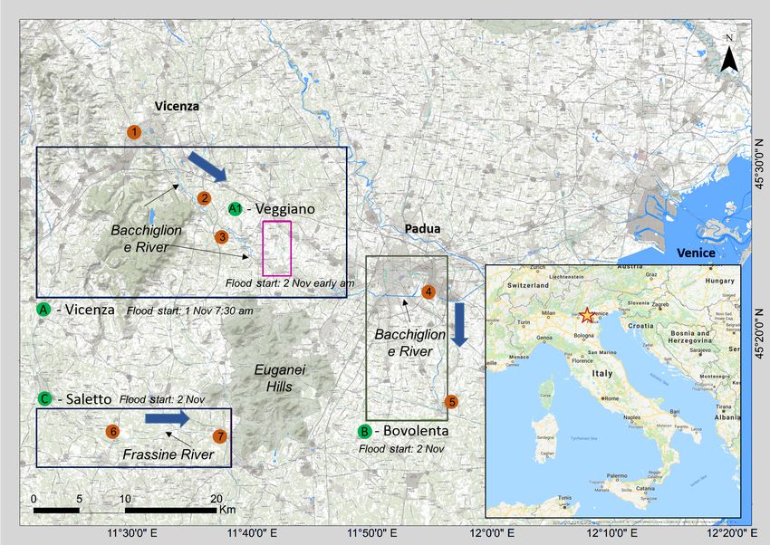
F. Cian et al.: Flood depth estimation by means of high-resolution SAR images and lidar data                                               3067

Figure 2. (a) Example of a detected flood polygon (light blue transparency) and relative flood boundary (red line). The dashed light blue line
indicates the actual flood boundary, not correctly detected by the SAR-based flood map due to presence of vegetation obscuring the flood
(cases indicated by the letter A) or due to radar shadow (cases indicated by the letter B). In the errors indicated by A, the elevation values
detected are lower than the actual ones. Vice versa, in the errors indicated by B, the elevation values detected are higher than the actual ones.
(b) Plot depicting the distribution function of the elevation along the boundary (red line). Areas indicated with A and B represent the values
associated with the errors as explained above. The two threshold values (at the fifth and the 95th percentiles) are used to exclude outliers.

elevation of the entire water surface contained in the poly-               distribution since an underestimation is more likely due to
gon itself; nevertheless, this is not happening due to different           the abovementioned sources of error.
error sources.                                                                Therefore, if we want to reliably estimate the correct wa-
   Figure 2a shows an example of a detected flooded polygon                ter elevation for each flooded polygon, we need to identify
(light blue transparency). Based on our theoretical assump-                and exclude outliers associated with omission errors (e.g.,
tions, this water surface should have a constant elevation. In             flood covered by vegetation) to commission errors (e.g.,
practice, this may not happen due to some sources of error                 radar shadow included in the flood map) or misalignments
(Fig. 2a). Specifically, the detected flood boundary (red line)            between SAR and DEM data.
may not correspond to the real boundary of the flood (dashed                  First, elevation values are extracted from the available
light blue line) due to (A) vegetation obscuring flooded areas             input DEM in correspondence with the boundary of each
leading to omission errors and (B) the nature of SAR images                flooded polygon individually. Then, the corresponding per-
(speckle, radar shadow, layover; Franceschetti and Lunari,                 centiles are computed (i.e., where a percentile denotes the
2018) that can lead to false alarms or omission errors. Un-                value below which a given percentage of observations falls in
certainties in the SAR-based flood map, errors in the DEM,                 the investigated group of observations) and values below the
and misalignment between the SAR data and the DEM can                      fifth and above the 95th percentiles are removed since, from
lead to further uncertainty in the detection of elevation values           extensive experimental analysis, this generally proved rather
along the boundary lines, resulting in outlier values under- or            effective for removing under- and overestimation errors. The
overestimating the real water elevation value. The plot re-                number of elevation points extracted depends on the length
ported in Fig. 2b shows the distribution (percentiles) of the              of the boundary of the flooded polygons and the horizontal
DEM elevation values along the boundary lines. The above-                  resolution of the DEM. Using a high-resolution DEM (e.g.,
mentioned errors (over- or/and underestimation) can be asso-               1 m horizontal resolution) may result in thousands of points
ciated with the values contained in areas A and B. It is more              for boundaries several kilometers in length.
likely to find outliers on the lower end of the elevation value               Next, given our hypothesis of a flat water surface, we have
                                                                           to check if the elevation value distribution is stable. Know-

www.nat-hazards-earth-syst-sci.net/18/3063/2018/                                   Nat. Hazards Earth Syst. Sci., 18, 3063–3084, 2018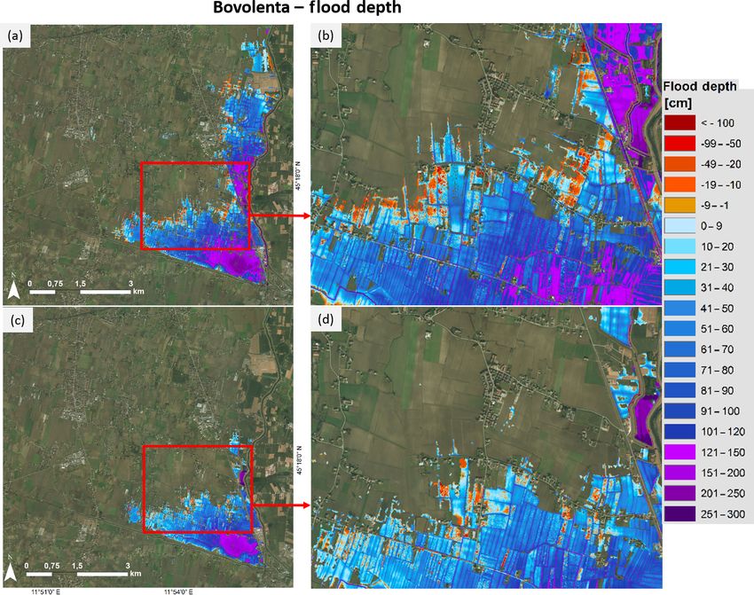
3068                        F. Cian et al.: Flood depth estimation by means of high-resolution SAR images and lidar data

ing that locally we can find a non-stable distribution (due to           n = 95
the abovementioned sources of error), starting from n = 95               for i = 0 to (n − 5) do
we iteratively compute, with step 1, the difference between                 if [Pn−i − P(n−5)−i ] ≤ 10 cm then
the DEM value corresponding to the nth and the (n − 5)th                        Water Surface Elevation = [Pn−i + P(n−5)−i ]/2
percentile. If the difference is greater than 10 cm, then the               else
process continues; otherwise we stop and compute the water                      i = i +1
elevation as the mean value between the extremes of the five-               end if
percentile interval analyzed at the last iteration. The idea is             if (n − 5 − i) = 50 then
                                                                                warning
to identify a plateau in the distribution that can represent the
                                                                            end if
correct water elevation.                                                 end for
   We start looking for the correct elevation from the high end
of the distribution for two reasons: (i) statistically there are         with P indicating the percentile and n the upper percentile
fewer outliers on this side of the distribution and (ii) because         threshold.
it is the highest correct value of water elevation that deter-
mines the overall water elevation for the considered flooded
polygon. The 95th percentile represents a good starting point,     can be unprecise. However, if this is not yet detected by the
able in most cases to exclude all the outliers present in one      threshold check, it can be easily detectable by analyzing at
single polygon.                                                    the resulting flood depth values. If inside a given polygon
   A step of five percentiles was found to be an optimal indi-     several negative values are obtained, this indicates an under-
cator of stability compared to the comparison of consecutive       estimation of the water elevation. Instead, if a given pixel is
percentiles. This adaptive threshold takes care of the different   associated with a flood depth much higher than its neighbors,
conditions of each single polygon and allows an increase in        then the water level may have been overestimated. There-
the precision of the method. As expected, the statistical dis-     fore, we select the polygons showing unexpected behaviors
tribution of elevation values is not identical for each bound-     and we compare them with a DEM-fill approach. The DEM
ary line. Therefore, a fixed threshold would have led to and       is filled up to the estimated water surface elevation. If the
increased uncertainty in the final water surface elevation es-     resulting polygon extent does not match with the observed
timation, especially in those cases in which flood polygons        flooded polygon, we manually look for the elevation value
have a non-regular geometry, which can overlap a complex           that best approximated the flood extent and set it as the water
topography or can encompass vegetation, roads, and built-up        elevation. Then we again compute the flood depth and reiter-
areas.                                                             ate the steps until we have a satisfying result.
   A threshold check is set on the 50th percentile, allowing
us to spot possible wrong estimations. In fact, an elevation
of the water surface below the 50th percentile indicates an        3     Data used and case study
exceptional behavior of the analyzed boundary line, which
would need dedicated investigation.                                3.1    Veneto flood 2010
   The water surface elevation estimation step is carried out
using a Python™ script including the ArcPy library. In this        Heavy rain concurrent with other adverse effects from 31 Oc-
script, we provide as inputs the flood map (shapefile for-         tober to 2 November 2010, in the Veneto region, northeast-
mat) and the DEM (raster format). The DEM is clipped us-           ern Italy, led to the flooding of 140 km2 of land with major
ing the boundary line of a flood polygon by means of the           damage to properties and infrastructures. The event was orig-
ArcPy function ExtractByMask. Then, the elevation values           inated by an Atlantic perturbation, which caused intense pre-
of this newly created raster are analyzed and their distribu-      cipitation over the whole area, with extremes in the pre-Alps
tion (percentiles) is computed. The procedure is repeated for      and piedmont areas. Local rainfall accumulation exceeded
each flooded polygon in the flood map, and the distribution        500 mm and the average widely surpassed 300 mm, leading
values of each polygon are added in the attribute table of the     to a serious hydraulic stress, especially in the area of Vicenza
shapefile. Finally, the algorithm selecting the optimal water      and the south of Padua. Sirocco wind, persistent on the sea
elevation value is summarized by the following:                    and inland, slowed the discharge of rivers into the sea. Early
                                                                   snow melt due to the warm temperature also added water to
2.3    Flood depth estimation                                      the rainfall.
                                                                      The first levee rupture in the study region occurred south
Finally, depth is determined for each flooded pixel as the dif-    of Vicenza in the afternoon of 1 November. Afterwards, the
ference between its DEM value and the water elevation esti-        flood propagated southeast to Veggiano, where the embank-
mated for the corresponding flooded polygon.                       ments of the Bacchiglione River were broken in the night
   In a few cases, in which the polygon geometry or the to-        between 1 and 2 November. During 2 November the Bac-
pography is non-regular, the estimation of the water level         chiglione banks also broke in the areas of Bovolenta, while

Nat. Hazards Earth Syst. Sci., 18, 3063–3084, 2018                           www.nat-hazards-earth-syst-sci.net/18/3063/2018/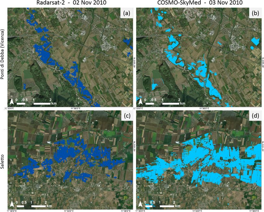
F. Cian et al.: Flood depth estimation by means of high-resolution SAR images and lidar data                                 3069

Table 1. List of COSMO-SkyMed SAR data (Stripmap 3 m) used             – the lidar digital terrain model (DTM) from the Venice
for deriving flood maps of the event.                                    Water Authority at 2 m resolution produced in 2004,
                                                                         which was employed for the Vicenza area of interest;
         Date                 Status      Acquisition
                                          time (UTC)                   – the lidar DTM from the Italian Ministry of the Environ-
                                                                         ment at 1m resolution produced in 2012, which has been
         31 October 2008      Reference         17:35
                                                                         used for the areas of Bovolenta and Saletto;
         28 April 2010        Reference         17:30
         29 August 2010       Reference         05:01                  – the 5 m resolution DTM available from the Veneto re-
         1 November 2010      Flood             05:01                    gion geodatabase, which was used for the whole area of
         3 November 2010      Flood             17:22
                                                                         interest for the cross comparison with the hydrodynamic
         4 November 2010      Flood             18:10
                                                                         model.
         6 November 2010      Flood             17:28
         7 November2010       Flood             05:13
                                                                     To validate the results, in absence of proper ground truth,
                                                                   we made use of different datasets that allowed us a qualitative
                                                                   assessment of our maps.
the area of Saletto started to be flooded due to the rupture of
the Frassine River banks in the same day (see Fig. 3). Based           – A simulation of the event by means of a hydrody-
on the analysis of SAR imagery (Cian et al., 2018), in the               namic model, in which flood extent was estimated for 3
area of Vicenza and Veggiano, the peak of the flood event                and 4 November using the 2DEF finite-element model
was estimated between 2 November (northwest of frame A                   (Viero et al., 2014) and flood depth was obtained as de-
in Fig. 3) and 3 November (placeholder “A1” in Fig. 3). In-              scribed by Viero et al. (2013). The simulation was com-
stead, in the Bovolenta area (frame B in Fig. 3) the flood               puted in order to correspond to the exact moment of the
extent peak was reached on 4 November, with a consequent                 SAR acquisition and it was performed using the DTM
decrease in water levels in the following days. The area of              of the Veneto region at 5 m resolution.
Saletto reached a maximum flood extent on 3 November.                  – A set of aerial photographs acquired on 1 Novem-
   Figure 4 shows the measurements of hydrometers along                  ber taken by the Fire Department of Vicenza covering
the Bacchiglione River (hydrometers 1 to 5) and along the                mainly the Vicenza area of interest was used.
Frassine River (hydrometers 6 and 7) (ARPAV, 2010). We
can notice how the flood wave moved from Vicenza (hy-                  – A set of in situ photographs taken from the Civil Pro-
drometer 1) to Bovolenta (hydrometer 5), in accordance with              tection Department on 1 and 2 November covering the
the analysis of SAR data, which estimated the maximum ex-                area of Saletto was used.
tent after the highest measurement of the hydrometers. Con-
                                                                       – A set of in situ photographs taken by the authors in 2017
cerning the Frassine River (hydrometers 6 and 7), we observe
                                                                         was used.
a similar behavior.
   Overall 262 municipalities were affected, leading to
roughly half a billion euros in damage, three fatalities, 3500     4     Results
displaced people, and more the 500 thousand people affected.
The flood also triggered hundreds of landslides in the moun-       4.1    Elevation value distribution
tainous surroundings, which led to more than 500 warnings
of instability phenomena received by the province soil pro-        As discussed above, the proposed methodology is based
tection division (Floris et al., 2012; Scorzini, 2017). This pa-   on the statistical analysis of the elevation values along the
per analyses three main areas as shown in Fig. 3: Vicenza          boundary lines of the estimated flooded polygons. Figure 5
and its surroundings (A), the Bovolenta area at the south of       shows the distribution (percentiles) of elevation values for 18
Padua (B), and the Saletto area at the south of Euganei Hills      randomly selected polygons in the Vicenza area of interest on
(a group of hills of volcanic origin that rise to heights of 300   3 November. As discussed in Sect. 2, on the tails of the dis-
to 600 m a few kilometers south of Padua) (C).                     tribution (below the fifth percentile and above the 95th per-
                                                                   centile) we can notice some irregularities, i.e., non-flat pro-
3.2   Data used                                                    files, in contrast to more stable behaviors in most of the cases
                                                                   in the central part of the profiles. The thresholds on the fifth
Flood maps were derived using CSK data, provided by the            and 95th percentiles cut out most of the outliers. By means of
Italian Space Agency, following the methodology proposed           the adaptive threshold starting from the 95th percentile, the
by Cian et al. (2018). Table 1 reports the complete list of        method is able to estimate the elevation of the water surface
scenes used.                                                       looking for a plateau on the distribution. It prevents the over-
   Additionally, different DEMs were used for estimating the       estimation of water elevation since it removes upper outliers,
flood depth:                                                       it prevents to underestimation by posing a limit on the lower

www.nat-hazards-earth-syst-sci.net/18/3063/2018/                           Nat. Hazards Earth Syst. Sci., 18, 3063–3084, 2018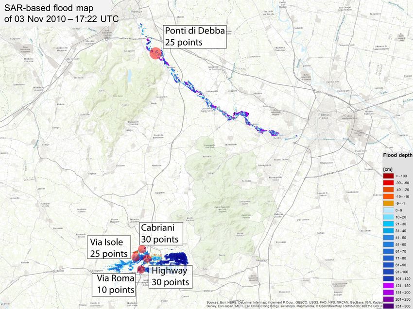
3070                          F. Cian et al.: Flood depth estimation by means of high-resolution SAR images and lidar data

Figure 3. Overview of the area affected by the 2010 flood event that occurred in the Veneto region (Italy). The three main areas of interest
are highlighted by the three frames: (A) Vicenza, (B) Bovolenta, and (C) Saletto. Placeholder A1 refers to the Veggiano area covered by
the hydrodynamic modeling used for comparison purposes. The numbers in orange circles indicate the location of the hydrometers, whose
measurements are reported in Fig. 4. For each frame the flood start date is reported along with the direction of the flood wave (blue arrows).

percentile and setting a condition on the slope of the profile           between the flood maps and the DEM). The threshold check
(elevation difference equal to or lower than 10 cm in a step             set at the 50th percentile detects the first problem, while the
of five percentiles). Less regular profiles can be seen in the           second is detected by looking at high value of flood depth
plot, like the one indicated by arrows A and B in Fig. 5. The            (>2 m) or by finding discontinuities between neighboring
irregularity is due to errors in the flood map, such as when             polygons in the estimated surface water elevation. For those
vegetation obscures part of the flooded area, when there is              few cases, it is necessary to intervene manually as it is not
a misalignment between the flood map and the DEM, when                   possible to estimate the right elevation simply looking at this
flooded polygons exhibit a non-regular geometry, or when                 statistic, as described at the end of Sect. 2.
the DEM along the flood boundaries has a complex topogra-
phy. In these cases (less than 3 %), the proposed methodol-              4.2    Flood depth estimation
ogy might not result in reliable estimations. In fact, the ele-
vation can exhibit two problems: (i) it never shows a stable             Flood depth was computed for the three areas of interest in-
value along the distribution (no plateau is found) and the wa-           dicated in Fig. 3. Flood depth was estimated for the whole
ter elevation is associated with the 50th percentile, and (ii) it        flooded area except for a small portion of Veggiano area (a
presents a plateau at a higher elevation with respect to the             portion of the A.1 area indicated in Fig. 3), where lidar data
real water surface elevation, resulting in an overestimation of          were not available. Figure 6 shows the results for the Vi-
the flood depth (this may rarely happen for example when                 cenza area of interest. Specifically, Fig. 6a shows the flood
the flood map crosses over roads or river banks at higher ele-           maps for 3 November and Fig. 6b the lidar extent, which cov-
vation due to inaccuracies of the flood map or misalignment              ers the entire flood with the exception of the central part of
                                                                         the map (the portion of the Veggiano area mentioned above).

Nat. Hazards Earth Syst. Sci., 18, 3063–3084, 2018                                www.nat-hazards-earth-syst-sci.net/18/3063/2018/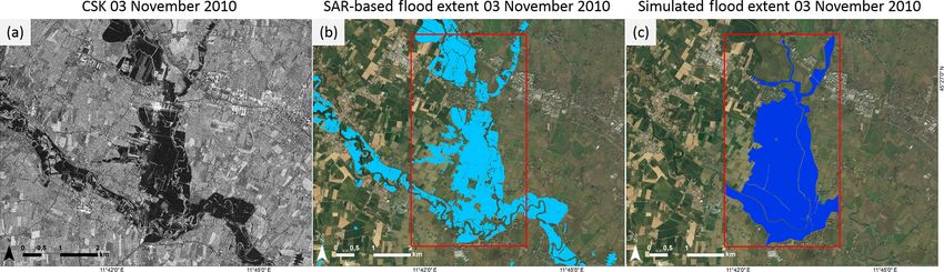
F. Cian et al.: Flood depth estimation by means of high-resolution SAR images and lidar data 3071
Figure 4. Measurements of hydrometers during the period of the investigated flood event. The flow of the Bacchiglione River (hydrometers
1 to 5) goes towards the southeast, i.e., from hydrometers 1 to 5. The flow of the Frassine River (hydrometers 6 and 7) goes towards the east,
i.e., from hydrometers 6 to 7. In both cases, the measurements show the dynamic of the flood, which followed the stream of the river.
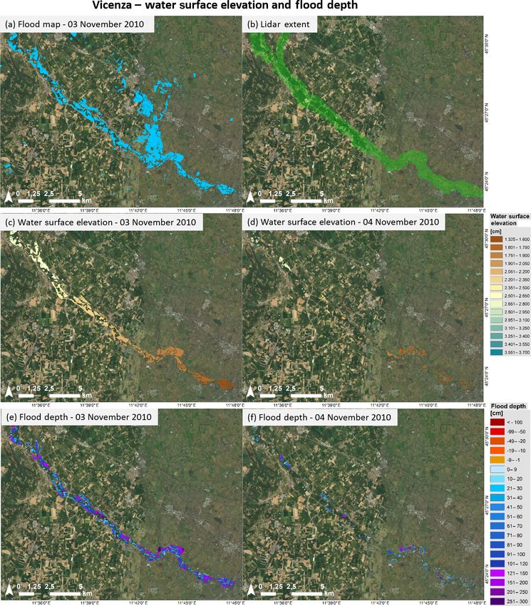
Figure 6c and e show, respectively, water surface elevation Figure 7 shows the flood depth for the Bovolenta area of
and flood depth for 3 November. Figure 6d and f show wa- interest on (a) 4 and (c) 6 November. Also in this case, we
ter surface elevation and flood depth for 4 November. The can notice the receding of flood extent between the two dates.
dynamics of the event, i.e., the receding of water from 3 to Figure 7b and d show a zoom of the results, in which the high
4 November, can be noticed where extent and depth of the level of detail can be appreciated.
flood decrease. The flooded area extends for several kilome- Figure 8 shows the results for the Saletto area of interest
ters along the Bacchiglione River where the terrain eleva- on (a) 3, (b) 4, (c) 6, and (d) 7 November. In this case, the
tion decreases gradually from the northwest to the southeast. evolution of the event, in particular the decrease in flood ex-
Since we estimate water elevation for each single polygon, tent and depth is even clearer given the higher number of
we are able to also take into consideration the slope of the observations available.
river. This can be noted in the overall decrease in water sur- As is evident from the depth maps and the relative scales,
face elevation values in Fig. 6c and d. there can be negative values of flood depth, which in most of
For types of floods similar to this, the hypothesis of a flat the cases occur at the proximity of the boundaries of flooded
water surface inside a single polygon is a good approxima- polygons. These most likely indicate an underestimation of
tion since the flood evolution is slow and therefore water sur- the water surface elevation, even if false alarms in the flood
face can be considered flat. This is especially true in the case map can also induce the same problem. However, the neg-
of the Bovolenta and Saletto areas of interest where the flood ative values are in most of the cases of the order of a few
extent was limited and the topography relatively simple. centimeters (less than 10 cm) and these pixels can be consid-
ered very shallow water.
www.nat-hazards-earth-syst-sci.net/18/3063/2018/ Nat. Hazards Earth Syst. Sci., 18, 3063–3084, 2018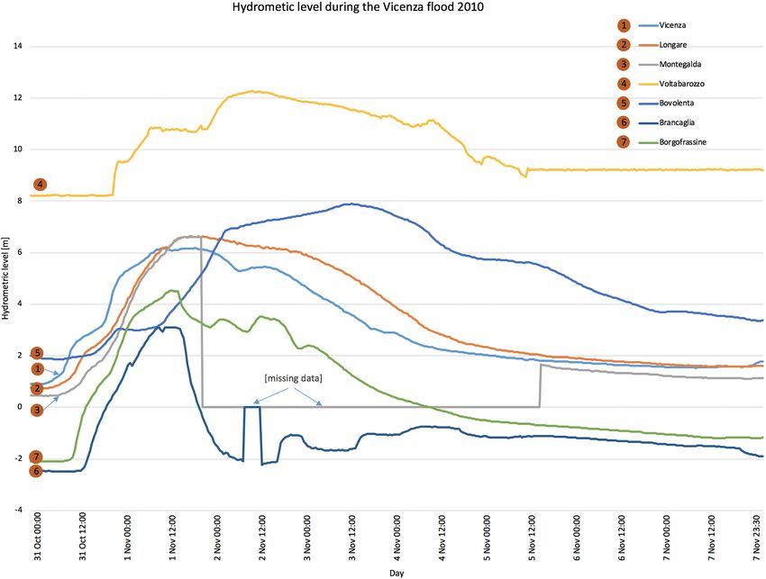
3072                          F. Cian et al.: Flood depth estimation by means of high-resolution SAR images and lidar data

Figure 5. Elevation value distribution (percentiles) for a random selection of the flood polygon’s boundaries in the Vicenza area on 3 Novem-
ber. The 95th and fifth percentile thresholds are highlighted. Arrows “A” and “B” indicate less regular profiles, for which the proposed
methodology is less effective. In these cases (less than 3 % of the total) a manual intervention is necessary.

5     Assessment and discussions                                         of the aerial photos acquisition, (2) analysis of water ele-
                                                                         vation obtained using the proposed SAR-based method, and
5.1    Assessment with aerial photos                                     (3) cross comparison of the two values.
                                                                            Concerning step 1, we made use of (i) a DEM-fill tech-
                                                                         nique and (ii) data acquired during fieldwork in late 2017.
Ground truth data consist of aerial photographs taken on                 DEM-fill consists of filling the DEM up to the elevation that
1 November right after the beginning of the event and of field           gives a flood extent similar to the one displayed by the pho-
pictures taken on 1 and 2 November by civil protection. Un-              tos, which will be the estimated water elevation. In the field-
fortunately, they do not match the dates and time of satel-              work, we measured the height of the water plane on features
lite acquisitions; therefore they cannot be used as a proper             recognizable in the aerial photos. These measurements added
validation dataset. However, given the slow dynamic of the               to the DEM value in the same location, allowing the estima-
flood, they can provide very useful information about the wa-            tion of water elevation. Averaging these two values allows
ter level, which can be estimated and compared with the re-              the estimation of the water elevation at the moment of acqui-
sults of our method and therefore provide an assessment of               sition of the aerial photos, which can be compared with the
the results. To prove this, in Fig. 9 we show a comparison of            results given by the proposed SAR-based method.
flood extents derived for 2 November from 25 m resolution                   Concerning step 2, SAR-based results are analyzed in
RADARSAT-2 data and for 3 November from 5 m resolution                   comparison with a DEM-fill method to understand the con-
CSK imagery. The lower resolution of RADARSAT-2 does                     sistence of flood depth values in relation to the extent of
not allow extraction of the same level of detail of the map              DEM-based simulated flood.
based on CSK data, but it is enough to show that the sta-                   Concerning step 3, the cross comparison is performed by
tus of the flooded areas on the two consecutive days is very             comparing water elevation obtained in steps 1 and 2.
similar. Therefore, it makes sense to use the available aerial              The assessment was performed for the flood depth maps of
photographs for assessing the results, keeping in mind a pos-            3 November, the date of the first high-resolution SAR image
sible change in the flood status between the two situations. In          available after the acquisition of the aerial photos.
particular, from the image we can notice that for the Vicenza               Panel I of Fig. 10 shows flood extent and depth (Fig. 10a)
area (Fig. 9a and b) the flood receded from 2 to 3 November,             on 3 November at 17:22 UTC in the area of Ponti di Debba,
while for the Saletto area (Fig. 9c and d) it expanded.                  south of the city of Vicenza, derived from the CSK SAR im-
   The assessment is carried out in three different steps:               age shown in Fig. 10b. Panel II of Fig. 10 shows an aerial
(1) estimation of water elevation corresponding to the dates

Nat. Hazards Earth Syst. Sci., 18, 3063–3084, 2018                               www.nat-hazards-earth-syst-sci.net/18/3063/2018/
F. Cian et al.: Flood depth estimation by means of high-resolution SAR images and lidar data 3073 Figure 6. Water surface elevation and flood depth estimation for the Vicenza area of interest on 3 and 4 November. Panel (a) shows the flood map for 3 November and (b) the extent of the lidar data, which do not completely cover the flooded areas. Panels (c) and (d) show water surface elevation, and panels (e) and (f) show flood depth, respectively, for 3 and 4 November. Reddish values in (e) and (f) indicate negative flood depth and therefore an error in the estimation of the water surface elevation (underestimation). www.nat-hazards-earth-syst-sci.net/18/3063/2018/ Nat. Hazards Earth Syst. Sci., 18, 3063–3084, 2018
3074                         F. Cian et al.: Flood depth estimation by means of high-resolution SAR images and lidar data

Figure 7. Flood depth for the Bovolenta area of study on (a) 4 November and (c) 6 November. Panels (b) and (d) show a zoom of the results,
highlighting the high level of detail achievable. Reddish pixels represent the error in the water level estimation.

photo and fieldwork of the same area. Figure 10c shows the                Figure 10f shows that with a water elevation of 28 m, based
aerial photo acquired on 1 November at 14:00 UTC, in which             on the DEM we obtain a very similar water extent of the one
three areas are highlighted: area 1 (zoom in 1.A) for which            observed in the aerial photo. If we set a water level of 27.45 m
the proposed method detects no flood on 3 November and                 (Fig. 10e), the value estimated from fieldwork, we would ob-
the DEM-fill method estimate of a water elevation of 28 m;             tain a slightly underestimated flood extent compared to the
area 2 (zoom in 2.A) for which our method estimates a water            one observed in the aerial photo. From this analysis, we can
level of 26.98 m and the fieldwork data 27.46 m (27.06 m ele-          estimate a water level on 1 November of 27.72 m (average
vation given by the DEM plus 0.4 m of flood depth estimated            between 27.45 and 28 m).
from fieldwork); area 3 (zoom in 3.A) for which our method                Looking at Fig. 10d, we can observe that the flood extent
detects no flood and the fieldwork data 27.45 m (27 m eleva-           resulting with a water level of 26.98 m, the same estimated
tion given by the DEM plus 0.45 m of flood depth estimated             with our method, is very similar to the extent extracted from
from fieldwork). Panel III of Fig. 10 shows the flood extent           the SAR image. A similar extent confirms the goodness of
derived with the DEM-fill method for different water levels:           the SAR-based flood map, while the estimation of the wa-
Fig. 10d with a water level equal 26.98 m corresponding to             ter level, 26.98 m, is comparable to the value estimated from
the level estimated by our method; Fig. 10e with a water level         the aerial photo and relative to 2 days before the SAR ac-
equal to 27.45 m, corresponding to the water level estimated           quisition. This would mean a decrease in the water level of
by fieldwork data; and Fig. 10f with a water level equal to            0.74 m in 2 days. The reduction of flood extent in this area
28 m, corresponding to the level estimated by the DEM-fill             from 2 to 3 November is also confirmed by RADARSAT-2
method in order to obtain the same flood extent of the aerial          acquisition as we can see in Fig. 9a and b.
photo.                                                                    Panel I of Fig. 11 shows flood extent and depth (Fig. 11a)
                                                                       on 3 November at 17:22 UTC in the area of Via Isole, in

Nat. Hazards Earth Syst. Sci., 18, 3063–3084, 2018                              www.nat-hazards-earth-syst-sci.net/18/3063/2018/
F. Cian et al.: Flood depth estimation by means of high-resolution SAR images and lidar data 3075
Figure 8. Flood depth for the area of interest of Saletto on (a) 3, (b) 4, (c) 6, and (d) 7 November.
the Saletto area, derived from the CSK SAR image shown obtain the same flood extent compared to the one observed in
in Fig. 11b. Panel II of Fig. 11 shows an aerial photo and the aerial photo. From this analysis, we can estimate a water
fieldwork of the same area. Figure 11c shows the aerial photo level on 1 November of 11.38 m.
acquired on 1 November at about 14:50 UTC, in which two Looking at Fig. 11d, we can observe that the flood extent
areas are highlighted: area 1 (zoom in 1.A) for which the pro- resulting with a water level of 11.6 m, the same estimated
posed method detects a water elevation of 11.6 m, the DEM- with the proposed method, is very similar to the one observed
fill method estimates a water elevation of 11.4 m, and the in the SAR image.
fieldwork data estimates 11.38 m (10.7 m elevation given by Also in this case, an increase of 0.2 m from 2 to
the DEM plus 0.68 m of flood depth estimated from field- 3 November is consistent with the situation observed in SAR
work); area 2 (zoom in 2.A) for which the proposed method acquisitions as shown in Fig. 9c and d.
estimates a water elevation of 11.6 m and the fieldwork data Buildings in the central north side of the image are cate-
11.33 m (10.93 m elevation given by the DEM plus 0.4 m of gorized as flooded by the DEM-fill method in contrast to the
flood depth estimated from fieldwork). Panel III of Fig. 11 SAR-based maps. It is worth noticing that SAR data do not
shows the flood extent derived with the DEM-fill method for allow extraction of flooded areas between buildings, where
different water levels: Fig. 11d with a water level equal to a mechanism of double bounce occurs, making the radar
11.6 m corresponding to the elevation estimated by the pro- backscatter increase rather than decrease. However, we have
posed method; Fig. 11e with a water level equal to 11.38 m, no evidence that this specific area was actually flooded.
corresponding to the water elevation estimated by field work; The same approach was followed for a total of 120 points
Fig. 11f with water level equal to 11.4 m, corresponding to distributed in the Vicenza (25 points) and Saletto areas of
the level estimated by the DEM-fill method in order to ob- study (95 points) as shown in Fig. 12. These points were se-
tain the same flood extent of the aerial photo. lected based on recognizable features in the aerial or field-
Figure 11f shows that with a water elevation of 11.4 m, work photos of 1 and 2 November. These points belonged
based on the DEM we obtain a water extent very similar to to different flood polygons in the SAR-based flood map. For
the one observed in the aerial photo. If we set a water level each point, we computed the difference between the water
of 11.38 m (Fig. 11e), the value estimated from fieldwork, we elevation estimated for 1 or 2 November based on aerial or
www.nat-hazards-earth-syst-sci.net/18/3063/2018/ Nat. Hazards Earth Syst. Sci., 18, 3063–3084, 20183076 F. Cian et al.: Flood depth estimation by means of high-resolution SAR images and lidar data
Figure 9. Comparison between RADARSAT-2 (2 November 2010) and COSMO-SkyMed flood maps (3 November 2010). RADARSAT-2
has a lower resolution (25 m) compared to COSMO-SkyMed (5 m), which provides a coarser flood map. We can see by the comparison of
the two maps that the flood has a comparable extent on the two days. In particular, from the image we can notice that for the Vicenza area
(Fig. 9a and b) the flood has receded from 2 to 3 November, while for the Saletto area (Fig. 9c and d) it has expanded.
fieldwork photos (step 1 of the assessment process) and the 5.2 Cross comparison: hydrodynamic modeling
water elevation estimated from the SAR image for 3 Novem-
ber. For the area of Vicenza we obtained an average differ-
ence of +53 cm. This difference is consistent with the ob- Flood depth obtained with the presented methodology was
served change of flood depth (decrease) from 1 and 3 Novem- compared with the one derived using the hydrodynamic
ber. For the area of Saletto we obtained an average differ- model presented in Viero et al. (2013). The simulation was
ence of −47 cm, a value that is consistent with the increase available for the area of Veggiano (area A1 in Fig. 3) and Bo-
in flood depth observed from 1 and November 3. volenta (area B in Fig. 3) on 3 and 4 November at the same
The differences are mainly due to the different timing of time of the SAR acquisitions over the same areas. It made
observation between the SAR image and the aerial and field- use of the DTM at 5 m resolution of the Veneto region geo-
work photos. However, a source of errors is also intrinsic in database; therefore the same DTM has been used with the
the SAR method. In fact, we can have false alarms or a false proposed methodology to derive meaningful results for com-
negative in the flood map (overestimation of flood extent due parison.
to radar shadow, or flood underestimation due to vegetation The first row of panels in Fig. 13 shows the simulated
on top of flood areas) or misalignment between the DEM and flood depth (a), the SAR-based estimated flood depth (b), and
the SAR data, which could be a geolocation error or an effect the difference between the two (c) for the Veggiano area on
of different resolutions between the two datasets. 3 November 2010. The second row, Fig. 13d–f, shows the
same series of results for the same area on 4 November. The
third row, Fig. 13g–i, shows the same series of results for the
Bovolenta area on 4 November.
Nat. Hazards Earth Syst. Sci., 18, 3063–3084, 2018 www.nat-hazards-earth-syst-sci.net/18/3063/2018/F. Cian et al.: Flood depth estimation by means of high-resolution SAR images and lidar data 3077 Figure 10. Flood depth on 3 November over Ponti di Debba in the Vicenza area of interest; panel I shows (a) flood depth in the area analyzed; (b) CSK image acquired on 3 November at 17:22 UTC from where the flood map has been derived; panel II shows (c) an aerial view of the event acquired on 1 November at about 14:00 UTC with zooms on three areas (1.A, 2.A, 3.A) with relative fieldwork images (2.B and 3.B); panel III shows the flood extent derived with the DEM-fill method for different water levels: (d) with a water level equal to 26.98 m corresponding to the level estimated by the proposed method; (e) with a water level equal to 27.45 m corresponding to the water level estimated by fieldwork data; (f) with a water level equal to 28 m corresponding to the level estimated by the DEM-fill method in order to obtain the same flood extent of the aerial photo. www.nat-hazards-earth-syst-sci.net/18/3063/2018/ Nat. Hazards Earth Syst. Sci., 18, 3063–3084, 2018
3078                          F. Cian et al.: Flood depth estimation by means of high-resolution SAR images and lidar data

Figure 11. Flood depth on 3 November over Via Isole in the Saletto area of interest; panel I shows (a) flood depth in the area analyzed;
(b) CSK image acquired on 3 November at 17:22 UTC from where the flood map has been derived; panel II shows (c) an aerial view of
the event acquired on 1 November at about 14:50 UTC with zooms on two areas (1.A, 2.A) with relative fieldwork images (2.B and 3.B);
panel III shows the flood extent derived with the DEM-fill method for different water levels: Fig. 11d with a water level equal to 11.6 m
corresponding to the elevation estimated by the proposed method; Fig. 11e with a water level equal to 11.38 m corresponding to the water
elevation estimated by fieldwork for area 1; Fig. 11f with a water level equal to 11.4 m corresponding to the level estimated by the DEM-fill
method in order to obtain the same flood extent of the aerial photo.

Nat. Hazards Earth Syst. Sci., 18, 3063–3084, 2018                               www.nat-hazards-earth-syst-sci.net/18/3063/2018/
F. Cian et al.: Flood depth estimation by means of high-resolution SAR images and lidar data                                              3079

Figure 12. Distribution of the validation points selected for flood depth assessment: a total of 120 validation points collected in the Vicenza
and Saletto areas (i.e., 25 and 95, respectively) have been selected based on recognizable features in the aerial and fieldwork photos available
for 1 and 2 November. The reported SAR-based flood depth map used for the assessment refers to 3 November 2010.

   Differences of two types can be seen between the two ap-               ally we can observe an overestimation of flood depth by the
proaches: (i) different flood extent and (ii) different flood             hydrodynamic model, which overestimates the flood extent.
depth values between the model-based result and the SAR-                  In the case of Veggiano on both dates (Fig. 13c and f), the
based one. Concerning the first type of difference, Fig. 14               difference is greater than 1 m only in a small portion of the
shows the SAR image (a) from which the SAR-based flood                    image (
3080                       F. Cian et al.: Flood depth estimation by means of high-resolution SAR images and lidar data

Table 2. Flood extent cross comparison between SAR-based extent and hydrodynamic model-based extent.

                     Date – area                Only hydrodynamic      Only SAR-based        Agreement between
                                                model extent (km2 )       extent (km2 )    the two extents (km2 )
                     3 November – Veggiano                    6.81                 5.86                     4.33
                     4 November – Veggiano                    4.87                 3.82                     2.77
                     4 November – Bovolenta                  15.63                 8.48                     7.98

Table 3. Comparison between flood depth obtained with the hydrodynamic model and the proposed methodology.

                              Date – area                Mean difference      Mean absolute    RMSD
                                                                    (cm)     difference (cm)    (cm)
                              3 November – Veggiano                   −27                 42        55
                              4 November – Veggiano                   −63                 68        73
                              4 November – Bovolenta                  −37                 62        79

consistent, about 7 km2 ; i.e., the model reports about 2 times       the area of Vicenza, due mainly to the decrease in water
the extent of the SAR observation. These numbers confirm              level from 1 November (date of aerial images) to 3 Novem-
the overestimation of the hydrodynamic model. The reasons             ber (date of SAR acquisition), and (ii) an average overesti-
for this difference can vary. On the one hand, areas reported         mation of 47 cm for the area of Saletto, due mainly to the
as flooded in the simulation could have been in truth pro-            increase in water level from 1 November (date of aerial im-
tected by barriers not taken into consideration by the model,         ages) to 3 November (date of SAR acquisition) in this part of
hence leading to an overestimation of the simulated flood ex-         the flood.
tent. On the other hand, the SAR-based maps might experi-                In comparison with hydrodynamic models, this method-
ence some underestimation in the presence of urban or veg-            ology is more easily implemented since less information is
etated flooded areas (where the radar backscattering might            needed: a stack of SAR images (before and after the event)
increases due to specific multiple bouncing).                         and a DEM. Hydrodynamic models need additional informa-
   Table 3 instead numerically compares the flood depth ob-           tion, such as inflow discharges and values for roughness pa-
tained with the two methods. The root-mean-square differ-             rameters, in order to derive depth and in case of a desired
ence (RMSD) shows a value of 55 cm in the area of Veg-                higher precision also precipitation data, information about
giano on 3 November, 73 cm on 4 November, and 79 cm in                the soil, number and location of water pumps, etc.
the area of Bovolenta on 4 November. Once again, the num-                The comparison with results obtained with a hydrody-
bers confirm the qualitative analysis and were expected given         namic model gives relatively good correspondence, the main
the overestimation of the flood extent by the model.                  difference being the different flood extent estimated by the
                                                                      model, which leads to a generally higher depth estimation.
                                                                      The model shows less accuracy together with a more com-
6   Conclusions                                                       plex utilization due to the additional data required to run it.
                                                                         However, it must be taken into consideration that satellite
In this paper, we showed a methodology for assessing flood            observations allow us to outline the flooded area and estimate
depth based on a statistical analysis of elevation data along         the water depth at the specific date and time of their acqui-
the boundary lines of flooded areas. Starting from flood ex-          sition, which do not necessarily correspond to the maximum
tent maps and using high-resolution DEM, water elevation              flood extent and water depth. If the images are acquired far
can be estimated and therefore flood depth computed. The              from the flood peak (either before or after), the estimated ex-
methodology may become suitable for operational mode. In              tent and depth will underestimate the worst situation that oc-
fact, it meets the ideal requirements as indicated by Brown et        curred during the event.
al. (2016): accurate, simple to use also for non-Geographical            In comparison to existing methodologies in the literature
Information System and remote sensing experts, easily appli-          based on SAR data, the method we present is simple since it
cable to different satellite data (SAR and optical), and quick        requires only the flood extent map and a DEM as inputs, it is
to apply.                                                             based on an algorithm that does not require strong capacity
   The results have been assessed through aerial and field-           in terms of computation and manual interaction, and it is able
work images acquired during the event. The assessment, car-           to handle the uncertainties of the SAR-based flood maps.
ried out on 120 pints distributed in the areas of Vicenza and
Saletto, shows (i) an average underestimation of 53 cm for

Nat. Hazards Earth Syst. Sci., 18, 3063–3084, 2018                           www.nat-hazards-earth-syst-sci.net/18/3063/2018/
You can also read