What's streamflow got to do with it? A probabilistic simulation of the competing oceanographic and fluvial processes driving extreme along-river ...
←
→
Page content transcription
If your browser does not render page correctly, please read the page content below
Nat. Hazards Earth Syst. Sci., 19, 1415–1431, 2019
https://doi.org/10.5194/nhess-19-1415-2019
© Author(s) 2019. This work is distributed under
the Creative Commons Attribution 4.0 License.

What’s streamflow got to do with it? A probabilistic
simulation of the competing oceanographic and fluvial
processes driving extreme along-river water levels
Katherine A. Serafin1,2 , Peter Ruggiero1 , Kai Parker3 , and David F. Hill3
1 College of Earth, Ocean, and Atmospheric Sciences, Oregon State University, Corvallis, OR, USA
2 Department  of Geophysics, Stanford University, Stanford, CA, USA
3 School of Civil and Construction Engineering, Oregon State University, Corvallis, OR, USA

Correspondence: Katherine A. Serafin (kserafin@stanford.edu)

Received: 14 November 2018 – Discussion started: 9 January 2019
Accepted: 24 May 2019 – Published: 16 July 2019

Abstract. Extreme water levels generating flooding in estu-      1   Introduction
arine and coastal environments are often driven by compound
events, where many individual processes such as waves,           Coincident or compound events are a combination of phys-
storm surge, streamflow, and tides coincide. Despite this, ex-   ical processes in which the individual variables may or may
treme water levels are typically modeled in isolated open-       not be extreme; however, the result is an extreme event with a
coast or estuarine environments, potentially mischaracteriz-     significant impact (Zscheischler et al., 2018; Bevacqua et al.,
ing the true risk of flooding facing coastal communities. This   2017; Wahl et al., 2015; Leonard et al., 2014). Flooding is
paper explores the variability of extreme water levels near      often caused by compound events, where multiple factors
the tribal community of La Push, within the Quileute In-         impact both open-coast and estuarine environments. Storm
dian Reservation on the Washington state coast, where a river    events, for example, often generate concurrently large waves,
signal is apparent in tide gauge measurements during high-       heavy precipitation driving increased streamflow, and high
discharge events. To estimate the influence of multiple forc-    storm surges, making the relative contribution of the actual
ings on high water levels a hybrid modeling framework is         drivers of extreme water levels difficult to interpret. Studies
developed, where probabilistic simulations of joint still wa-    at the global (e.g., Ward et al., 2018), national (e.g., Wahl
ter level and river discharge occurrences are merged with a      et al., 2015; Svensson and Jones, 2002; Zheng et al., 2013)
hydraulic model that simulates along-river water levels. This    and regional scale (e.g., Odigie and Warrick, 2017; Mof-
methodology produces along-river water levels from thou-         takhari et al., 2017) have evaluated the likelihood for vari-
sands of combinations of events not necessarily captured in      ables such as high river flow and precipitation to occur dur-
the observational records. We show that the 100-year still wa-   ing high coastal water levels, demonstrating that dependen-
ter level event and the 100-year discharge event do not always   cies often exist between these individual processes.
produce the 100-year along-river water level. Furthermore,          Around river mouths, the elevation of the water level mea-
along specific sections of river, both still water level and     sured by tide gauges, or the still water level (SWL), varies
discharge are necessary for producing the 100-year along-        depending on the mean sea level, tidal stage, and the non-
river water level. Understanding the relative forcing driving    tidal residual contributors which may include the follow-
extreme water levels along an ocean-to-river gradient will       ing forcings: storm surge, seasonally induced thermal ex-
help communities within inlets better understand their risk to   pansion (Tsimplis and Woodworth, 1994), the geostrophic
the compounding impacts of various environmental forcing,        effects of currents (Chelton and Enfield, 1986), wave setup
which is important for increasing their resilience to future     (Sweet et al., 2015; Vetter et al., 2010), and river discharge.
flooding events.                                                 Most commonly, estimates of nontidal residuals are deter-
                                                                 mined by subtracting predicted tides from the measured wa-

Published by Copernicus Publications on behalf of the European Geosciences Union.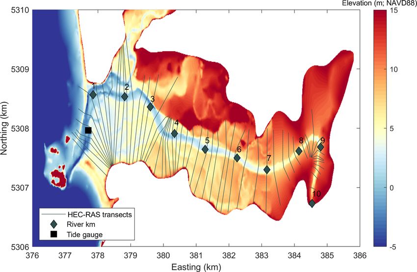
1416                                                                               K. A. Serafin et al.: Competing processes

ter levels. However, residuals computed in this way often         model, which allows for multiple synthetic representations
contain artifacts of the subtraction process from phase shifts    of joint ocean and riverine processes that may not have oc-
in the tidal signal and/or timing errors (Horsburgh and Wil-      curred in the relatively short observational records. Next, a
son, 2007). Another approach for extracting the nontidal          one-dimensional hydraulic model is used to simulate water
residual is through the skew surge, which is the absolute dif-    surface elevations along a 10 km stretch of river. Surrogate
ference between the maximum observed water level and the          models are generated from the hydraulic model simulations
predicted tidal high water (de Vries et al., 1995; Williams       and used to extract along-river water levels for each prob-
et al., 2016; Mawdsley and Haigh, 2016). While this method-       abilistic joint occurrence of SWL and river discharge in a
ology removes the influence of tide–surge interaction from        computationally efficient manner. Rather than determining
the nontidal residual magnitude, it does not differentiate be-    the along-river return level from an equivalent return level
tween the many factors contributing to the water level, an        forcing (e.g., the 100-year discharge event drives the 100-
important step for distinguishing when and why high water,        year water level), spatially varying along-river return levels
and thus flooding, is likely to occur.                            are extracted and matched to the driving boundary condi-
   Hydrodynamic and hydraulic models have recently been           tions. This technique allows for a spatially explicit analysis
used in attempts to quantify the relative importance of river-    of the ocean and river conditions generating extreme water
and ocean-forced water levels to flooding. The nonlinear cou-     levels.
pling of wind- and pressure-driven storm surge, tides, wave-         The following sections describe the study area, present the
driven setup, and riverine flows has been found to be a vi-       hybrid modeling framework linking oceanographic and river-
tal contributor to overall water level elevation (Bunya et al.,   ine systems, and evaluate the compounding drivers of along-
2010). Furthermore, river discharge is often found to inter-      river extreme water levels.
act nonlinearly with storm surge (Bilskie and Hagen, 2018),
exacerbating the impacts of coastal flooding (Olbert et al.,
2017), which suggests that the extent or magnitude of flood-      2   Study area
ing is often underpredicted when both river and oceanic pro-
cesses are not modeled (Bilskie and Hagen, 2018; Kumbier          The Quillayute River is located in Washington state along
et al., 2018; Chen and Liu, 2014). The computational demand       the US west coast and drains approximately 1630 km2 of
of two- and three-dimensional hydrodynamic models, how-           the northwestern Olympic Peninsula into the Pacific Ocean
ever, typically precludes a large amount of events to be ex-      (Czuba et al., 2010). The Quillayute River is approximately
amined. Therefore, while accurately modeling the physics of       10 km long; is formed by the confluence of the Bogachiel
the combined forcings, researchers taking this approach are       and Sol Duc rivers (Fig. 1); and enters the Pacific Ocean
often limited to modeling only a select number of boundary        at La Push, Washington, home to the Quileute Tribe. The
conditions. On the other hand, statistical models allow for       Quileute Indian Reservation is approximately 4 km2 and the
the investigation of compound water levels through the sim-       majority of community infrastructure sits at the river mouth,
ulation of combinations of dependent events which may not         bordering the river and open coast. The Quileute Harbor Ma-
have been physically realized in observational records (Be-       rina is also situated just inside the river mouth and is the
vacqua et al., 2017; van den Hurk et al., 2015). In addition,     only port between Neah Bay and Westport, Washington. Ri-
researchers have recently begun to generate hybrid models         alto Spit, which connects Rialto Beach to Little James Island,
that link statistical and physical modeling approaches for un-    contains a rocky revetment which protects the marina and the
derstanding compound flood events (Moftakhari et al., 2019;       community from ocean and storm wave impact.
Couasnon et al., 2018). Similar to the results solely from           The Quillayute River is a natural, unstabilized river that
hydrodynamic and hydraulic models, statistical and hybrid         is relatively straight at the confluence of the Bogachiel and
modeling strategies show that simplifications of the depen-       Sol Duc rivers and increases in sinuosity moving towards
dence between multiple forcings may lead to an underesti-         the river mouth. Channel-bed materials are coarse (gravel
mation of flood risk.                                             and cobble) in the free-flowing channels and dominated by
   This study explores the influence of oceanographic and         sand in the small estuary (Czuba et al., 2010). Upstream of
riverine processes on extreme water levels along a coastal        river kilometer 3 there are numerous point bars and bends in
river where there is a substantial river signal recorded in       the river. Between river kilometer 1.5 and 3, the Quillayute
the tide gauge. In order to better understand the river- and      River is braided with several side channels, usually contain-
ocean-forced water levels at this location, a hybrid methodol-    ing woody debris (Czuba et al., 2010). The channel is straight
ogy is developed for linking statistical simulations of ocean     near the river mouth and is confined by the Rialto Spit revet-
and river boundary conditions with a hydraulic model that         ment before draining into the Pacific Ocean.
simulates along-river water levels. First, river-influenced wa-      The oceanic climate of the coastal Pacific North-
ter levels are defined and removed from SWLs. Then, both          west (PNW) is cool and wet with a small range in temper-
river discharge and river-influenced water levels are incor-      ature variation and the majority of rainfall between October
porated into a nonstationary, probabilistic total water level     and May. Four river basins, the Sol Duc, Bogachiel, Calawah,

Nat. Hazards Earth Syst. Sci., 19, 1415–1431, 2019                       www.nat-hazards-earth-syst-sci.net/19/1415/2019/
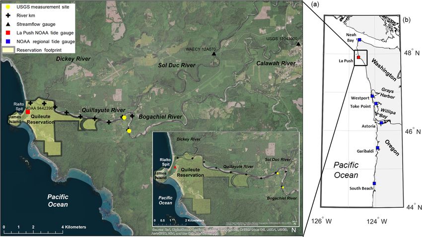
K. A. Serafin et al.: Competing processes                                                                                         1417

Figure 1. Map of study area (a), which is denoted on the regional map (b) in the black box. The La Push tide gauge is represented as
a red square while other regional tide gauges are represented as blue squares. The Calawah and Sol Duc River gauges are represented as
black triangles, and USGS measurement sites from the May 2010 survey (see information in the Supplement) are depicted as yellow circles.
Approximate river kilometers are denoted as black crosses on the study area map.

and Dickey rivers, feed into the Quillayute River and com-            tive sea level along the Washington coastline. The north-
prise the majority of the watershed. Streamflow in the re-            ern Washington coast is experiencing relative sea level rates
gion is primarily from storm-derived rainfall in the winter           of −1.85 ± 0.42 mm year−1 due to a rising coastline, while
and snowmelt during the spring and summer (WRCC, 2017).               relative sea level in Willapa Bay in southern Washington
   Oceanographically driven SWLs are generally comprised              is 0.94 ± 2.14 mm year−1 (Komar et al., 2011). Tide gauge
of mean sea level, tides, and nontidal residuals, which in-           records at La Push are too short to calculate robust trends
clude storm surge. Regional variations in shelf bathymetry,           in sea level; however, sea level is likely rising in this location
shoreline orientation, storm tracks (Graham and Diaz, 2001),          rather than falling, partly due to local land subsidence (Miller
seasonality (Komar et al., 2011), and winds drive differ-             et al., 2018).
ences in storm surge along the US west coast. However,
the US west coast’s narrow continental shelf, in relation
to broad-shelved systems, controls the magnitude of storm             3   Data
surge, which is rarely larger than 1 m (Bromirski et al., 2017;
Allan et al., 2011). The PNW is also influenced by a unique           Observational records in the region are generally sparse; one
interannual climate variability due to the El Niño–Southern           tide gauge exists in the marina near the river mouth and only
Oscillation. During El Niño years, the PNW experiences in-            two of the four rivers which feed into the Quillayute water-
creased water levels for months at a time, along with changes         shed are gauged (Fig. 1). The Sol Duc River gauge (WA Dept
in the frequency and intensity of storm systems (Komar et al.,        of Ecology 12A070) is located 12 km upriver from the Quil-
2011; Allan and Komar, 2002). In the PNW, tides are micro-            layute River and measures hourly discharge and stage obser-
and mesotidal, and at La Push the tidal range is mixed, pre-          vations from 2005 to 2014. The second river gauge is located
dominantly semidiurnal, with a mean range of 1.95 m and a             on the Calawah River (USGS 12043000), approximately
great diurnal range of 2.58 m (https://tidesandcurrents.noaa.         25 km upriver from the Quillayute River. The Calawah River
gov/datums.html?id=9442396, last access: October 2017).               flows into the Bogachiel River and has hourly discharge and
   Global rise in sea level and local changes in vertical land        stage measurements from 1989 to 2016. The hourly record
motions result in significant longshore variations of rela-           of discharge measurements from the Sol Duc River is 100 %

www.nat-hazards-earth-syst-sci.net/19/1415/2019/                              Nat. Hazards Earth Syst. Sci., 19, 1415–1431, 2019
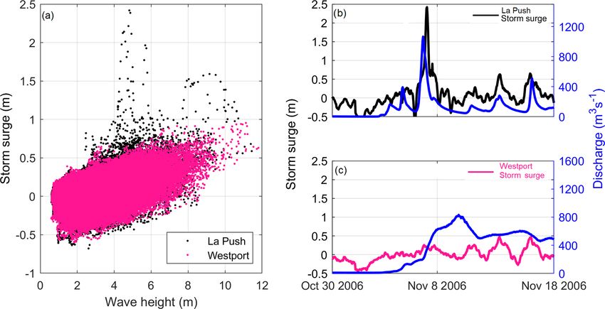
1418                                                                                      K. A. Serafin et al.: Competing processes

Figure 2. (a) The joint relationship between storm surge and wave height for La Push, Washington (black); and Westport, Washington (pink).
Example storm surge and discharge relationship at (b) La Push and (c) Westport, Washington.

complete, while the Calawah River is 99 % complete. An                    To further investigate the anomalously large ηSS at the
area scaling watershed analysis (Gianfagna et al., 2015) is            La Push tide gauge, the hydrodynamic model ADvanced
undertaken to rectify the discharge by the amount of un-               CIRCculation (ADCIRC, Luettich Jr. et al., 1992) and Simu-
gauged watershed. The watershed delineation shows that the             lating Waves Nearshore (SWAN, Zijlema, 2010) model (AD-
Bogachiel, Calawah, Sol Duc, and Dickey rivers account for             CSWAN; Dietrich et al., 2011) is used to simulate water
24 %, 22 %, 37 %, and 17 % of the total Quillayute River wa-           levels at the tide gauge during a storm event correspond-
tershed area, respectively. Noting the similar watershed char-         ing with the peak river discharge on record occurring on
acteristics and proportional watershed areas, the contribution         8 January 2009. ADCIRC is run in 2-D depth-integrated
of the Bogachiel River is estimated by scaling the Calawah             barotropic mode which performs well for calculating water
River discharge measurements by a factor of 2.09. This scal-           surface elevations during storm events (Weaver and Luet-
ing factor for estimating Bogachiel River discharge is val-            tich Jr., 2010). SWAN is run in nonstationary mode on an
idated by comparing to eight discharge point measurements              unstructured grid, allowing for tight coupling to ADCIRC.
taken during a US Geological Survey (USGS) survey in 2010              The model is run with two forcing implementations: one in-
(see Supplement). Discharge for the Quillayute River is es-            cluding a full forcing of waves, wind, pressure, streamflow,
timated by adding together discharge from the Sol Duc and              sea level anomalies, seasonality, and tides and one including
Bogachiel rivers.                                                      only streamflow and tides. Once the river-influenced water
   Hourly measured SWLs at the La Push tide gauge (NOAA                level is validated, it is removed from the ηSS signal and saved
station 9442396, 2004–2016) relative to Mean Lower Low                 as a sixth geophysical variable (ηRi ; see Supplement for re-
Water (MLLW) are downloaded, transformed into NAVD88,                  moval technique).
and decomposed into mean sea level (ηMSL ), tide (ηA ), and               Because of the short length of the La Push tide gauge
nontidal residual (ηNTR ). The ηNTR is further decomposed              record, decomposed water levels from the La Push tide gauge
into monthly mean sea level anomalies (ηMMSLA ), seasonal-             are merged with decomposed water levels from the Toke
ity (ηSE ), and storm surge (ηSS ), using methods described in         Point tide gauge (NOAA station 9440910) to create a com-
Serafin et al. (2017). Peak ηSS events at La Push are found            bined water level record with a length of 36 years. Details
to be the highest on record compared to all US west coast              of this methodology are explained in the corresponding Sup-
tide gauge stations (Serafin et al., 2017). Upon further in-           plement, as well as in Serafin et al. (2019). Once the two tide
vestigation of the ηSS record, a large portion of extreme              gauges are merged, the combined hourly tide gauge record
ηSS events occur during low-wave events (Fig. 2a) and high-            extends from 1980 to 2016 and is 97 % complete.
river-discharge events (Fig. 2b). This is inconsistent with ηSS
in Westport, Washington (Fig. 2a and c), just south of La
Push, and with other tide gauges along the US west coast (not
shown). It is therefore hypothesized that the anomalously
large signal seen in the ηSS is river-induced.

Nat. Hazards Earth Syst. Sci., 19, 1415–1431, 2019                              www.nat-hazards-earth-syst-sci.net/19/1415/2019/
K. A. Serafin et al.: Competing processes                                                                                       1419

4     Methods

Return level flood magnitudes, such as the 100-year event,
are typically assumed to be driven by a specific forcing event,
such as the 100-year rainfall or storm surge. However, for
processes driven by multiple dimensions, different sizes and
combinations of forcing conditions could potentially gener-
ate extreme flood magnitudes. To explore the role of com-
pounding forcings in generating extreme water levels, a hy-
brid modeling framework is developed by merging a hy-
draulic model simulating river flow with probabilistic simu-
lations of jointly occurring boundary conditions, in this case
SWL and river discharge (Fig. 3). Statistical simulations al-
low for long, synthetic records of joint forcings that may not
have occurred in the short observational records but are phys-
ically capable of co-occurring. Modeling all of the statisti-
cally simulated boundary conditions in a hydraulic model to
output along-river water levels would be prohibitively expen-
sive. As an alternative to time-consuming simulations, surro-
gate models (Razavi et al., 2012) are developed to approx-
imate the response of a hydraulic model simulation at each
along-river location. This technique allows for the analysis
of along-river water levels driven by a variety of boundary
conditions. Long synthetic records on the order of 500 years
allow for the direct empirical extraction of water level re-
turn levels rather than an extrapolation from historic observa-
tional forcing conditions. In addition, the large sample space
of simulated variables permits a comparison of event-based
return levels, where the 100-year water level is determined by
the 100-year forcing, to response-based return levels, where
                                                                   Figure 3. Schematic of hybrid statistical–physical modeling tech-
the 100-year water level is derived and then mapped to its
                                                                   nique. Models are portrayed as squares, while circles portray model
respective forcing conditions. This novel framework is flexi-      outputs.
ble for input of any statistical or hydraulic model. In this ap-
plication, we use the Serafin and Ruggiero (2014) full sim-
ulation total water level model and the US Army Corps of
Engineers’ (USACE) Hydrologic Engineering Center’s River           line. This technique is flexible to allow for both (i) the simu-
Analysis System (HEC-RAS; Brunner, 2016), which are de-            lation of the present-day climate for computing robust statis-
scribed in more detail below.                                      tics on extreme TWL events and (ii) the simulation of future
                                                                   climates and their impact on extreme TWLs. Because SR14
4.1    Probabilistic simulations of boundary conditions            was developed for use in open-coast environments, it does
                                                                   not include a procedure for simulating estimates of river dis-
The nonstationary, probabilistic simulation model of Serafin       charge, which is present in the local tide gauge at the La Push
and Ruggiero (2014) (hereinafter SR14) was developed to            study site. SR14 is therefore modified to produce synthetic
produce synthetic time series of daily maximum total water         time series of river discharge as well as a river-induced water
levels (TWLs), the combination of waves, tides, and nontidal       level.
residuals, on open-coast sandy beaches. SR14 simulates the            High-discharge events on the two gauged rivers in the wa-
individual components of the TWL in a Monte Carlo sense,           tershed, the Sol Duc and Calawah rivers, tend to occur within
while appropriately accounting for any dependencies exist-         hours of peak wave events recorded in offshore wave buoy
ing between the variables. This modeling technique is able         records and water level events recorded in the tide gauge
to include nonstationary processes influencing extreme and         data. Due to the interrelated nature of these forcings, daily
nonextreme events, such as seasonality, climate variability,       maximum estimates of Calawah River discharge (QC ) are
and trends in wave heights and water levels. SR14 outputs          compared to all variables simulated in the SR14 model (e.g.,
a number of synthetic records of all variables driving TWLs        wave height, ηSS , ηNTR , ηMMSLA ) to capture any dependen-
that produce alternate, but physically plausible, combinations     cies between these processes. The variable with the highest
of waves and water levels along an identified stretch of coast-    monthly correlation to QC is wave height (Hs ). Extreme QC

www.nat-hazards-earth-syst-sci.net/19/1415/2019/                          Nat. Hazards Earth Syst. Sci., 19, 1415–1431, 2019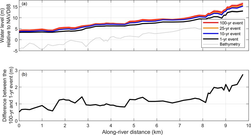
1420 K. A. Serafin et al.: Competing processes
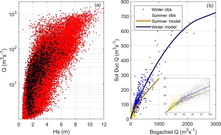
Figure 4. (a) Joint relationship between wave height (Hs ) and discharge (Q) for the observational record (black) and one example 500-year
simulation (red). (b) Seasonal model fit for the probabilistic simulation of the Sol Duc River Q in relation to the Bogachiel River Q. The
inset displays the model fits for discharge less than 100 m3 s−1 .
events are simulated using a bivariate logistic model, which For the winter season,
is the same technique used to simulate ηSS . The bivariate lo-
gistic model preserves the dependency and frequency of oc- QSD = 0.816QB + 1.168 (4)
currence of joint Hs − Q events in extreme and nonextreme
space. This technique generates a synthetic record of QC that is used when QB falls between 0 and 25 m3 s−1 , and
is seasonally varying, related to larger-scale climate variabil-
ity through wave height (essentially as a proxy for storms), QSD = −1.0 × 10⁻⁴ Q2B + 0.46QB + 16.11 (5)
and carries the same dependency between variables as the ob-
is used when QB falls between 25 and 2300 m3 s−1 (Fig. 4b).
servational record (Fig. 4a). QC is then multiplied by 2.09 to
When QB is greater than 2300 m3 s−1 , QSD is determined
represent inflow from both the Bogachiel and Calawah rivers.
using
Discharge measurements at the Sol Duc River are
highly correlated with the discharge measurements at the QSD = 0.075QB + 500.42. (6)
Calawah River (ρ = 0.9, τ = 0.83); thus Sol Duc River dis-
charge (QSD ) is modeled based on a relationship with the Summer and winter QB is binned and residuals of QSD from
scaled QC , representing the Bogachiel River (QB ). Estimates the above model fits are generated. Normal distributions are
of QSD are related to QB during the summer and winter sea- fit to QSD residuals in each bin, except for low bins (less
sons. First, daily maximum Q is split into summer (May, than 25 m3 s−1 ) where residuals are fit to exponential dis-
June, July, August, September, and October) and winter (Jan- tributions. QSD is then directly related to simulated esti-
uary, February, March, April, November, and December) mates of QB ; QSD is first determined by fitting the prescribed
seasons. Next, models are fit to the joint relationship between model to each estimate of QB , and then a random sample
the QSD and QB each season, such that for the summer sea- is taken from the residuals per binned QB and added to the
son, model. This technique captures the joint peaks of the river
QSD = 1.186QB + 0.226 (1) systems visible in the observed dataset, while allowing for
variability between the simulated estimates (Fig. 4b).
is used when QB falls between 0 and 10 m3 s−1 , and
4.1.1 Modeling the river-induced water level
QSD = −1.0 × 10⁻⁴ Q2B + 0.38QB + 14.07 (2)
is used when QB falls between 10 and 700 m3 s−1 (Fig. 4b). At tide gauges along the US west coast, the maximum daily
When QB is greater than 700 m3 s−1 , QSD is determined us- SWL generally occurs during, or close to, the daily high tide
ing (Serafin and Ruggiero, 2014; Serafin et al., 2017). Modeling
peaks in ηRi that occur during low tide would therefore erro-
QSD = 0.216QB + 61.25. (3) neously increase simulated estimates of the SWL occurring
Nat. Hazards Earth Syst. Sci., 19, 1415–1431, 2019 www.nat-hazards-earth-syst-sci.net/19/1415/2019/
K. A. Serafin et al.: Competing processes                                                                                              1421

Figure 5. (a) The relationship between the river-influenced water level (ηRi ) and Bogachiel River discharge on a log-linear scale. The solid
black line represents the model fit to the observational records (black dots). (b) The percentage of time ηRi occurs in the record during a
specific QB . In both panels, black represents the observational record and red represents one example 500-year simulation.

during high tide. Thus, instances of ηRi occurring approxi-              between 840 and 2090 m3 s−1 (Fig. 5b). For QB greater than
mately during high tide are retained and all other ηRi peaks             2090 m3 s−1 , ηRi occurs approximately 50 % of the time. The
are discarded, resulting in 155 ηRi events.                              frequency of occurrence of ηRi is modeled using a best-fit cu-
   Synthetic estimates of ηRi are developed by relating QB               bic function, where the frequency of occurrence is a function
and ηRi . This relationship is modeled using                             of QB based on the percentage of time the values have oc-
                                                                         curred in the record. Because there are no events greater than
ηRi = 0.039QB + 0.854 × 10⁻³                                    (7)      2500 m3 s−1 on record, we represent the percentage of occur-
                                                                         rence over this value as 100 % (Fig. 5b).
when QB is below 190 m3 s−1 and                                             Once QB is simulated using SR14, ηRi is simulated for
                                                                         every day in time by selecting the synthetic daily estimate
ηRi = 0.093QB + 0.284 × 10⁻³                                    (8)      of QB and randomly sampling from a normal distribution for
                                                                         each QB bin, where µ is the regression model and σ is the
when QB is above 190 m3 s−1 (Fig. 5a). Next, coarse bins
                                                                         standard deviation from each bin (Fig. 5a). The frequency-of-
ranging from 100 to 4000 m3 s−1 are created and the stan-
                                                                         occurrence model is then used to select the correct proportion
dard deviation (σ ) of ηRi within each bin is saved. For bins
                                                                         of ηRi events to retain for each synthetic simulation. These
that contain less than 10 observations, observations from the
                                                                         techniques capture both the spread of ηRi related to QB and
previous bins are included until there are more than 10 obser-
                                                                         the percentage of time of occurrence (Fig. 5).
vations per bin for σ calculations. Finally, a two-point run-
ning average is used to smooth σ from each bin to ensure
continuous transitions and to avoid the edge effects from bin-           4.2   Hydraulic model for along-river water levels
ning a sparse dataset.
   There are times of high QB without a distinguishable ηRi              While a variety of hydraulic models can be used for deter-
in the tide gauge record; thus a model is also developed to              mining the elevation of along-river water levels, we employ
simulate the frequency of occurrence of ηRi during daily                 the Hydraulic Engineering Center’s River Analysis System
maximum SWLs. The frequency of occurrence of ηRi is de-                  (Brunner, 2016). HEC-RAS is used to estimate water sur-
fined as the percentage of time ηRi occurs in the observa-               face elevations in rivers and streams in both steady and un-
tional record, which is less than 10 % of the time when QB is            steady flow and under subcritical, supercritical, and mixed
less than 840 m3 s−1 and 10 %–25 % of the time when QB is                flow regimes (Goodell, 2014). HEC-RAS has been previ-

www.nat-hazards-earth-syst-sci.net/19/1415/2019/                                Nat. Hazards Earth Syst. Sci., 19, 1415–1431, 2019
1422 K. A. Serafin et al.: Competing processes
Figure 6. Digital elevation model (DEM) used for the HEC-RAS simulations of the Quillayute River. HEC-RAS cross sections are depicted
as grey lines. Approximate river kilometer and the location of the tide gauge are depicted as diamonds and a square, respectively.
ously used to model water surfaces for a range of applications 4.3 Hybrid statistical–physical modeling
including, but not limited to, floodplain mapping (Yang et al.,
2006), flood forecasting (Saleh et al., 2017), dam breaching
The modified simulation technique of SR14 is used to
(Butt et al., 2013), and flood inundation (Horritt and Bates,
produce 70 500-year-long synthetic records representing
2002). HEC-RAS computes water levels by solving the 1-D
present-day climate for the time period of 1980–2016 of
energy equation with an iterative procedure, termed the step
daily maximum SWL and Q for both the Sol Duc and Bo-
method, from one cross section to the next (Brunner, 2016).
gachiel rivers. Rather than run the ∼ 13 million simulated
For subcritical flows, the step procedure is carried out mov-
conditions through a numerical model, a limited set of joint
ing upstream; computations begin at the downstream bound-
boundary conditions of SWL and Q (at the Bogachiel and Sol
ary of the river and the water surface elevation at an upstream
Duc rivers) are run through HEC-RAS, outputting the eleva-
cross section is iteratively estimated until a balanced water
tion of the along-river water level at each HEC-RAS transect.
surface is obtained. Energy losses between cross sections are
Surrogate models are generated from the HEC-RAS runs for
comprised of a frictional loss via the Manning equation and
each transect using a scattered linear interpolation of the 3-D
a contraction/expansion loss via a coefficient multiplied by
surface of boundary conditions. The number of combinations
the change in velocity head (see Brunner, 2016, for more de-
of SWL and Q used to develop the surrogate models are cho-
tails).
sen to minimize interpolation errors during validation runs.
In this application, HEC-RAS is used to model 1-D wa-
A daily estimate of water level elevation at each transect is
ter levels under gradually varied, steady-flow conditions at
produced by inputting all daily maximum SWL and Q con-
transects along the Quillayute River. While a simplification
ditions into the surrogate models, which efficiently extract
of flood processes, the 1-D application is commonly used
along-river water levels for any set of SWL and Q inputs.
to create flood hazard maps. A detailed digital elevation
Using the count-back method, where for example the fifth
model (DEM) is developed for the river network, includ-
largest event for each synthetic record would be the 100-year
ing bathymetry and topography for the floodplains of inter-
event, water level return levels are extracted for all 70 500-
est (Fig. 6). Model domain boundary conditions are chosen
year synthetic records for the (1) along-river water levels at
as the SWL at the tide gauge (m; downstream boundary)
each transect, (2) SWLs, and (3) Q. This methodology pro-
and river discharge from the Sol Duc and Bogachiel rivers
vides both an estimate of the return level magnitude (e.g.,
(m3 s−1 ; upstream boundary). The HEC-RAS model is val-
the average of the 70 100-year events) and the uncertainty
idated using water surface measurements from a 2010 sur-
around that magnitude (e.g., the distribution of the 70 100-
vey. Details of the HEC-RAS model validation and calibra-
year events). It also provides a technique to compare the
tion procedures are documented in the Supplement.
response-based return level (e.g., the 100-year water level)
Nat. Hazards Earth Syst. Sci., 19, 1415–1431, 2019 www.nat-hazards-earth-syst-sci.net/19/1415/2019/K. A. Serafin et al.: Competing processes 1423
5.2 Surrogate model validation
A number of validation scenarios are modeled in HEC-
RAS to determine whether the combinations of Q and SWL
boundary conditions used to develop the surrogate models
represent a large enough sample space of forcing conditions
for the interpolation of along-river water levels. The valida-
tion scenarios are chosen to cross through both HEC-RAS
modeled and unmodeled conditions (Fig. 8a). Across all vali-
dation scenarios, the average root mean square error (RMSE)
between the HEC-RAS directly modeled and the surrogate
model-interpolated water levels is 1 cm. Only 1.5 % of the
validation scenarios have a bias greater than 10 cm, and the
largest RMSE at any transect is 20 cm across all scenarios
(Fig. 9). The validation scenario with the worst performance
Figure 7. Resulting storm surge (a) and still water level (b) at the occurs during high QB and low QSD paired with low-SWL
La Push tide gauge modeled using ADCIRC for a simulation in- events. However, even during the worst-performing case,
cluding full forcing (red) and a simulation including only discharge the difference between the HEC-RAS directly modeled wa-
and tides (blue) compared to the observational record (black). The ter level and the surrogate model-interpolated water level is
ADCIRC simulation was run for the maximum discharge event on small (Fig. 8b). The main research focus here is extreme wa-
record occurring on 8 January 2009.
ter levels, and the conditions driving low-probability return
level events rarely fall around the scenarios with the highest
bias.
to the event-based return level (e.g., the water level driven by
the 100-year SWL or 100-year Q event). 5.3 Hybrid modeling of along-river water levels
5.3.1 Temporal variability
5 Results
Seasonal variability exists in the elevation of along-river
The following section first validates the presence of a river-
water levels. The highest elevation water level occurs dur-
induced water level within the tide gauge signal and then
ing the winter (here defined as December, January, Febru-
demonstrates the effectiveness of the surrogate models in
ary), while the lowest elevation water level occurs during
representing along-river water levels for unmodeled HEC-
the spring (March, April, May) (Fig. 10a). The spring along-
RAS boundary conditions. Next, the spatial and tempo-
river water level is on average 0.50 m lower than the winter
ral variability of the magnitude of along-river water lev-
along-river water level, 0.33 m lower than the fall (Septem-
els and their driving conditions are examined. Finally, low-
ber, October, November) along-river water level, and 0.03 m
probability water levels, like the 100-year event, are extracted
lower than the summer (June, July, August) along-river wa-
from the simulated records of along-river water levels, and
ter level (Fig. 10b). The difference between seasonal along-
the dominant drivers are evaluated.
river water levels is nonlinear upstream, and certain sections
5.1 River-induced water level validation of the river have larger changes in elevation between months
(Fig. 10b). However, this variation becomes relatively linear
Results from ADCSWAN modeling of the 8 January 2009 downstream of river kilometer 3.
storm event show that the simulation including only river The seasonal variability of the along-river water level is
discharge and tides is nearly able to recreate the measured driven by the seasonality of the forcings, which are well
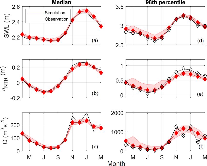
peak ηSS signal at the tide gauge (Fig. 7a). The addition of represented in the simulations compared to the observations
wind, pressure, waves, sea level anomalies, and seasonality is (Fig. 11). The monthly median SWLs and ηNTR ’s are higher
found to have minimal impact on the peak observed ηSS . Fur- in the winter than in the summer (Fig. 11a and b). This
thermore, the maximum ηSS occurs during low tide (Fig. 7b), cyclical variability is also depicted in the monthly median
which indicates a potential relationship between water sur- river discharge from the Quillayute River (combined Sol Duc
face elevation, tidal level, and river discharge. While the and Bogachiel Q) and is approximately 200 m3 s−1 higher in
ADCSWAN runs only explore one instance of this phe- winter months than summer months (Fig. 11c). The 98th per-
nomenon, it provides physics-based evidence that anoma- centile values of SWL, ηNTR , and Q have a similar seasonal
lously high ηSS at the La Push tide gauge is likely being variability to the median conditions (Fig. 11d–f).
driven by large discharge events.
www.nat-hazards-earth-syst-sci.net/19/1415/2019/ Nat. Hazards Earth Syst. Sci., 19, 1415–1431, 20191424 K. A. Serafin et al.: Competing processes
Figure 8. (a) Modeled HEC-RAS Q boundary conditions used to generate the surrogate models (red-dotted lines) compared to the simulated
conditions used for surrogate model validation (green dots). The black dots represent the observational daily max conditions, while the
colored circles represent the worst performing of the validation tests. The red and blue colored circles represent the scenarios where the
interpolated water surface had a bias of over 10 cm lower than the model. (b) Example along-river water level for the worst-performing
condition in the validation tests.
5.3.2 Spatial variability ter level event. Downstream 100-year water levels are driven
by SWLs, upstream 100-year water levels are driven by Q,
The large number of joint SWL and Q conditions allows for and the 100-year water level between kilometer 1 and 2 is
the direct extraction of water level return levels and the corre- driven by different combinations of high- and low-SWL and
sponding univariate or multivariate drivers along each HEC- Q events (Fig. 13b).
RAS transect. The magnitude of the 100, 25, 10, and annual The relative importance of both oceanic and riverine forc-
return level water levels is between 3 and 17 m (NAVD88, ing to extreme water levels emerges when averaging the mag-
Fig. 12a). While the peaks in return level events occur at nitude of the drivers of the water level return levels at each
similar locations, the difference between return level events transect from all 70 500-year-long simulations (Fig. 14). The
varies spatially moving upriver. For example, at river kilome- magnitude of the average Q driving water level return lev-
ter 1, the difference between the average (of all simulations) els gradually increases by approximately 1000 m3 s−1 over
annual and 100-year event is approximately 0.9 m, whereas river kilometer 0–2 and then is consistent from river kilome-
at river kilometer 8 and upstream, the difference between ter 2 to 10 (Fig. 14a). Downstream, between river kilometer 0
these two events is closer to 2 m (Fig. 12b). and 0.25, the magnitude of the average SWL driving water
The dominant forcing conditions driving water level return level return levels is consistent and then gradually decreases
levels vary along-river. At the river mouth, the annual water over a 1 km zone (Fig. 14b).
level event (e.g., the event that is expected every year) in each When comparing to water level return levels driven by a
simulation occurs during Q ranging from 40 to 2600 m3 s−1 univariate forcing or event return level (e.g., along-river wa-
and SWLs around 3.3 m, which corresponds with the annual ter levels modeled from the 100-year Q or SWL event), we
SWL event (Fig. 13a). Moving upstream to river kilometer 1 find that the stretches of river driven by a consistent SWL
and 2, the annual water level event is driven by both high or Q forcing approximate the univariate return level event.
SWL occurring during low Q and low SWL occurring dur- Therefore, the 100-year SWL does indeed cause the 100-year
ing high Q. At river kilometer 4, the annual water level event water level downstream, between river kilometer 0 and 0.25,
occurs during the annual Q event coincident with SWLs that while the 100-year Q event drives the 100-year water level
range from 1.8 to 3.9 m (Fig. 13a). These results are simi- upstream, between river kilometer 2 and 10 (dashed lines,
lar, albeit events are larger magnitude, for the 100-year wa- Fig. 14). However, between river kilometer 0.25 and 1.75 a
Nat. Hazards Earth Syst. Sci., 19, 1415–1431, 2019 www.nat-hazards-earth-syst-sci.net/19/1415/2019/K. A. Serafin et al.: Competing processes 1425
Figure 9. (a) Average root mean square error (RMSE) and (b) bias for all 197 discharge validation scenarios across 4 out of the 15 SWL
scenarios. The worst-performing model is discharge scenario 153.
flood transition zone is present, where neither the SWL re-
turn level or the Q return level events drive the water level
return level. This is consistent across all return level events.
6 Discussion
The hybrid model developed in this study, which combines
statistical simulations with a physics-based model, provides
an approach for probabilistically evaluating the conditions
that drive extreme water levels not only in an open-coast
setting, but also kilometers upriver. The ability to simulate
millions of combinations of Q and SWL events allows for a
robust estimate of resulting along-river water levels, which
numerical models alone are unable to consider due to large
computational expenses. While some of our modeling tech-
niques are specific to this location, the overall framework
Figure 10. (a) Variability of along-river water levels averaged for combining statistical and physics-based models is gen-
over spring (MAM), summer (JJA), fall (SON), and winter (DJF). eral enough for use in coastal locations throughout the globe
(b) The difference between the spring and summer, fall, and winter where flooding arises from compounding processes.
along-river water levels. The decomposition of the SWL into low- and high-
frequency signals, including a river-influenced component,
helps identify the importance of physical processes for gener-
ating high water levels across various regional settings. This
www.nat-hazards-earth-syst-sci.net/19/1415/2019/ Nat. Hazards Earth Syst. Sci., 19, 1415–1431, 20191426 K. A. Serafin et al.: Competing processes Figure 11. (a–c) Observational (black) and simulated (red) monthly median still water level (SWL), nontidal residual (etaNTR ), and dis- charge (Q). (d–f) Observational (black) and simulated (red) monthly 98th percentile of the SWL, ηNTR , and Q. Red shading indicates the bound from each simulation. Figure 12. (a) The water level return level at each transect for all 70 probabilistic simulations. Each return level event displays the average of the simulations (solid line) as well as the range around the average (shaded). (b) The along-river difference between the annual and 100-year event, averaged over 70 simulations. is especially important in locations like the US west coast, discharging directly into the ocean. This is dissimilar to other where the steep, narrow continental shelf prevents wind- tide gauges in the region which are located in larger estuar- and pressure-driven storm surge from being overwhelmingly ies, situated away from river input. Estuaries typically exhibit large (Allan et al., 2011). The influence of the river signal in wave, tide, or river-dominant morphology, based on the rel- the tide gauge is directly related to the setting of our study ative energy of each process (Dalrymple et al., 1992). The site. The estuary is relatively small and narrow with the river Quillayute River outlets directly to a high-wave-energy en- Nat. Hazards Earth Syst. Sci., 19, 1415–1431, 2019 www.nat-hazards-earth-syst-sci.net/19/1415/2019/
K. A. Serafin et al.: Competing processes                                                                                              1427

Figure 13. The individual Q or SWL condition driving the (a) annual and (b) 100-year water level event at specific along-river locations for
each 70 500-year simulation. In both figures, the black lines represent the annual and 100-year return level magnitude for Q and SWL.

Figure 14. The average forcing condition driving along-river return levels at each transect where (a) displays the Quillayute Q conditions
and (b) displays the SWL conditions. The dashed lines depict the univariate forcing conditions, where the along-river return level is assumed
to be driven by either Q or SWL. Red, orange, blue, and black lines represent the 100, 25, 10, and annual return level event. The grey shaded
area represents a transition zone, where the water level is driven by a combination of SWL and Q events.

vironment and has a small estuary volume compared to its                 large estuary volume compared to river discharge are less in-
river input volume. The steep catchment of the mountain-                 fluenced by fluvial processes. Furthermore, a larger estuary
ous environment means a short response time for rainfall,                may experience variability in the water surface elevation due
therefore producing peak discharges temporally similar to                to wave-induced setup and/or other local storm-induced pro-
peak storm-induced still water levels, allowing for interac-             cesses (Cheng et al., 2014; Olabarrieta et al., 2011), which
tion between the two. In contrast, water level elevations with           may further dampen the influence of a river signal.

www.nat-hazards-earth-syst-sci.net/19/1415/2019/                                Nat. Hazards Earth Syst. Sci., 19, 1415–1431, 2019
1428                                                                                 K. A. Serafin et al.: Competing processes

   This research confirms the presence of an oceanographic–        of high-Q events along the Quillayute River. While we have
fluvial transition zone, where traditional, univariate method-     characterized the spatial variability in extreme water levels
ologies for defining return level events are insufficient for      in the present day, there is a high likelihood changes in the
defining water level return levels. Between river kilometer 1      future climate will shift the importance of these interacting
and 2, we find that a range of SWL and Q conditions drive          processes.
all return level events, and water levels are driven by nei-
ther the univariate SWL or Q return level event. A similar
flood zone transition was recently modeled numerically and,        7   Conclusions
albeit for a single event, physically demonstrates the impor-
                                                                   This research illustrates the importance of considering a large
tance of including multiple variables to reproduce accurate
                                                                   number of forcing conditions to model compounding pro-
flooding (Bilskie and Hagen, 2018). Thus, flood hazard as-
                                                                   cesses when evaluating extreme water levels. Here we find
sessments on systems with multivariate forcings may mis-
                                                                   that, in coastal settings, river discharge can be an important
represent water level elevations for low-probability events if
                                                                   driver of high water levels measured in a tide gauge. We also
only univariate variables are modeled. This has large implica-
                                                                   find that the univariate, event-based return level event, like
tions for characterizing the risk to flooding, especially in the
                                                                   the 100-year discharge, does not always match the response-
context of mapping flooding hazards. Furthermore, we show
                                                                   based return level, like the 100-year water level. Further-
that return level water levels can occur over a range of com-
                                                                   more, when processes compound, along-river return levels
bined extreme and nonextreme forcing in the flood transition
                                                                   may be driven by events that are not considered extreme
zone. This illustrates that, in order to properly understand
                                                                   themselves. Probabilistic techniques allowing for the anal-
the impacts of compounding flooding, more than just design
                                                                   ysis of thousands to millions of combinations of events not
scenarios need to be considered for the proper assessment of
                                                                   captured in the observational record provide a characteriza-
risk.
                                                                   tion of where river, ocean, or the combination of the two may
   Many of our results can be explained by dynamics that
                                                                   be important for generating extreme events.
occur during interacting ocean and river flows. For exam-
                                                                      Overall, the hybrid merging of a statistical and numeri-
ple, a coincidence of high SWL and peak river discharge
                                                                   cal model provides a methodology for better understanding
may induce blocking, where river-induced water levels are
                                                                   the drivers of flooding along the length of a river. While our
trapped upstream and either flood overbank or outlet to the
                                                                   model does not actively resolve the physical interaction of
ocean as the tide recedes (Kumbier et al., 2018; Chen and
                                                                   river and oceanographic flow, it develops an approach for
Liu, 2014). The outletting to the ocean as the tide recedes
                                                                   characterizing and extracting river-influenced water levels
artificially inflates SWLs at the tide gauge, increasing water
                                                                   measured at tide gauges while robustly modeling the drivers
levels for days at a time and prolonging exposure to flood-
                                                                   of extreme along-river water levels. Understanding the dom-
ing. When subtracting a tide time series from this signal,
                                                                   inant, spatially variable drivers of flooding events will help
storm surge would appear to be elevated at low tide. While
                                                                   coastal communities better understand their risks, which is
the ADCSWAN simulation confirms the presence of this ef-
                                                                   important for increasing resilience to future events.
fect by matching the peak storm surge at low tide, our hybrid
methodology only models steady-flow scenarios. Thus, with
co-occurring daily maximum SWL and discharge, our model
                                                                   Data availability. Data can be made available by the authors upon
may miss certain dynamics important for flooding over un-          request.
steady conditions. Furthermore, interactions between storm
surge and river discharge may increase the overall elevation
of the residual (Maskell et al., 2013). While beyond the scope     Supplement. The supplement related to this article is available
of our present study, these unsteady characteristics are impor-    online at: https://doi.org/10.5194/nhess-19-1415-2019-supplement.
tant to consider in future research.
   Because sea level rise, along with other changes to the
climate, will exacerbate the compounding effects of flood          Author contributions. The study and methodology were conceived
drivers (Moftakhari et al., 2017; Wahl et al., 2015), it is        by KAS and PR. KAS carried out the analyses, produced the results,
also important to consider the impact of changes to pro-           and wrote the manuscript under the supervision of PR. KP carried
cesses driving flooding events in the future (Zscheischler         out the analyses and produced the results of the ADCIRC simula-
et al., 2018). By 2100, the likely range of relative sea level     tions. KP also developed the topography/bathymetry DEM as well
rise in the La Push area is projected to be between 18 and         as the geometric files for use in HEC-RAS. KAS, PR, KP, and
                                                                   DFH all contributed by generating ideas, discussing results, and
80 cm, considering vertical land motion and various emis-
                                                                   editing the manuscript.
sions scenarios (Miller et al., 2018). The western Olympic
Peninsula is projected to experience increased winter pre-
cipitation (Mote et al., 2013; Halofsky et al., 2011), which
could subsequently increase either the frequency or intensity

Nat. Hazards Earth Syst. Sci., 19, 1415–1431, 2019                         www.nat-hazards-earth-syst-sci.net/19/1415/2019/
K. A. Serafin et al.: Competing processes 1429
Competing interests. The authors declare that they have no conflict and Mississippi. Part I: Model development and validation, Mon.
of interest. Weather Rev., 138, 345–377, 2010.
Butt, M. J., Umar, M., and Qamar, R.: Landslide dam and sub-
sequent dam-break flood estimation using HEC-RAS model in
Acknowledgements. Tide gauge records are available through the Northern Pakistan, Nat. Hazards, 65, 241–254, 2013.
National Oceanic and Atmospheric Administration (NOAA) Na- Chelton, D. B. and Enfield, D. B.: Ocean signals in tide gauge
tional Ocean Service (NOS) website, and river discharge is available records, J. Geophys. Res.-Solid, 91, 9081–9098, 1986.
through the US Geological Survey (USGS) National Water Infor- Chen, W.-B. and Liu, W.-C.: Modeling flood inundation induced by
mation System (https://waterdata.usgs.gov/wa/nwis/rt, last access: river flow and storm surges over a river basin, Water, 6, 3182–
October 2017). Bathymetric and topographic data for DEM cre- 3199, 2014.
ation were obtained from NOAA’s elevation data viewer. Thank you Cheng, T., Hill, D., and Read, W.: The Contributions to Storm Tides
to Michael Rossotto and Garrett Rasmussen for providing updated in Pacific Northwest Estuaries: Tillamook Bay, Oregon, and the
shapefiles of the Quileute Reservation boundaries. Thank you also December 2007 Storm, J. Coast. Res., 31, 723–734, 2014.
to two anonymous reviewers whose comments improved the qual- Couasnon, A., Sebastian, A., and Morales-Nápoles, O.: A Copula-
ity of this paper. This work was funded by the NOAA Regional In- Based Bayesian Network for Modeling Compound Flood Hazard
tegrated Sciences and Assessments Program (NA15OAR4310145) from Riverine and Coastal Interactions at the Catchment Scale:
and a contracted grant with the Quinault Treaty Area (QTA) An Application to the Houston Ship Channel, Texas, Water, 10,
tribal governments (Quinault Indian Nation, Hoh Indian Tribe, and 1190, https://doi.org/10.3390/w10091190, 2018.
Quileute Tribe). Czuba, J. A., Barnas, C. R., McKenna, T. E., Justin, G. B., and
Payne, K. L.: Bathymetric and streamflow data for the Quil-
layute, Dickey, and Bogachiel Rivers, Clallam County, Washing-
Financial support. This research has been supported by the NOAA ton, April–May 2010, in: vol. 537, US Department of the Interior,
Regional Integrated Sciences and Assessments Program (grant US Geological Survey, Reston, Virginia, 2010.
no. NA15OAR4310145). Dalrymple, R. W., Zaitlin, B. A., and Boyd, R.: Estuar-
ine facies models: conceptual basis and stratigraphic
implications: perspective, J. Sediment. Res., 62, 1130–
1146, https://doi.org/10.1306/D4267A69-2B26-11D7-
Review statement. This paper was edited by Paolo Tarolli and re-
8648000102C1865D, 1992.
viewed by Philip Ward and one anonymous referee.
de Vries, H., Breton, M., de Mulder, T., Krestenitis, Y., Ozer,
J., Proctor, R., Ruddick, K., Salomon, J. C., and Voor-
rips, A.: A comparison of 2D storm surge models applied
References to three shallow European seas, Environ. Softw., 10, 23–42,
https://doi.org/10.1016/0266-9838(95)00003-4, 1995.
Allan, J. C. and Komar, P. D.: Extreme storms on the Pacific North- Dietrich, J., Zijlema, M., Westerink, J., Holthuijsen, L., Dawson,
west coast during the 1997–98 El Niño and 1998–99 La Niña, J. C., Luettich Jr, R., Jensen, R., Smith, J., Stelling, G., and Stone,
Coast. Res., 18, 175–193, 2002. G.: Modeling hurricane waves and storm surge using integrally-
Allan, J. C., Komar, P. D., and Ruggiero, P.: Storm Surge Magni- coupled, scalable computations, Coast. Eng., 58, 45–65, 2011.
tudes and Frequency on the Central Oregon Coast, in: Proc. So- Gianfagna, C. C., Johnson, C. E., Chandler, D. G., and Hofmann,
lutions to Coastal Disasters Conf., 26–29 June 2011, Anchorage, C.: Watershed area ratio accurately predicts daily streamflow in
Alaska, 2011. nested catchments in the Catskills, New York, J. Hydrol.: Reg.
Bevacqua, E., Maraun, D., Hobæk Haff, I., Widmann, M., Stud., 4, 583–594, 2015.
and Vrac, M.: Multivariate statistical modelling of compound Goodell, C.: Breaking the HEC-RAS Code: A User’s Guide to Au-
events via pair-copula constructions: analysis of floods in tomating HEC-RAS, h2ls, Portland, OR, 2014.
Ravenna (Italy), Hydrol. Earth Syst. Sci., 21, 2701–2723, Graham, N. E. and Diaz, H. F.: Evidence for intensification of North
https://doi.org/10.5194/hess-21-2701-2017, 2017. Pacific winter cyclones since 1948, B. Am. Meteorol. Soc., 82,
Bilskie, M. and Hagen, S.: Defining Flood Zone Transitions in Low- 1869–1893, 2001.
Gradient Coastal Regions, Geophys. Res. Lett., 45, 2761–2770, Halofsky, J. E., Peterson, D. L., O’Halloran, K. A., and Hoffman,
2018. C. H.: Adapting to climate change at Olympic National Forest
Bromirski, P. D., Flick, R. E., and Miller, A. J.: Storm surge along and Olympic National Park, Gen. Tech. Rep. PNW-GTR-844,
the Pacific coast of North America, J. Geophys. Res.-Oceans, US Department of Agriculture, Forest Service, Pacific Northwest
122, 441–457, 2017. Research Station, Portland, OR, p. 130, 2011.
Brunner, G. W.: HEC-RAS River Analysis System Hydraulic Ref- Horritt, M. and Bates, P.: Evaluation of 1D and 2D numerical mod-
erence Manual, Version 5.0, Tech. rep., US Army Corps of En- els for predicting river flood inundation, J. Hydrol., 268, 87–99,
gineers, Institute for Water Resources, Hydrologic Engineering 2002.
Center, Davis, CA, 2016. Horsburgh, K. and Wilson, C.: Tide-surge interaction and its role in
Bunya, S., Dietrich, J. C., Westerink, J., Ebersole, B., Smith, J., the distribution of surge residuals in the North Sea, J. Geophys.
Atkinson, J., Jensen, R., Resio, D., Luettich, R., Dawson, C., Res.-Oceans, 112, 1–13, https://doi.org/10.1029/2006JC004033,
Cardone, V. J., Cox, A. T., Powell, M. D., Westerink, H. J., 2007.
and Roberts, H. J.: A high-resolution coupled riverine flow, tide,
wind, wind wave, and storm surge model for southern Louisiana
www.nat-hazards-earth-syst-sci.net/19/1415/2019/ Nat. Hazards Earth Syst. Sci., 19, 1415–1431, 2019You can also read