Incorporating the logistic regression into a decision-centric assessment of climate change impacts on a complex river system - HESS
←
→
Page content transcription
If your browser does not render page correctly, please read the page content below
Hydrol. Earth Syst. Sci., 23, 1145–1162, 2019
https://doi.org/10.5194/hess-23-1145-2019
© Author(s) 2019. This work is distributed under
the Creative Commons Attribution 4.0 License.

Incorporating the logistic regression into a decision-centric
assessment of climate change impacts on a complex river system
Daeha Kim1 , Jong Ahn Chun1 , and Si Jung Choi2
1 APEC    Climate Center, Busan, 48058, South Korea
2 Korea   Institute of Civil Engineering and Building Technology, Gyeonggi-do, 10223, South Korea

Correspondence: Si Jung Choi (sjchoi@kict.re.kr)

Received: 24 April 2018 – Discussion started: 18 May 2018
Revised: 13 February 2019 – Accepted: 20 February 2019 – Published: 28 February 2019

Abstract. Climate change is a global stressor that can un-        globe to sustain human livelihood and activities, those assets
dermine water management policies developed with the as-          have been traditionally managed by heuristic operation poli-
sumption of stationary climate. While the response-surface-       cies developed under the assumption of stationary climate
based assessments provided a new paradigm for formulat-           (Cosgrove and Loucks, 2015; Cully et al., 2016). However,
ing actionable adaptive solutions, the uncertainty associated     probabilistic behaviors of hydrological processes can be sig-
with the stress tests poses challenges. To address the risks of   nificantly altered by the warming atmosphere; therefore, the
unsatisfactory performances in a climate domain, this study       heuristic policies are expected to become increasingly vul-
proposed the incorporation of the logistic regression into a      nerable (Brown et al., 2015; Georgakakos et al., 2012).
decision-centric framework. The proposed approach replaces           When formulating management solutions to non-
the “response surfaces” of the performance metrics typically      stationary climate for a water system, an essential step is
used for the decision-scaling framework with the “logistic        to assess impacts of climate change on its performance.
surfaces” that describes the risk of system failures against      An established method for the impact assessment was to
predefined performance thresholds. As a case study, water         investigate outputs of relevant system models forced by
supply and environmental reliabilities were assessed within       projections of the general circulation models (GCMs) under
the eco-engineering decision-scaling framework for a com-         hypothetical greenhouse gas (GHG) emission scenarios
plex river basin in South Korea. Results showed that human-       (e.g., Xu et al., 2015; Eum and Simonovic, 2010). This
demand-only operations in the river basin could result in the     type of assessments takes the “predict-then-act” paradigm
water deficiency at a location requiring environmental flows.     for which the first prerequisite is sufficiently reliable pre-
To reduce the environmental risks, the stakeholders could         dictions. The GCM projections, however, are often biased
accept increasing risks of unsatisfactory water supply per-       by inappropriate model formulations and/or imperfectly
formance at the sub-basins with small water demands. This         understood physical processes (Stevens and Bony, 2013;
study suggests that the logistic surfaces could provide a com-    Deser et al., 2012; Dufresne and Bony, 2008; Stainforth et
putational efficiency to measure system robustness to cli-        al., 2005). Thus, they may contain unacceptable risk costs
matic changes from multiple perspectives together with the        for policymakers (Brown et al., 2012), hindering utilization
risk information for decision-making processes.                   of GCM-led strategies (Weaver et al., 2013; Brown and
                                                                  Wilby, 2012).
                                                                     To overcome the weakness of GCM-driven assessments
                                                                  in practical decision support, alternative frameworks within
1   Introduction                                                  the “robust decision” paradigm have emerged (e.g., Hadka et
                                                                  al., 2015; Whateley et al., 2014; Lampert and Groves, 2010).
Climate change is a global stressor that poses prodigious         These decision-centric approaches seek robust solutions that
challenges to long-term management of water resources.            can minimize adverse effects of climatic stresses on given
While water infrastructures have been constructed across the

Published by Copernicus Publications on behalf of the European Geosciences Union.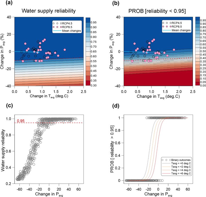
1146                         D. Kim et al.: Incorporating the logistic regression into a decision-centric impact assessment

hydrological systems. Examples include the decision scaling        isfactory performance on the response surface, the system of
(Brown et al., 2012), the dynamic adaptive policy pathways         interest could still be subject to a considerable risk of unsat-
(Haasnoot et al., 2013), the real option analysis (Woodward        isfactory performance.
et al., 2014), the info-gap decision theory (Korteling et al.,        Due to the associated uncertainty, the response surface of
2013), and the robust decision-making (Lampert and Groves,         general system performance needs to be treated in a proba-
2010), among others. Whereas the predict-then-act paradigm         bilistic manner. A possible approach is to gauge the uncer-
focuses on the most likely future conditions that can max-         tainty via the Monte Carlo sampling of system performances
imize expected utility, the decision-centric approaches pay        per climate stress (e.g., Steinschneider et al., 2015b; Whate-
attention to sensitivity (or vulnerability) of system perfor-      ley and Brown, 2016). However, if a complex system model
mance to climatic stressors (Weaver et al., 2013; Brown et         is employed with a large combination of climate stressors,
al., 2012). This paradigm accepts the irreducible uncertainty      this stochastic sampling approach would require expensive
in climate predictions as an inevitable part of long-term plan-    computational costs, even with modern computing power
ning and guides decision makers toward low-regret strategies       (Whateley et al., 2016). To explore the effect of internal cli-
for sustainable system performance under non-stationary cli-       mate variability with the exhaustive Monte Carlo sampling,
mate.                                                              the computational burden for the stress test would be multi-
   Among the decision-centric frameworks, the assessments          plied many times.
based on the response functions of system performance                 In this work, therefore, an efficient approach was proposed
have provided convenience in defining decision thresholds at       to evaluate the risks of system failures within a decision-
which adaptation actions are required (e.g., Kim et al., 2018;     centric framework. We simply incorporated the logistic re-
Steinschneider et al., 2015a; Turner et al., 2014; Whateley        gression into typical stress tests for the response-surface-
et al., 2014; Brown et al., 2012; Prudhomme et al., 2010).         based assessments. This study shows that the response sur-
They developed the relationships between system perfor-            face can be simply converted into a probabilistic domain by
mances and climatic stressors (hereafter referred to as the        categorizing the performance samples from the stress tests
response surfaces) via stress tests. Then, GCM projections         against a threshold. As a case study, we provided here a
were employed to indicate future system performance on             slightly modified version of the eco-engineering decision-
the response surfaces. The response-surface-based methods          scaling framework (Poff et al., 2016) to explore the probabil-
have been refined to consider spatially varying system per-        ities of system failures varying across a complex river system
formance (e.g., Schlef et al., 2018) and multiple management       with two contrasting management purposes.
objectives within a hydrological system (e.g., Culley et al.,
2016). They allowed efficient evaluation of climate change
risks by simply comparing the performance metrics indicated        2     Methodology
by a collection of GCMs against predefined thresholds.
   Nonetheless, uncertainty of the response surfaces can-          2.1    Eco-engineering decision-scaling framework
not be neglected due to assumptions and simplifications as-
sociated with the stress tests. Kim et al. (2018), for in-         The eco-engineering decision-scaling (EEDS) framework
stance, showed how climate change risks could be underes-          (Poff et al., 2016) expanded the decision scaling (Brown et
timated if a modeling scale was inappropriately chosen. Kay        al., 2012) to consider stakeholders’ multifaceted interests in
et al. (2014) emphasized the importance of uncertainty al-         the response surfaces. Five iterative steps are required for
lowances being used alongside the response surfaces. More-         this framework. Step 1 is to identify possible management
over, Steinschneider et al. (2015b) suggested that hydrolog-       options (e.g., upgrading operations and/or structural invest-
ical modeling and climatic variability may introduce uncer-        ments), to select indicators of ecological and engineering
tainty in the response surfaces as much as GCM projections.        performances (e.g., water supply reliability and ecological
The prior studies imply that over-reliance on the response         vulnerability), and to define user-specific thresholds under
surfaces of general performance metrics may misguide users         which the system performs unacceptably. Step 2 is to build
to inappropriate and/or untimely adaptation policies. Impor-       system models for the hypothetical stress tests. For water re-
tantly, the response surfaces have usually been developed          source management, the system models may include a runoff
with climatic shifts defined by long-term changes in statisti-     model and a water allocation model. By exposing the system
cal moments of weather observations (e.g., Poff et al., 2016;      models to a wide range of hypothetical climatic stressors,
Steinschneider et al., 2015a; Whateley et al., 2014; Turner        ecological and engineering performances can be evaluated.
et al., 2014), even though they might insufficiently explain       In step 3, the response surfaces of engineering and ecologi-
variation in the chosen performance indicators. Whateley and       cal performances are developed with outcomes of the stress
Brown (2016) found that the performance variation in a water       tests. For vulnerability analysis, the predefined thresholds are
supply system can be attributed significantly to the internal      imposed on the response surfaces. Step 4 is to evaluate the
climate variability over a time horizon of policy planning. In     management options with the size of the climatic zones sat-
other words, even if a projected climatic shift indicates a sat-   isfying the performance thresholds. In step 5, preferred de-

Hydrol. Earth Syst. Sci., 23, 1145–1162, 2019                                    www.hydrol-earth-syst-sci.net/23/1145/2019/

D. Kim et al.: Incorporating the logistic regression into a decision-centric impact assessment                               1147

cisions for the management options can be made, or, if nec-        9915 km2 (Fig. 1). The mean and the highest elevations in
essary, the assessment from step 1 to 4 can be repeated with       the river basin are 85 m and 1596 m a.s.l. (above sea level),
new management options and/or different criteria.                  respectively. The mean basin slope is 16.7 %. The total length
   In the EEDS framework, the key information would be the         of the main channel is approximately 402 km. The river basin
size of the climate zone mutually satisfying the engineering       has a semi-humid climate with monsoonal summer seasons.
and ecological thresholds since it measures overall system         Wet air masses moving from the North Pacific usually make
robustness to climate stresses. Decision makers may prefer         for hot and humid summer seasons, whereas winter seasons
management options that can widen the mutual climate zone,         are dry and cold due to the Siberian high pressure. Approx-
if they are socio-economically viable. However, the system         imately 60 %–70 % of annual precipitation falls in June to
robustness is not the only criterion for selecting manage-         September (KMA, 2011); thus, rivers flow across the basin
ment options. In decision-making processes, questions can          peaks in the middle of summer monsoon seasons. Snowmelt
be raised such as “what if future climates will not fall within    runoff minimally contributes to streamflow variations due to
the mutual climate zone?” and “how much do risks of system         small winter precipitation (Bae et al., 2008).
failures still exist within the climate zone that expects satis-      The Geum River basin is officially divided into 14 sub-
factory performances?” Those questions can be answered by          basins for administrative purposes along the geomorpholog-
incorporating the logistic regression and a collection of GCM      ical boundaries. The sub-basin areas vary between 120 and
projections into the EEDS framework.                               1856 km2 , with an average of 708 km2 . 60 % of the entire
                                                                   river basin is covered by forests, while agricultural areas
2.2    Incorporating the logistic regression into the stress       account for 18 %. The forest covers and agricultural lands
       tests                                                       within the 14 sub-basins occupy 33 %–83 % and 4.6–42 %,
                                                                   respectively. The sub-basins with relatively large agricultural
The stress tests in step 3 for the EEDS framework are in-          lands tend to have small forest covers. The urban areas are
tended to find expected performances per given climate expo-       5.3 % of the river basin in total. According to the Korea For-
sure. By comparing the obtained performances against a pre-        est Service (http://forest.go.kr, last access: 11 October 2017),
defined threshold, the climate exposures applied to the stress     the soils across the Geum River basin have moderate to high
tests can be categorized into binary outcomes (i.e., 1 for sat-    infiltration capacity, implying that sub-surface runoff gener-
isfactory performances and 0 for other cases). With no need        ations are dominant.
for the homogeneity and normality assumptions, the logistic           Human intervention affects the flow regimes in the Geum
regression model allows the explanation of occurrences of          River basin. The main channel is regulated by two large dams
the satisfactory performances with the sigmoid function of         serially connected for water supplies and flood controls. The
the climate exposures (xi ):                                       Yongdam Dam located in the upper river basin has an ef-
                        1                                          fective storage capacity of 809 Mm3 , while the Daecheong
π=                                              ,           (1)    Dam at the middle of the main channel has a larger capacity
       1 + exp [− (β0 + β1 x1 + β2 x2 + · · ·)]
                                                                   of 1040 Mm3 . Water storage in both dams is delivered to sev-
where π is the probability of satisfactory performance and         eral sub-basins through water distribution systems developed
βi is the regression coefficients. Thus, 1 − π becomes the         for municipal and industrial (M & I) water demands, making
probability of unsatisfactory performance.                         non-geomorphological human-made connectivity between
   When two explanatory variables are chosen for xi (e.g.,         the sub-basins. The two large dams supply water to the de-
changes in mean annual precipitation and temperature), it          mand sectors in outsides of the river basin through the distri-
is possible to develop a two-dimensional surface to describe       bution systems; hence, inter-basin water transfers may con-
variation in π within a climate domain. Hereafter, the surface     flict with water demands within the river basin. During mon-
of π will be referred to as the logistic surface. In this study,   soon seasons, the Yongdam and Daecheong dams should re-
the logistic surfaces were used for the steps 3 and 4 of the       duce their storage limits by 137 and 250 Mm3 for flood con-
EEDS framework in lieu of the response surfaces. The fol-          trol, respectively. In addition, many small-sized local reser-
lowing example shows how to assess the risk of system fail-        voirs are widespread across the river basin to sustain irrigated
ures together with robustness to climate stresses for a com-       agriculture (mostly for planting paddy rice). Though 95 %
plex water system.                                                 of the small reservoirs have minimal storage capacities be-
                                                                   low 1 Mm3 , their gross capacity is more than 320 Mm3 and
3     Application: a case study for optimal water                  thus considerably alters natural flow regimes. The total stor-
      allocation in a complex water system                         age capacities of the agricultural reservoirs in the 14 sub-
                                                                   basins are from 1.1 to 100.9 Mm3 , with a median value of
3.1    Study area                                                  12.5 Mm3 . In each sub-basin, natural river flows and water
                                                                   transferred from the storage facilities (i.e., the agricultural
The case study area is the Geum River basin located in the         reservoirs and dams) are consumed for agricultural, munici-
western–central part of South Korea with a total area of           pal, and industrial purposes. The water diverted for the M & I

www.hydrol-earth-syst-sci.net/23/1145/2019/                                     Hydrol. Earth Syst. Sci., 23, 1145–1162, 2019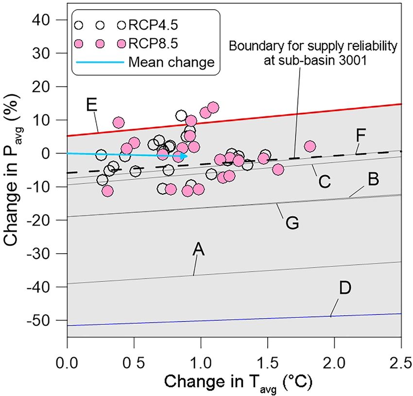
1148 D. Kim et al.: Incorporating the logistic regression into a decision-centric impact assessment
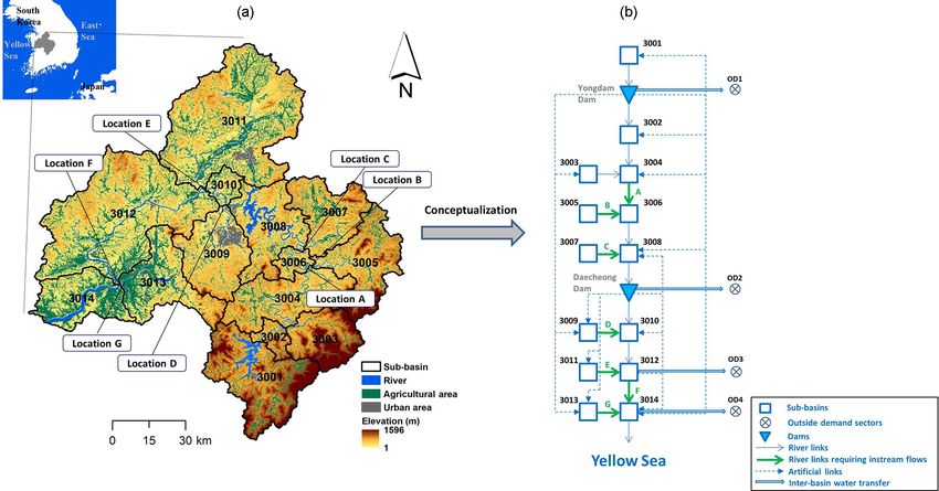
Figure 1. Layout of the Geum River basins (a) and the simplified node-and-link network for modeling water allocations (b).
demands could return to the rivers, becoming available water al., 2008), and overestimated values were smoothed by the
for lower demand sectors. inverse distance method. Jung and Eum (2015) found im-
For water allocation modeling, we simplified the complex proved performance of the combined method in South Ko-
river system with a node-and-link network shown in Fig. 1. rea via comparative evaluations to the original PRISM. For
Each sub-basin was conceptualized as a node with natural the case study, the collected grid data were spatially aggre-
water availability (i.e., natural runoff), storage capacity (i.e., gated with the sub-basin boundaries. The aggregated daily
water storage in the agricultural reservoirs), and water de- precipitation and temperature were perturbed by a stochastic
mands (i.e., agricultural and M & I water uses). The sub- weather generator for the stress tests and were then used to
basin nodes were connected by the stream links (the con- generate streamflow at the sub-basin nodes. According to the
tinuous lines). The two large dams were represented by the grid data, the mean annual precipitation and temperature over
nodes only having storage capacities and were located be- the Geum River basin for 1976–1995 were 1245 mm and
tween the two adjacent sub-basins accordingly. The outside 11.7 ◦ C, respectively. They have risen to 1325 mm (+6.4 %)
water demand sectors were represented by nodes with no nat- and 12.2 ◦ C (+0.5 ◦ C) during 1996–2015, providing an indi-
ural flows and zero storage capacities. The human-made con- cation that atmospheric water supply and demand gradually
nections between the dams and the sub-basins were concep- increase over time within the river basin.
tualized by separate links (the dashed lines) with conveyance The water demands for 2030 were taken as the reference
limits. demands to evaluate water allocation performance across
the river basin. In South Korea, government-driven national
3.2 Data collections water resources plans are legally developed for sustainable
resource management for every 20-year period. The wa-
3.2.1 Climate and water demand data ter resources plan for 2020 was first established in 2000
including water demand projections up to 2020 (MOCT,
We collected daily precipitation and maximum and mini-
2000) and has been revised three times to consider hydro-
mum temperatures over South Korea at 3 km grid resolu-
logic and socio-economic changes since the initial version
tion for 1973–2015. The grid data were produced by in-
(MOCT, 2006; MLTM, 2011; MOLIT, 2016). In the third
terpolating synoptic observations at 60 stations in the auto-
version of the water resources plan for 2020 (MOLIT, 2016),
mated surface observing system (ASOS) operated by the Ko-
the water demands across South Korea were re-projected
rea Meteorological Administration. The point weather data
up to 2030. By an electronic correspondence (requested on
were spatially interpolated by the parameter-elevation re-
26 September 2017), we obtained the demand data projected
gressions on independent slopes model (PRISM; Daly et
Hydrol. Earth Syst. Sci., 23, 1145–1162, 2019 www.hydrol-earth-syst-sci.net/23/1145/2019/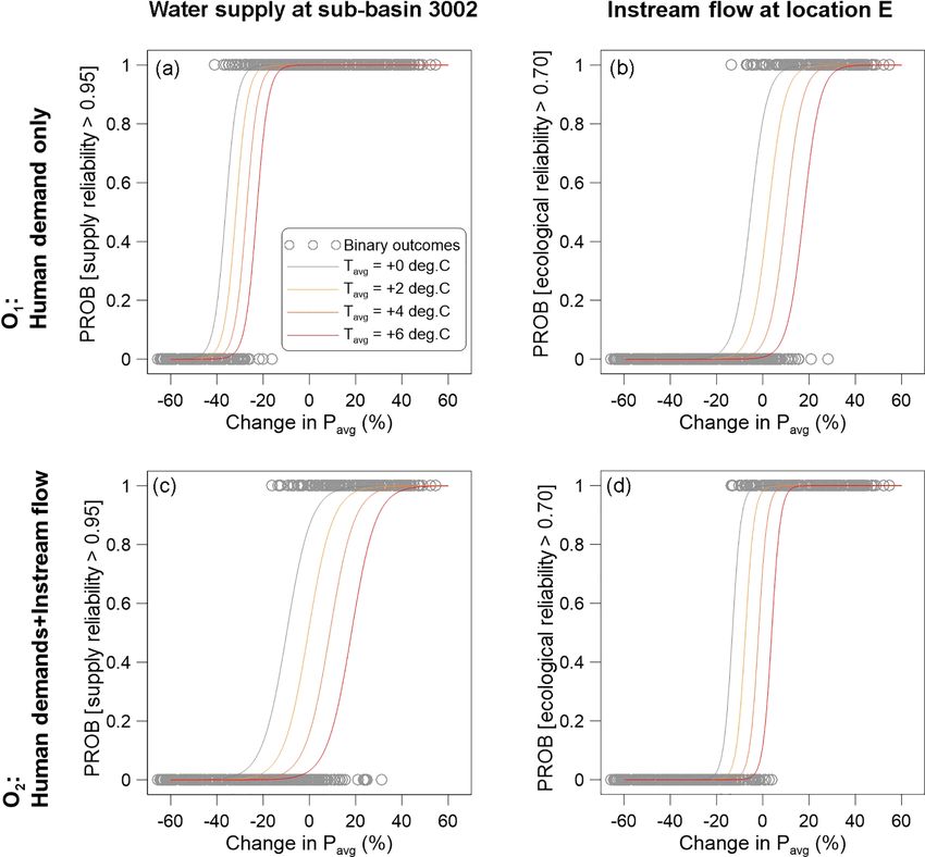
D. Kim et al.: Incorporating the logistic regression into a decision-centric impact assessment                                                    1149

Table 1. Annual agricultural and M & I demands per demand node, and the minimum instream flows from the sub-basins corresponding to
the seven locations.

                                        ID           Mean           Agricultural              M&I               Total         Instream flow
                                        no.         annual              demand              demand            storage           requirement
                                                     flow∗          (Mm3 yr−1 )          (Mm3 yr−1 )         capacity       (Mm3 month−1 )
                                                   3
                                                (Mm yr−1 )                                                    (Mm3 )
                                     3001               639.6                 50.9                 7.6           29.7
                                     3002                97.3                  4.0                 0.4            1.0
                                     3003               254.5                 13.1                 2.4            5.0
                                     3004               498.6                 50.5                15.8           10.1                   8.9 (A)
                                     3005               382.8                 42.3                 5.1           14.9                   6.6 (B)
                                     3006                82.6                  9.2                 3.3            6.8
                    Sub-basin        3007               384.0                 74.2                 6.1           22.0                   7.4 (C)
                    node             3008               473.6                 36.9                34.4            7.2
                                     3009               465.8                 31.5               208.5            7.0                   6.7 (D)
                                     3010                92.2                 19.3                16.4            0.2                  20.8 (E)
                                     3011              1145.0                356.6               296.2          100.9
                                     3012              1437.2                367.9                75.1           38.4                  45.9 (F)
                                     3013               506.1                193.2                26.4           47.4                   6.4 (G)
                                     3014               340.7                215.1                10.3           29.6
                    Outside          OD 1                                                          20.6
                    demand           OD 2                                                          42.1
                    node             OD 3                                                           5.1
                                     OD 4                                                           4.0
                             Total                     6800.0               1464.7               779.8          320.2
                  ∗ Natural runoff averaged over 20-year rainfall–runoff simulations with stochastic weather series containing zero climatic
                  perturbations (1Pavg = 0 %, 1Pcv = 0 %, and 1Tavg = 0 %) relative to 1996–2015. The letters A to G in the brackets are the
                  corresponding instream flow locations.

to 2030 given at 10-day intervals for the sub-basins and the                          ter allocation modeling, the demand data at 10-day intervals
two outside nodes directly linked to sub-basins from the                              were aggregated into monthly values.
team leading the national water plan at the Korea Institute
of Civil Engineering and Building Technology. Among the                               3.2.2      Bias-corrected GCM projections
three demand scenarios (high, medium, and low) given in
MOLIT (2016), we chose the high-demand scenario from a                                Daily precipitation and temperature projections of 25 GCMs
conservative perspective. More details about the demand pro-                          (Table A1) were collected from the archive of the Coupled
jections are available in MOLIT (2016). For simplicity, the                           Model Intercomparison Project Phase 5 (Taylor et al., 2012).
M & I demands at the two outside nodes connected with the                             Two representative concentration pathways (RCPs), RCP4.5
two dams were estimated by the water transfer records.                                and RCP8.5, were selected to assess the water supply ca-
   In addition, we collected the information of the minimum                           pacity of the river basin for the upcoming 20-year period
flow rates required for ecosystem sustainability, namely “in-                         of 2020–2039. RCP4.5 and RCP8.5 were used frequently as
stream flows” (Jowett, 1997), at seven locations within the                           scenarios of stabilized and increasing greenhouse gas con-
river basin. The instream flows are determined by the ex-                             centrations in climate change studies (e.g., Yan et al., 2015;
perts’ investigations into water quality and ecological con-                          Zhang et al., 2016; Moursi et al., 2017).
ditions in the vicinity of major rivers in South Korea and                               The 50 GCM projections (i.e., 25 GCMs × 2 RCPs) were
are officially announced by the Ministry of Environment and                           bias corrected by the de-trended quantile mapping (DQM;
the Ministry of Land, Infrastructure, and Transport (MOLIT,                           Bürger et al., 2013; Eum and Cannon, 2017) that can pre-
2016). Though the human water demands (i.e., agricultural                             serve raw climate change signals given by GCMs. The DQM
and M & I uses) are the first priority of the local and regional                      removes the long-term mean change in projected values first.
authorities (MOLIT, 2016), they are recommended for con-                              After applying the ordinary quantile mapping (QM; e.g.,
sidering the instream flows for environmental sustainability.                         Hwang and Graham, 2013) to the de-trended values, the re-
Table 1 summarizes the agricultural and M & I demands for                             moved trend is reintroduced to the bias-corrected projections.
the year of 2030 and the instream flow requirements. For wa-                          The de-trending procedure may prevent the exaggeration of
                                                                                      raw climate change signals, which is a typical drawback of

www.hydrol-earth-syst-sci.net/23/1145/2019/                                                             Hydrol. Earth Syst. Sci., 23, 1145–1162, 2019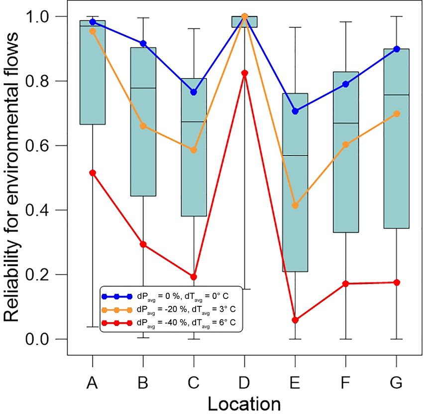
1150                         D. Kim et al.: Incorporating the logistic regression into a decision-centric impact assessment

the ordinary QM. More details about DQM and related bias-          series contain different internal variations. The 539 perturba-
correction methods are available in Bürger et al. (2013), Can-     tions were 11 changes in the average of daily precipitation,
non et al. (2015), and Eum and Cannon (2017). To correct           7 changes in the coefficient of variance (CV) of daily precip-
the 50 GCM projections toward the spatial averaged precip-         itation, and seven increases in the mean temperature over the
itation and temperatures over the Geum River basin, 1976–          20-year time horizons. The perturbations of mean precipita-
2005 and 2006–2099 were set as the reference and the pro-          tion were from −60 % to +40 % at 10 % increments relative
jection periods, respectively.                                     to the observations for 1973–2015, while the CV changes
                                                                   were from −40 % to +80 % at 20 % increments. The tem-
3.3     Stress tests for water allocation performances             perature perturbations were from +0 to +6 ◦ C at 1 ◦ C in-
                                                                   crements. The 539 (539 = 11 × 7 × 7) sets of climate-stress-
The stress tests were conducted for optimal water allocations      induced weather series were input to a rainfall–runoff model
in the node-and-link system. The 14 sub-basins are forced          to quantify natural water flows at the sub-basins. To develop
by atmospheric drivers (i.e., precipitation and temperature)       the logistic response surfaces, each weather series generated
to generate natural streamflow. The generated streamflows          by the WG was represented with the mean annual precipita-
are regulated to meet the water demands and instream flow          tion (Pavg ), the CV of daily precipitation (Pcv ), and the mean
requirements. The operations should be constrained by geo-         annual temperature (Tavg ) over the 20-year time horizon.
morphological and management conditions. We used a con-
ceptual runoff model and an optimization model for evaluat-        3.3.2   Simulating natural runoff at the sub-basin nodes
ing water supply and ecological performances with stochas-
tic weather series perturbed by hypothetical climate stresses.     A simple rainfall–runoff model, GR4J (Perrin et al., 2003),
                                                                   was used to simulate natural flows at the sub-basins nodes.
3.3.1    Generating climate-stress-induced weather series          GR4J has been frequently employed in many studies un-
                                                                   der diverse climates, such as parameter regionalization (e.g.,
The stochastic weather generator (WG) by Steinschneider            Oudin et al., 2010), predicting flow durations (e.g., Zhang
and Brown (2013) was employed to produce plausible daily           et al., 2015), and low flow estimations (e.g. Demirel et al.,
precipitation and temperature sequences with climatic pertur-      2015), among many others. GR4J uses four conceptual pa-
bations (i.e., generating climate stresses). Several bottom-up     rameters to describe functional behaviors of a watershed in
assessments successfully used this model to evaluate perfor-       response to lumped precipitation and potential evapotranspi-
mance of hydrologic systems under varying climate stresses         ration (PET) inputs. The parameters implicitly explain soil
(e.g., Whateley et al., 2014; Steinschneider et al., 2015b).       water storage, groundwater exchange, routing storage, and
The semi-parametric WG combines two stochastic mod-                excess runoff generations within a watershed. The parsimo-
els. The wavelet autoregressive model proposed by Kwon             nious structure of GR4J poses a relatively small equifinality
et al. (2007) first generates annual precipitation series spa-     problem in parameter calibration and regionalization (Oudin
tially averaged within a region of interest for a desired length   et al., 2008; Perrin et al., 2010). Perrin et al. (2003) provides
(20 years in this study). The wavelet components of the an-        the computation procedures in detail.
nual precipitation series are extended by the autoregressive          In the case study, a proximity-based regionalization was
model to embed the low-frequency structure inherent in ob-         applied for parameter identification because almost no natu-
servations. Then, daily weather series conditioned by the          ral streamflow observations are available at the outlets of the
random annual precipitation are simulated by the Marko-            sub-basins. The operational inflow records at the Yongdam
vian bootstrap resampler of Apipattanavis et al. (2007). In        Dam were the only applicable observations for parameter
this process, the daily observations are resampled by the          calibration at the sub-basin 3001. For the other sub-basins,
k-nearest-neighbor scheme and the precipitation occurrence         the parameter sets were transferred from neighboring water-
series generated by the standard Markovian process (e.g.,          sheds assessed in Kim et al. (2017). Kim et al. (2017) com-
Wilks, 1998). The weather data at multiple locations within        paratively assessed performance of the proximity-based pa-
the region of interest are sampled together for spatial coher-     rameter transfer in comparison to several alternative meth-
ence. For the final step, the mean and variance of stochastic      ods, concluding that spatial proximity captured functional
precipitation series are adjusted by the ordinary QM to im-        similarity well between 45 gauged watersheds in South Ko-
pose climatic perturbations stresses. The temperature series       rea. The mean Nash–Sutcliffe efficiency (NSE) was 0.53,
are simply perturbed by adding a temperature differential.         with a standard deviation of 0.41, when transferring the pa-
Further in-depth details about the stochastic WG are found         rameter sets of five neighboring catchments calibrated with
in Steinschneider and Brown (2013).                                observed hydrographs (Kim et al., 2017). Hence, for the
   Using the stochastic WG, we generated 539 sets of 20-           13 sub-basins from 3002 to 3014, natural flows were sim-
year-long precipitation and temperature time series perturbed      ulated with the transferred parameter sets from five nearby
by a combination of three climatic stresses for each set. Since    gauged watersheds, while flows at the sub-basin 3001 were
each weather series was newly generated, the 539 stochastic        generated by the parameters calibrated against the inflow

Hydrol. Earth Syst. Sci., 23, 1145–1162, 2019                                    www.hydrol-earth-syst-sci.net/23/1145/2019/
D. Kim et al.: Incorporating the logistic regression into a decision-centric impact assessment                              1151

data. The five runoff simulations were averaged for the sub-      ity (40 Mm3 month−1 ). The agricultural and M & I demands
basins in which the regionalization scheme was used. The pa-      were of equal priority in optimizations.
rameter set calibrated against the inflow records for the sub-       With 20-year-long natural flows per climatic perturbation,
basin 3001 yielded a NSE value of 0.62 for 2007–2015. The         we determined SAi , SMi , and Vi month by month using the
daily natural flows simulated by GR4J with the 539 climate-       global optimization tool “fmincon” in the Matlab software.
altered versions of the stochastic weather simulations were       Since Vi values determined for a month become water avail-
temporally aggregated at monthly values for water allocation      ability for the next month, optimizations for 240 months in-
modeling.                                                         teract sequentially. To consider the return flows, we followed
                                                                  the assumptions in the water plan for 2020 (MOLIT, 2016).
3.3.3   Water allocation modeling                                 Simply put, 65 % of the M & I water use at each node was
                                                                  assumed to return and become available water for following
The total water availability in the river basin during a cer-     nodes, while no return flows after agricultural uses were con-
tain month is water storage in the dams and reservoirs at the     sidered in the water plan due to high water use efficiency.
end of the previous month plus the natural flows at the sub-
basins in the current month. Some of the available water is       3.3.4    Evaluating water supply and ecological
again kept in the storage facilities for supplying water in up-            performances
coming months. Thus, operators’ decisions on water storage
in each month recursively affect supply performance in the        Using the optimized SAi , SMi , and Vi values, water sup-
river basin through a 20-year period. A monthly sequential        ply performances at the demand nodes were measured for
optimization model was used to determine amounts of the           the given 20-year-long stress-imposed weather series. For
water storage and consumption at each sub-basin. The oper-        each sub-basin node, we measured the water supply relia-
ators could minimize the water deficiency during a current        bility (ρs,i ) defined as the probability of satisfactory supply
month, while the water storage needs to be maximized for          against 99 % of the monthly demands:
water supplies in upcoming months. We assumed that the            ρs,i = prob [Si ≥ 0.99Di ] .                                (5)
two conflicting objectives are equally important for the op-
erators. Hence, the objective function for determining water      The amount of water passing through the seven locations
supplies and storage at the nodes for a particular month was      with the instream flow requirements can be also calculated
          P     P    P      P                                     using the decision variables and the natural flows. The en-
           Di − Si     Vi − Ci                                    vironmental reliability at an instream flow location j (ρe,j )
Minimize           −           ,                           (2)
                                                                  was evaluated by the following:
            P           P
              Di           Ci
Di = DAi + DMi ,                                           (3)
                                                                  ρe,j = prob Fj ≥ Fmin,j ,

                                                                                                                            (6)
Si = SAi + SMi ,                                           (4)
                                                                  where Fj and Fmin,j are the flow passing location j and the
where Di is the total demand, Si is the total supply, Vi is the   instream flows required for ecosystem sustainability at the
water storage, and Ci is the storage capacity (Ci ) at node i.    location, respectively.
SAi and SMi are agricultural, and M & I water supplied for           In total, water reliabilities at the 14 demand nodes (14 sub-
agricultural (DAi ) and M & I demands (DMi ) at node i. The       basins) and the seven locations requiring instream flows were
total water demand at each node (Di ) is the sum of agricul-      evaluated for each climatic perturbation. These 21 sets of
tural demand (DAi ) and M & I demand (DMi ). Likewise, the        performance indicators were used to develop the logistic re-
water supply at each node is divided into agricultural sup-       sponse functions for each sub-basin node and instream flow
ply (SAi ) and M & I supply (SMi ).                               location with corresponding climate stress. To develop the
   The monthly optimizations were subject to constraints.         logistic surfaces, we assumed that the stakeholder-driven
The water supply (Si ) to a demand node was limited by wa-        thresholds for ρs,i and ρe,j were 0.95 and 0.70, respectively.
ter availability, which is the sum of natural flow at the node    The 539 sets of Pavg , Pcv , and Tavg that represent the per-
in the current month, flows from other nodes via the stream       turbed weather series were categorized into zero and one
and the human-made links in the current month, and water          against the two thresholds for the logistic regressions.
storage at the node in the previous month. Water surplus at
the nodes was not allowed (i.e., Si ≤ Di ). The water remain-     4     Results
ing after supplies and storage at a sub-basin node should
be discharged from the node through the channel network.          4.1     Water supply performance at the sub-basins
The water storage at each node is constrained by its storage
capacity (Vi ≤ Ci ). The water transfers through the human-       The stress tests that forced the system models (i.e., GR4J
made links were only supplied for M & I demands of des-           and the optimization model) with the perturbed weather se-
tination nodes and were limited by the conveyance capac-          ries produced 539 sets of reliabilities for each sub-basin and

www.hydrol-earth-syst-sci.net/23/1145/2019/                                       Hydrol. Earth Syst. Sci., 23, 1145–1162, 2019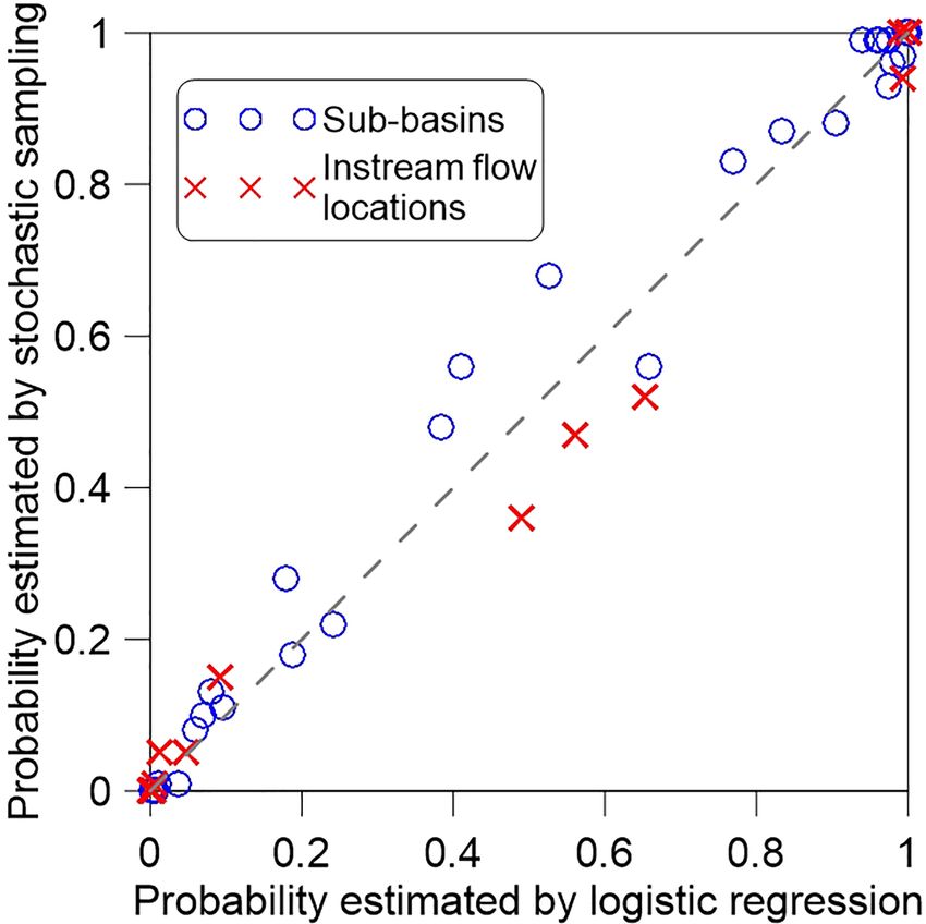
1152                           D. Kim et al.: Incorporating the logistic regression into a decision-centric impact assessment

Figure 2. Scatter plots between the water supply reliability at the sub-basin 3001 and changes in (a) Pavg , (b) Tavg , and (c) Pcv collected
from the stress tests driven by the 539 sets of stochastically generated stress-imposed weather series.

each location of instream flow. Figure 2 displays the scat-              ties of ρs > 0.95 (hereafter referred to as πs95 ) at the sub-
ter plots between water supply reliability (ρs ) at the sub-             basin 3001. πs95 declined with rising temperatures, since
basin 3001 and corresponding changes in Pavg , Pcv , and Tavg            water availability was reduced by evaporation losses. The
relative to 1996–2015. We preliminarily checked statistical              πs95 values indicated by the 50 GCMs ranged between 74 %
significance of the explanatory variables using the multiple             and 99 % for 2020–2039. It should be noted that the climatic
linear regressions. The changes in Pavg and Tavg were of                 bound for ρs = 0.95 (dashed lines in Fig. 3a and b) has the
very high significance to variation in the ρs values (p val-             risk of ρs < 0.95 as much as 40 %–60 % on the logistic sur-
ues < 10−16 ), whereas the change in Pcv was insignificant               faces. It seems that considerable risks of unsatisfactory per-
(p value = 0.744). This indicates that the water supply re-              formances still exist on the zone of satisfactory performance
liability is generally determined by variations of the mean              in Fig. 3a.
precipitation and temperature for a 20-year period. Though                  Likewise, we fitted the sigmoid functions to the binary
higher precipitation variability (Pcv ) could generate more di-          outcomes against the threshold of ρs > 0.95 for the other
rect runoff across the river basin, storage capacities of the            sub-basins. Figure 4 displays the climatic bounds at which
agricultural reservoirs and dams seem to nullify the impacts             πs95 = 95 % for each sub-basin. The sub-basin 3001 was of
of Pcv changes on the variation in water supply reliability.             the highest bound among the 14 sub-basins, indicating that
The preliminary regression analysis led us to a hypothesis               the uppermost sub-basin is the most vulnerable to changes
that changes in Pavg and Tavg could sufficiently capture the             in Pavg and Tavg . 15 GCMs were located below the climate
variation in water supply reliabilities across the river basin.          boundary of the sub-basin 3001. On the contrary, the bound-
   Figure 3a illustrates the multiple regression function be-            ary of the sub-basin 3012 was the lowest. For every GCM
tween the ρs values and changes in Pavg and Tavg (the coef-              projection, πs95 at the sub-basin 3012 was larger than 99 %.
ficient of determination is 0.93) on which the collection of             The sub-basins with limited connections to the upper sub-
50 GCM projections was overlaid. Most of the 50 GCMs                     basins tend to have higher climatic bounds of πs95 = 95 %.
expected that ρs at the sub-basin 3001 would be greater                  The lower sub-basins receiving streamflow generated by the
than 0.95 for 2020–2039. This type of response surfaces                  upper sub-basins are likely to withstand stronger climate
between expected performance and hypothetical climatic                   stresses, even though they have relatively large agricultural
stresses have been commonly used in the decision-centric as-             demands.
sessments (e.g., Brown et al., 2012; Whateley et al., 2014;
Turner et al., 2014). Figure 3c indicates that ρs at the sub-            4.2   Environmental reliability against the instream flow
basin 3001 could be less than 0.95 if Pavg decreases by ap-                    requirements
proximately 30 %. The ρs values varied significantly even
with zero decrease in Pavg , indicating that there might be              We compared the modeled flows at the seven locations of
the risk of unsatisfactory supply performance even with no               instream flow against the minimum requirements and evalu-
changes in Pavg .                                                        ated the environmental reliabilities (i.e., ρe ) at each location.
   The risk of ρs < 0.95 could be evaluated by the logis-                Figure 5 shows the box plots of ρe values at the seven lo-
tic surface shown in Fig. 3b. The sigmoid functions fitted               cations in response to the 539 climate perturbations. While
to the binary outcomes categorized against the threshold of              ρe values at all the locations decreased as climate became
ρs > 0.95 (Fig. 3d) could provide approximate probabili-                 drier, the location E was the most vulnerable. Even with
                                                                         no changes in Pavg and Tavg , the outflows from the sub-

Hydrol. Earth Syst. Sci., 23, 1145–1162, 2019                                           www.hydrol-earth-syst-sci.net/23/1145/2019/
D. Kim et al.: Incorporating the logistic regression into a decision-centric impact assessment 1153
Figure 3. (a) Response surface of ρs at the sub-basin 3011, and (b) logistic response surface of the probability of ρs > 0.95. (c) The scatter
plot between ρs and change in Pavg ; (d) the binary outcomes against the threshold of ρs > 0.95 and the sigmoid functions for the probability
of ρs > 0.95. The empty and filled circles overlaid on (a) and (b) are the 50 GCM projections for 2020–2039. The dashed lines in (a) and (b)
are the climatic bounds for the climatic threshold of ρs = 0.95. PROB stands for probability.
basin 3011 were often less than the minimum requirement,
implying that ecosystems near the location E might be cur-
rently undermined by the large agricultural and M & I de-
mands in the sub-basin 3011. If Pavg decreased by 20 % and
Tavg rose by 3 ◦ C, ρe at the location E would fall below 0.5.
In contrast, streamflow at the location D perfectly satisfied
the instream flow requirement under the same stress. Despite
the second-largest M & I demands in the sub-basin 3009, wa-
ter transfers from the two large dams could deliver sufficient
water supplies. 65 % of the water supplies for M & I demand
were supposed to return to the stream network and became
streamflow to meet the instream flow requirement at the lo-
cation D. Although both sub-basins 3009 and 3011 had lim-
ited geomorphological connectivity to the upper sub-basins,
their demand components and linkages to the two large dams
made the significant difference between their ρe values.
Figure 4. Climatic bounds for probability [ρs > 0.95] = 95 % for We developed the logistic response surfaces with binary
the 14 sub-basins on which the 50 GCM projections for 2020–2039 outcomes against the threshold of ρe > 0.70 at which the
were superimposed. instream flow requirement at the location E was satisfied
in the optimization model under no climate stresses (i.e.,
no changes in Pavg and Tavg relative to 1996–2015); Fig. 6
www.hydrol-earth-syst-sci.net/23/1145/2019/ Hydrol. Earth Syst. Sci., 23, 1145–1162, 20191154 D. Kim et al.: Incorporating the logistic regression into a decision-centric impact assessment
Figure 5. Reliability against the instream flow requirements at the Figure 6. As in Fig. 4, but for the probability of ρe > 0.70 at the
seven locations obtained from the 539 sequential optimizations with seven locations of instream flow.
stress-induced weather series. The blue, grey, and red lines connect
the reliabilities at the seven locations under the three representative
climatic stresses. stresses. Hence, it would be better to consider the instream
flow requirement in the objective function for the stress tests.
Through trial and error experiments with the 539 climate
displays the climatic bounds at which the probability of perturbations, we found that ρe at the location E could con-
ρe > 0.70 (hereafter referred to as πe70 ) is 95 % for all the siderably increase with a tiny w value. The sequential op-
locations requiring instream flow. As expected, the bound timizations with w = 0.01 allowed us to have a fairly im-
for the location E was the highest, and the climate zone proved ρe value at the location E. However, we found that
for πe70 > 95 % sensitively declines with rising Tavg . The the improved ecological reliability at the location E was from
bound for πs95 = 95 % at the sub-basin 3001 (black dashed substantial reduction in water supply reliability at the sub-
line) was below the bounds for the locations E. The human- basin 3002. Figure 7 illustrates the logistic models for water
demand-only operations would increase the risks of ecosys- supply at the sub-basin 3002 and the instream flow require-
tem degradation near the locations E if climate becomes ment at the location E under the two operation options ap-
drier. The environmental risks at the locations E seem to be plied to the case study. The first operation only considered
more sensitive to rising Tavg than the water supply risk at the the given agricultural and M & I demands (O1 ), whereas the
sub-basin 3001. Only 5 out of the 50 GCMs for 2020–2039 deficit against the instream flow requirement was considered
(10 %) indicate πe70 > 95 % at the location E. in the second option (O2 ). By changing the operation objec-
tive from O1 to O2 , the risk of ρe < 0.95 at the sub-basin sub-
4.3 Consideration of the instream flow into water stantially increased at the sub-basin 3002. The risk of unsatis-
management factory water supply was found even with increasing Pavg un-
der O2 . Indeed, the water supply performance became much
From the assessments with the logistic surfaces and the GCM
more sensitive to Tavg changes. Conversely, the risk of unsat-
projections, the environmental risk at the location E was
isfactory ecological reliability at the location E substantially
likely to become an issue for 2020–2039. As an adaptation
declined. This is because the optimization model could not
strategy, the instream flow could be considered in water man-
increase discharge from the sub-basin 3011 for the instream
agement to be balanced between water supply and environ-
flow requirement due to the high agricultural demands. In-
mental risks. We modeled this management option by includ-
stead, the model forced an increase in outflows from the
ing the instream flow requirement at the location E in the ob-
Yongdam Dam to meet the agricultural demands at the sub-
jective function of the water allocation model as
basins 3012 and 3014 and the instream flow at the location E.
It was inevitable to have deficient water supplies in the sub-
P P P P
Di − Si Vi − Ci Qmin,E − QE
Minimize P − P +w , (7) basin 3002 with relatively small demands, even under opti-
Di Ci Qmin,E
mized water allocations. In other words, minimizing the total
where Qmin,E and QE are the instream flow requirement and water deficiency of the entire basin may force the local water
flow at the location E, respectively. w is a weight represent- deficit in the sub-basin 3002.
ing relative importance of the instream flow in water manage-
ment. While the instream flow requirement at the location E
could be treated as a constraint for optimizations, this ap-
proach may lead to no optimal solutions under severe climate
Hydrol. Earth Syst. Sci., 23, 1145–1162, 2019 www.hydrol-earth-syst-sci.net/23/1145/2019/D. Kim et al.: Incorporating the logistic regression into a decision-centric impact assessment 1155
Figure 7. The logistic regression models for πs95 at the sub-basin 3002 (a, c) and πe70 at the location E (b, d) under the human-demand-only
operation (a, b), and the operation considering human demands and instream flow together (c, d).
4.4 Validating the logistic models and assessing the of (−37.1 %, +2.5 ◦ C), (−27.7 %, +1.3 ◦ C) and (−13.6 %,
management options with the EEDS framework +0.6 ◦ C) for both Pavg and Tavg . The change in Pcv was
fixed at a random value of +21 % because it was insignifi-
Since the sigmoid function is hypothetical, the logistic sur- cant to the regression models. Then, 100 sets of 20-year-long
faces need to be validated to ensure their predictive perfor- weather series were generated for each perturbation using
mance. As an interval validation (i.e., reusing the 539 sets the stochastic WG, and the system models were forced by
of performance samples for validation), the logistic models the generated weather series. By counting the cases satisfy-
were evaluated with the bootstrap prognoses (Harrell et al., ing ρs > 0.95 or ρe > 0.70 among the 100 simulations, the
1996). To measure the “optimism” of each logistic model, πs95 and πe70 estimates at the sub-basins and the instream
we used the Nagelkerke pseudo-R 2 (Nagelkerke, 1991; here- flow locations were obtained for each perturbation. Figure 8
after simply R 2 ) as the metric of predictive performance. compares the πs95 and πe70 estimates from the stress tests
The optimism of a regression model can be evaluated with against those estimated by the logistic models for the sub-
performance differences between the original model and the basins and the instream flow locations. The probability es-
models developed by bootstrap samples (with replacements). timates from the two methods seem to agree approximately.
Hence, it indicates a potential performance loss when apply- The median and the highest differences between the two es-
ing new samples to the original model. Together with the timates were 0.004 and 0.15, respectively.
regression results, Table 2 summarizes the optimism esti- The internal and external validations led us to believe that
mated from 2000 bootstrap models. Most of the logistic mod- the logistic surfaces could be acceptable for impact assess-
els showed 0.9 or higher R 2 values, and the highest opti- ments using the bias-corrected GCM projections. By over-
mism was only 0.80 %. The internal validation implies that lapping the logistic models, we could assess the two opera-
predictive performance of the logistic models seems accept- tion options applied in the case study for all the sub-basins
ably high and robust. As an external validation (i.e., valida- and the instream flow locations simultaneously (Fig. 9). For
tion with out-of-sample data), we conducted additional stress the assessment, we used the boundaries of πs95 = 95 % and
tests of the river system with three arbitrary perturbations
www.hydrol-earth-syst-sci.net/23/1145/2019/ Hydrol. Earth Syst. Sci., 23, 1145–1162, 20191156 D. Kim et al.: Incorporating the logistic regression into a decision-centric impact assessment
Table 2. The summary of logistic regressions and internal validations. The explanatory variables were statistically significant (p val-
ues < 10−3 ) for all the regression models.
O1 : human-demand-only operation O2 : considering the instream flow at E
Regression coefficients R 2,a Optimismb Regression coefficients R2 Optimism
Intersect 1Pavg 1Tavg Intersect 1Pavg 1Tavg
(%) (◦ C) (%) (◦ C)
3001 4.38 0.245 −0.630 0.91 0.0023 3.55 0.234 −0.529 0.90 0.0027
3002 14.5 0.401 −0.900 0.93 0.0035 1.86 0.189 −0.883 0.86 0.0029
3003 12.8 0.368 −0.776 0.94 0.0035 10.3 0.312 −0.605 0.92 0.0035
3004 14.1 0.388 −0.872 0.93 0.0037 13.1 0.363 −0.760 0.93 0.0034
3005 12.3 0.405 −0.724 0.94 0.0034 12.9 0.426 −0.806 0.94 0.0031
3006 16.8 0.430 −0.922 0.93 0.0033 13.6 0.354 −0.812 0.92 0.0032
3007 8.97 0.338 −0.866 0.94 0.0025 7.42 0.295 −0.812 0.93 0.0025
Sub-basin
3008 21.0 0.528 −1.03 0.94 0.0036 18.2 0.465 −0.954 0.94 0.0037
3009 10.3 0.302 −0.527 0.91 0.0031 10.3 0.302 −0.527 0.91 0.0037
3010 23.6 0.507 −0.654 0.94 0.0038 22.5 0.470 −0.761 0.93 0.0041
3011 11.2 0.383 −0.736 0.94 0.0030 11.9 0.410 −0.765 0.94 0.0028
3012 24.0 0.493 −0.825 0.93 0.0045 22.5 0.458 −0.790 0.92 0.0042
3013 11.4 0.292 −0.396 0.90 0.0036 11.0 0.284 −0.384 0.90 0.0038
3014 21.2 0.439 −0.690 0.92 0.0040 21.9 0.448 −0.729 0.92 0.0039
A 28.1 0.644 −1.69 0.96 0.0015 27.6 0.634 −1.67 0.96 0.0019
B 11.1 0.432 −1.11 0.95 0.0028 10.7 0.423 −1.00 0.95 0.0027
Instream C 6.43 0.370 −1.25 0.94 0.0033 6.51 0.399 −1.31 0.94 0.0028
flow D 25.9 0.445 −0.638 0.85 0.0068 21.1 0.402 −0.49 0.88 0.0052
locations E 1.47 0.282 −1.08 0.90 0.0033 7.02 0.533 −1.51 0.96 0.0016
F 5.44 0.332 −1.12 0.93 0.0032 6.52 0.385 −1.32 0.94 0.0023
G 14.1 0.591 −1.58 0.97 0.0017 13.0 0.547 −1.38 0.97 0.0022
a Nagelkerke pseudo-R 2 . b Mean performance loss in Nagelkerke pseudo-R 2 evaluated using 2000 bootstrap models.
πe70 = 95 %. With the logistic surfaces, the system robust-
ness to climate change could be measured in the same man-
ner proposed in the original EEDS framework (Poff et al.,
2016). Comparing Fig. 9b and e indicates that considering
the instream flow in the objective function significantly low-
ered the climatic bound of πe70 = 95 % at the location E,
thereby widening the climatic zone within which all the lo-
cations mutually satisfy πe70 > 95 %. However, in the trade-
off, the bound of πs95 = 95 % for the sub-basin 3002 moved
upward, narrowing the climatic zone mutually satisfying
πs95 > 95 % for all the demand nodes. Overall, the climatic
zone mutually satisfying πs95 > 95 % and πe70 > 95 % for
all the sub-basins and instream flow locations was expected
to decrease when the instream flow requirement at the loca-
tion E was considered. Based on the reduced mutual climate
Figure 8. 1 : 1 plots between the probability estimates from the zone, considering the environmental requirement in opera-
stochastic sampling and those from the logistic regressions for the tions would slightly decrease overall system robustness to
case study. The probabilities of satisfactory performance at the climate stresses.
14 sub-basins and the seven instream flow locations were estimated In summary, water supply reliabilities at the sub-
by the 100 Monte Carlo simulations for each climatic perturbation. basins 3001 and 3002 would be the most vulnerable to cli-
The number of points for comparison to the logistic models be- mate stresses. The highest environmental risks from climate
comes 63 (3 (perturbations) × 21 (locations) = 63.) change would be found at the locations E in terms of the
instream flow requirements. To reduce the environmental
Hydrol. Earth Syst. Sci., 23, 1145–1162, 2019 www.hydrol-earth-syst-sci.net/23/1145/2019/D. Kim et al.: Incorporating the logistic regression into a decision-centric impact assessment 1157
Figure 9. Climatic bounds for πs95 = 95 % (a, d) and πe70 = 95 % (b, e), and the bound mutually satisfying both criteria (c, f) under the
human-demand-only operations (a–c) in comparison to the operations considering the instream flows at the location E (d–f). The empty and
filled circles are the 50 GCM projections for 2020–2039.
risk at the location E, fairly increasing risks of ρs ≤ 0.95 at evaluation of the risk of system failures from a single cli-
the sub-basin 3002 should be accepted. Only 4 out of the mate projection. The probability estimates from the logistic
50 GCMs indicated πs95 > 0.95. surfaces can play a role in risk-based decision-making, par-
ticularly when an adaptive solution is targeted at a particular
climate prediction (e.g., resizing infrastructures for a refer-
5 Discussion and conclusions ence climate condition). The logistic surface developed for
the adaptive solution may directly provide the risk of sys-
5.1 Use of the logistic surfaces for the EEDS
tem failures under the climate prediction. Since it requires no
framework
more than a simple conversion of the sampled performance
metrics, the logistic regression allows a probabilistic evalu-
The response surfaces allowed users to estimate expected
ation of system performance in a very efficient manner. If a
performances of hydrologic systems in response to cli-
complex hydrologic system is assessed within the bottom-up
mate stressors, providing convenience in promptly evaluat-
framework, a typical approach such as an exhaustive Monte
ing many GCM projections (e.g., Turner et al., 2014; Brown
Carlo sampling may not be preferred for uncertainty analy-
et al., 2012; Prudhomme et al., 2010). Nevertheless, they
sis due to expensive computational costs. In such a case, the
could provide insufficient probabilistic information needed
logistic surfaces may become an alternative for simply as-
for decision-making processes. A possible approach for eval-
sessing the associated risks.
uating the risk of unsatisfactory performances was to count
The external validation of the logistic models (Fig. 8) im-
the GCM projections satisfying a predefined threshold (e.g.,
plies that the effect of interval climatic variability might be
Moursi et al., 2017; Brown et al., 2012). However, the GCM
measured in a collective manner, despite the varying climatic
counts are highly dependent on the size of the GCM collec-
perturbations of the weather series. Even though the pertur-
tions. Even in the case that all the GCMs in users’ hands fall
bations were different, the same probabilistic structure would
within the favorable climate zone on the response surfaces,
be inherent in all the generated weather series. This might
it does not guarantee that future system performance will be
allow the logistic models to collectively capture the effect
satisfactory at 100 % confidence.
of internal climate variability from the 539 weather series
The logistic response surface could supplement this weak-
having different climate alterations. Thus, uncertainty asso-
ness of the ordinary response surfaces. It enables the direct
www.hydrol-earth-syst-sci.net/23/1145/2019/ Hydrol. Earth Syst. Sci., 23, 1145–1162, 2019You can also read