Rotating shallow water flow under location uncertainty with a structure-preserving discretization - arXiv
←
→
Page content transcription
If your browser does not render page correctly, please read the page content below
Rotating shallow water flow under location uncertainty
                                                   with a structure-preserving discretization
                                                   Rüdiger Brecht† , Long Li§ , Werner Bauer‡ , Etienne Mémin§
                                                   † Department of Mathematics and Statistics, Memorial University of Newfoundland,
                                                   St. John’s (NL) A1C 5S7, Canada
                                                   §   Inria/IRMAR, Campus universitaire de Beaulieu, Rennes, France
                                                   ‡Imperial College London, Department of Mathematics, 180 Queen’s Gate, London SW7 2AZ,
                                                   United Kingdom.
arXiv:2102.03783v2 [physics.flu-dyn] 19 Oct 2021

                                                   Abstract
                                                   We introduce a physically relevant stochastic representation of the rotating shallow water equa-
                                                   tions. The derivation relies mainly on a stochastic transport principle and on a decomposition
                                                   of the fluid flow into a large-scale component and a noise term that models the unresolved flow
                                                   components. As for the classical (deterministic) system, this scheme, referred to as modelling
                                                   under location uncertainty (LU), conserves the global energy of any realization and provides the
                                                   possibility to generate an ensemble of physically relevant random simulations with a good trade-
                                                   off between the model error representation and the ensemble’s spread. To maintain numerically
                                                   the energy conservation feature, we combine an energy (in space) preserving discretization of
                                                   the underlying deterministic model with approximations of the stochastic terms that are based
                                                   on standard finite volume/difference operators. The LU derivation, built from the very same
                                                   conservation principles as the usual geophysical models, together with the numerical scheme
                                                   proposed can be directly used in existing dynamical cores of global numerical weather predic-
                                                   tion models. The capabilities of the proposed framework is demonstrated for an inviscid test
                                                   case on the f-plane and for a barotropically unstable jet on the sphere.

                                                   Plain summary
                                                   The motion of geophysical fluids on the globe needs to be modelled to get insights of tomorrow’s
                                                   weather. These forecasts must be precise enough while remaining computationally affordable.
                                                   Ideally they should enable to estimate likely scenarios through an ensemble of physically relevant
                                                   realizations, built from an accurate handling of the model errors that are inescapably introduced
                                                   due to physical or numerical approximations. To address these issues, we advocate the use of a
                                                   stochastic framework to represent the action of the many unresolved fast/small-scale processes
                                                   on the resolved flow component. The derivation of the stochastic system, based on the usual
                                                   conservation laws, is presented in detail and simulated with an adapted structure preserving
                                                   numerical model to maintain numerically the nice properties of the stochastic setting inherited
                                                   from a transport principle, namely: mass and energy conservation. The versatile nature of
                                                   the stochastic derivation as well as of the proposed numerical scheme makes this framework
                                                   suitable for existing dynamical cores of global numerical weather prediction models. Numerical
                                                   results illustrate the energy conservation of the numerical model and the accuracy of large-scale
                                                   stochastic simulations when compared to corresponding deterministic ones. The ability of the
                                                   random dynamical system to represent model errors is also shown.

                                                                                                   1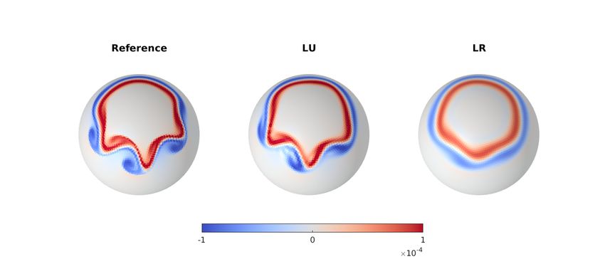
1    Introduction
Numerical simulations of the Earth’s atmosphere and ocean play an important role in developing
our understanding of weather forecasting. A major focus lies in determining the large-scale flow
correctly, which is strongly related to the parameterizations of sub-grid processes Frederiksen
et al. (2013). The non-linear and non-local nature of the dynamics of geophysical fluid flows
make the large-scale flow structures interact with the smaller components. Solving the Kol-
mogorov scales Pope (2000) of geophysical flows is today, and likely for a foreseeable future,
completely out of reach. This is due, in the first place, to the formidable computational ex-
pense that would be necessary, but also to the complexity of the many fine-scale physical or
bio-chemical processes involved. Truncating the fine scales and simply ignoring their actions
is highly detrimental to a reliable simulation of the large-scale components of the flow. Yet,
an accurate modelling of the fine-scale processes’ effects is an excruciatingly difficult task and
the idea of a stochastic modelling has strongly attracted the geophysical community since the
seminal works of Hasselmann (1976) and Leith (1975). For several years, this interest has been
strongly strengthened with the emergence of ensemble methods for probabilistic forecasting and
data assimilation issues Berner and Coauthors (2017); Franzke et al. (2015); Gottwald et al.
(2017); Majda et al. (2008); Palmer and Williams (2008); Slingo and Palmer (2011).
    The schemes proposed so far rely on very different methodological concepts. Multiplicative
random forcing and randomization of parameters based on early turbulence studies on energy
backscattering Leith (1990); Mason and Thomson (1992) have been proposed Buizza et al.
(1999); Porta Mana and Zanna (2014); Shutts (2005). The ad hoc nature of these schemes
makes a systematic stochastic derivation of any flow dynamical model or configuration difficult.
In addition, the absence of an explicit energy balance of the noise term leads to an uncontrolled
increase of variance that is potentially problematic. They consequently require a proper tuning
of the large-scale sub-grid model and of the noise amplitude to stabilize the system. The subgrid
model is, however, not related to the noise term and the amplitude of the perturbations to apply
is also difficult to specify on physical grounds. More importantly, even for low noise, an arbitrary
random perturbation defined outside of the physical principles on which the system has been
built upon may lead to strongly erroneous probability density functions of the system’s dynamics
Chapron et al. (2018). Other schemes based on an averaging and homogenization theory have
been proposed Franzke et al. (2006); Franzke and Majda (2006) in the wake of Majda et al. (1999)
and extended through the Mori-Zwanzig formalism (see the review Gottwald et al. (2017) and
references therein). Those techniques are well suited for the design of stochastic reduced order
systems.
    In this study, we propose to stick to a specific stochastic model, called modelling under
Location Uncertainty (LU) derived by Mémin (2014), which emerges from a decomposition of
the Lagrangian velocity into a smooth-in-time drift and a highly oscillating random term. Such
a slow/fast or smooth/oscillating decomposition is reminiscent to the Lagrangian decomposition
introduced in the seminal work of Andrews and McIntyre (1978), which is currently used for
surface or internal waves studies Kafiabad et al. (2021); Salmon (2013); Young and Jelloul
(1997); Xie and Vanneste (2015). A similar random decomposition is also at the center of the
variational stochastic framework of Holm (2015). Like our setting this latter approach applies
in a broader context and not only to wave solutions. Both frameworks rely on a stochastic
transport principle, with Holm (2015) dedicated to Hamiltonian dynamical systems and defined
from a circulation preserving constrained variational formulation, while Mémin (2014) is general
and built upon classical physical conservation laws.
    This stochastic transport principle has been used as a fundamental tool to derive stochas-
tic representations of large-scale geophysical dynamics Bauer et al. (2020a,b); Chapron et al.
(2018); Resseguier et al. (2017a,b,c) or to define large eddy simulation models of turbulent flows
Chandramouli et al. (2020); Kadri Harouna and Mémin (2017). The LU framework relies on a

                                                 2
stochastic representation of the Reynolds transport theorem Kadri Harouna and Mémin (2017);
Mémin (2014) which introduces naturally meaningful terms for turbulence studies.
It gathers a multiplicative random advection which is responsible for an energy backscattering,
a subgrid diffusion operator describing the mixing of the large-scale flow component by the small-
scale random component, and an effective advection which is attached to the small scales spatial
inhomogeneity. This latter term has been shown to be reminiscent of a generalized Stokes
drift component, hence designated as Itô-Stokes drift Bauer et al. (2020a). Backscattering and
diffusion are energetically in balance which leads hence to global energy conservation.
Recently, the LU formulation was shown to perform very well for oceanic quasi-geostrophic
flow models Resseguier et al. (2017b,c); Bauer et al. (2020a,b). It was found to be more accurate
in predicting the extreme events, in diagnosing the frontogenesis and filamentogenesis, in struc-
turing the large-scale flow and in reproducing long-terms statistics. Besides, for a LU version of
the Lorentz-63 model, derived from a Rayleigh-Bénard convection in the very same way as the
original model Berge et al. (1987); Lorenz (1963), it has been demonstrated that the LU setting
was more effective in exploring the range of the strange attractor compared to classical models
as well as to stochastic models built with ad hoc multiplicative forcings Chapron et al. (2018).
In this work, the performance of the LU representation is assessed for the numerical simu-
lation of the rotating shallow water (RSW) system, which can be considered as the first step
towards developing global random numerical weather prediction and climate models. In partic-
ular, this is the first time that the LU formulation is implemented for the dynamics evolving on
the sphere. The global energy conservation of the RSW-LU system for any realization, which
is analytically demonstrated here, is a strong asset of the approach and this invariant feature
should be numerically conserved as closely as possible. Global energy conservation is especially
important for long-term climatic simulations. However, classical purely damping parameteriza-
tions do not take into account energy and momentum fluxes from the unresolved to the resolved
scales. In climatic models, this is believed to be a source of important biases Gugole and Franzke
(2019).
Hence, we propose to combine the discrete variational integrator for RSW fluids as introduced
in Bauer and Gay-Balmaz (2019a) and Brecht et al. (2019) with the numerical LU setting in
order to maintain this conservation property as well as all the transport invariants. The benefit
of the proposed method that relies on a modular combination of a variational integrator with a
(potentially different) discretization of the LU formulation is that it should be directly applicable
to existing dynamical cores of numerical weather prediction models.
The derivation of the variational integrator is based on the variational discretization frame-
work introduced by Pavlov et al. (2011) for incompressible fluids, expanded by Gawlik et al.
(2011) to incompressible fluids with advected quantities. In various papers, this framework has
been further extended, for instance Desbrun et al. (2014) incorporated rotating and stratified
fluids of atmospheric and oceanic dynamics and Bauer and Gay-Balmaz (2019b) introduced
soundproof approximations of the Euler equations. Variational integrators are designed by first
discretizing the given Lagrangian, and then by deriving a discrete system of associated Euler-
Lagrange equations from the discretized Lagrangian (see Marsden and West (2001)).
The advantage of this approach is that the resulting discrete system inherits several important
properties of the underlying continuous system, notably a discrete version of Noether’s theorem
that guarantees the preservation of conserved quantities associated to the symmetries of the
discrete Lagrangian (see Hairer et al. (2006)). Variational integrators also exhibit superior
long-term stability properties, cf. e.g. Leimkuhler and Reich (2004). Therefore, they typically
outperform traditional integrators if one is interested in long-time integration or the statistical
properties of a given dynamical system. Our choice for an energy preserving rather than an
enstrophy conserving scheme is based on the following considerations. As shown in Bauer
et al. (2020b) for stochastic barotropic quasi-geostrophic models, using an energy conserving
scheme for long-term predictions yields better results than using an enstrophy conserving one.
3Besides, because of the direct cascade of enstrophy to high wave numbers, often stabilization
through enstrophy dissipation is introduced, even in initially enstrophy conserving schemes, cf.
Bonaventura and Ringler (2005); McRae and Cotter (2014); Ringler and Randall (2002).
Apart from taking into account the unresolved processes, it is paramount in probabilistic
ensemble forecasting to model the uncertainties along time Resseguier et al. (2020). In particular,
operational ensemble data assimilation methods rely classically on random perturbations of
the initial conditions (PIC) together with an artificially carefully inflated variance Anderson
and Anderson (1999) to increase the otherwise deficient ensemble forecasts’ spread Gottwald
and Harlim (2013); Franzke et al. (2015). Such inflation has the side effect of augmenting
also the representation error of the ensemble members. In the present work, we compare the
reliability of the ensemble spread of such a PIC model with our RSW-LU system, under the
same noise amplitude, and show that the LU strategy yields a good trade-off between model
error representation and ensemble spread.
The remainder of this paper is structured as follows. Section 2 describes the basic princi-
ples of the derivation of the rotating shallow water system in the LU formulation. Section 3
explains the numerical discretization of the stochastic dynamical system. Section 4 discusses
the numerical results for an inviscid test case with homogeneous noise and a viscous test case
with heterogeneous noise. In Section 5 we draw some conclusions and provide an outlook for
future work. In the Appendices we demonstrate the energy conservation of the RSW–LU sys-
tem, review some parameterizations of the noise and describe the discretization of the stochastic
terms.
2 Rotating shallow water equations under location uncertainty
In this section, we first review the LU representation introduced by Mémin (2014), then we derive
the rotating shallow water equations under LU, denoted as RSW–LU, following the classical
strategy Vallis (2017). In particular, we demonstrate one important characteristic of the RSW–
LU, namely that it preserves the total energy of the large-scale flow.
2.1 Location uncertainty principles
The LU formulation is based on a temporal-scale-separation assumption of the following stochas-
tic flow:
dX t = w(X t , t) dt + σ(X t , t) dB t , (2.1)
where X is the Lagrangian displacement defined within the bounded domain Ω ⊂ Rd (d =
2 or 3), w is the large-scale velocity that is both spatially and temporally correlated, and σdB t
is a highly oscillating unresolved component (also called noise) term that is only correlated in
space. The spatial structure of such noise is specified through a deterministic integral operator
σ : (L2 (Ω))d → (L2 (Ω))d , acting on square integrable vector-valued functions f ∈ (L2 (Ω))d ,
with a bounded kernel σ̆ such that
Z
σ[f ](x, t) = σ̆(x, y, t)f (y) dy, ∀f ∈ (L2 (Ω))d . (2.2)
Ω
The randomness of such a noise is driven by a functional Brownian motion B t Da Prato and
Zabczyk (2014). The fact that the kernel is bounded, implies that the resulting random flow
σdB t is a centered (of null ensemble mean) Gaussian process with the well-defined covariance
tensor :
h T i
Q(x, y, t, s) = E σ(x, t) dB t σ(y, s) dB s
4Z
= δ(t − s) dt σ̆(x, z, t)σ̆ T (y, z, s) dz, (2.3)
Ω
where E stands for the expectation, δ is the Kronecker symbol and •T denotes matrix or
vector transpose. The strength of the noise is measured by its variance, denoted here as a, and
which is given by the diagonal components of the covariance per unit of time:
a(x, t)dt = Q(x, x, t, t). (2.4)
We remark that this variance tensor has the same unit as a diffusion tensor (m2 · s−1 ) and
that the density of the turbulent kinetic energy (TKE) can be specified through it by 21 tr(a)/dt.
The previous representation (2.2) is a general way to define the noise, but other formulations
can be conveniently used in practice. In particular, the covariance operator per unit of time,
Q/dt, admits
P an orthogonal eigenfunction basis {Φn (•, t)}n∈N weighted by the eigenvalues Λn ≥ 0
such that n∈N Λn < ∞. Therefore, one may equivalently define the noise and its variance, based
on the following spectral decomposition:
X X
σ(x, t) dB t = Φn (x, t) dβtn , a(x, t) = Φn (x, t)ΦTn (x, t), (2.5)
n∈N n∈N
where β n denotes n independent and identically distributed (i.i.d.) one-dimensional stan-
dard Brownian motions. The specification of those basis functions from data driven empirical
covariance matrices enables one to construct specific noises, informed either by numerical or ob-
servational data. This strategy will allow us to devise various forms of the noise in the following.
Remark 1 Decomposition 2.1 is a temporal decomposition and not a spatial decomposition
as classically formulated through spatial filters and/or decimation operators in large-eddies sim-
ulation (LES) techniques. However, in the case of turbulent flows, time and spatial scales are
related. As a matter of fact, in the inertial range, the turn-over time ratio for two different
scales L and ` reads τL /τ` ∝ (L/`)2/3 and provides a direct relation between time-scale coarsen-
ing and spatial-scale dilation. Unless specifically needed, in the following, we will thus refer to
large/small or unresolved scales without differentiating between time or space scales. Note also
that temporal filtering has already been used for the definition of oceanic models Hecht et al.
(2008) or large-eddies simulation approaches Meneveau and Katz (2000).
Remark 2 Decomposition 2.1 is written in terms of an Itô stochastic integral. This decom-
position could have been written in the form of a Stratonovich integral as well. The calculus
associated to this latter integral has the advantage of following the classical chain rule. However,
the Stratonovich noise no longer has zero expectation. This leads thus to a problematic decom-
position with velocity fluctuations of non null ensemble mean. For smooth enough integrands,
it is possible to safely move from one form to the other. For interested readers, more insights
on the difference of the two settings and their implications in stochastic oceanic modelling are
provided in Bauer et al. (2020a).
Remark 3 The approach could be extended to express flows on arbitrary Riemannian man-
ifolds. In that case it is easier to work directly with the Stratonovich formulation since it is
invariant under the change of coordinates. As we consider here only flows that assume the
shallow approximation, the considered representation of the equations in R2 and R3 is a very
accurate approximation.
The core of the LU model representation is based on a stochastic Reynolds transport theorem
(SRTT), introduced by Mémin (2014), which describes the rate of change of a random scalar q
5transported by the stochastic flow (2.1) within a flow volume V. In particular, for incompressible
unresolved flows, ∇·σ = 0, the SRTT can be written as
Z Z
dt q(x, t) dx = Dt q + q ∇· (w − ws ) dx, (2.6a)
V(t) V(t)
1
Dt q = dt q + (w − ws ) ·∇ q dt + σdB t ·∇ q − ∇· (a∇q) dt, (2.6b)
2
where dt q(x, t) = q(x, t + dt) − q(x, t) stands for the forward time-increment of q at a fixed
point x, Dt is introduced as the stochastic transport operator in Resseguier et al. (2017a) and
ws = 12 ∇· a is referred to as the Itô-Stokes drift (ISD) in Bauer et al. (2020a). The transport
operator plays the role of the material derivative in the stochastic setting. The ISD is defined
by the variance tensor divergence and embodies the effect of statistical inhomogeneity of the
unresolved flow on the large-scale component. As shown in Bauer et al. (2020a), it can be
considered as a generalization of the Stokes drift associated to waves propagation with the
emergence of a similar vortex force and Coriolis correction. In the definition of the stochastic
transport operator in (2.6b), the last two terms describe, respectively, an energy backscattering
from the unresolved scales to the large scales and an inhomogeneous diffusion of the large
scales driven by the variance of the unresolved flow components. The diffusion term generalizes
the Boussinesq eddy viscosity assumption (here with a matrix eddy viscosity). This term is,
nevertheless, directly related to the noise form and not anymore defined by loose analogy with
the molecular dissipation mechanism. The backscattering term corresponds to an energy source
that is exactly compensated by the diffusion term Resseguier et al. (2017a).
In particular, for an isochoric flow with ∇·(w − ws ) = 0, one may immediately deduce from
(2.6a) the following transport equation of an extensive scalar:
Dt q = 0, (2.7)
where the energy of such random scalar q is globally conserved, as shown in Resseguier et al.
(2017a):
Z 1 1Z 1
Z
dt q 2 dx = q ∇· (a∇q) dx + (∇q)T a∇q dx dt = 0. (2.8)
Ω 2 2 2
| Ω {z } | Ω {z }
Energy loss by diffusion Energy intake by noise
Indeed, this can be interpreted as a process where the energy brought by the noise is exactly
counterbalanced by that dissipated from the diffusion term.
2.2 Derivation of RSW–LU
This section describes in detail the derivation of the RSW–LU system. This model enriches the
formulation described in Mémin (2014). Here it is fully stochastic and includes rotation to suit
simulations of geophysical flows on a rotating frame.
The above SRTT (2.6a) and Newton’s second principle allow us to derive the following (three-
dimensional) stochastic equations of motions in a rotating frame Bauer et al. (2020a):
Horizontal momentum equation :
1
Dt u + f × u dt + σ H dB t = − ∇H p dt + dpσt + ν∇2 u dt + σ H dB t ,
(2.9a)
ρ
Vertical momentum equation :
61
Dt w = − ∂z p dt + dpσt − g dt + ν∇2 w dt + σz dBt ,
(2.9b)
ρ
Mass equation :
Dt ρ = 0, (2.9c)
Continuity equations :
∇H · u − us + ∂z (w − ws ) = 0, ∇H · σ H dB t + ∂z σz dBt = 0, (2.9d)
where u = (u, v)T (resp. σ H dB t ) and w (resp. σz dBt ) are the horizontal and vertical
components of the three-dimensional large-scale flow w (resp. the unresolved random flow
σdB t ); f = (2Ω̃ sin Θ)k is the Coriolis parameter varying in latitude Θ, with the Earth’s angular
rotation rate Ω̃ and the vertical unit vector k = [0, 0, 1]T ; ρ is the fluid density; ∇H = [∂x , ∂y ]T
denotes the horizontal gradient; p and ṗσt = dpσt /dt (informal definition) are the time-smooth
and time-uncorrelated components of the pressure field, respectively; g is the Earth’s gravity
value and ν is the kinematic viscosity. In the following, the molecular friction term is assumed to
be negligible and dropped from the equations. Note that in our setting the continuity equations
(2.9d) ensure volume conservation Resseguier et al. (2017a) and mass conservation (2.9c).
In order to model the large-scale circulations in the atmosphere and ocean, the hydrostatic
balance approximation is widely adopted Vallis (2017). We now specify the scaling for this
balance in the LU framework. We first adimensionalize the basic variables as
(x, y) = L (x0 , y 0 ), u = U u0 , t = T t0 , T = L/U, z = αLz 0 , α = H/L, (2.10)
where the capital letters are used for the characteristic scales of variables and •0 denotes
adimensional variables. To scale properly the vertical velocity, we propose to adopt a sufficient
incompressible condition Resseguier et al. (2017a,b) for the resolved component in Equation
(2.9d), that is
∇H · u + ∂z w = 0, ∇H · us + ∂z ws = 0. (2.11)
Note that the latter divergence-free condition on the ISD is usually considered for the classical
Stokes drift McWilliams et al. (2004) although being controversial Mellor (2016). The three-
dimensional bolus velocity introduced in the eddy-induced-advection parametrization Gent and
McWilliams (1990); Gent et al. (1995); Griffies (1998) is also assumed to be incompressible in
order to preserve the tracer’s moments. In our case, the justification of this constraint is further
strengthen by global energy conservation and a desirable bridge between the classical (global
energy conserving) rotating shallow water system and its stochastic representation. Under the
condition (2.11), a classical scaling of the vertical (resolved) velocity holds:
w = α U w0 . (2.12)
Apart from these classical scaling numbers, the horizontal component aH of the variance/diffusion
tensor a, which characterizes the strength of the unresolved component, is scaled as
0 aH aHz Tσ EKE
aH = UL aH , a= , = , (2.13)
aHz az T MKE
where the specific factor Resseguier et al. (2017b) is defined as the ratio between the eddy
kinetic energy (EKE) and the mean kinetic energy (MKE), multiplied by the ratio between the
7unresolved scale correlation time Tσ and the large-scale advection time. From the definitions
(2.3) and (2.4), the scaling of the horizontal small-scale flow reduces to
√
σ H dB t = L (σ H dB t )0 . (2.14)
In addition, we consider the following scaling between the vertical and horizontal components
of the unresolved flow:
σz dBt √
∼ α δ, i.e. σz dBt = δ H (σz dBt )0 , (2.15)
kσ H dB t k
where δ is a small factor Resseguier et al. (2017b). Again, from the definitions (2.3) and
(2.4), the other components of the variance/diffusion tensor scale then as:
az
aHz = δ UH a0Hz , az = δ 2 α UH a0z , i.e. ∼ α2 δ 2 . (2.16)
kaH k
This relation provides a ratio between the vertical and horizontal eddy diffusivities. It is in
practice quite small at large scale Lévy et al. (2010, 2012).
Now, with f = 0 and a constant density ρ0 , the horizontal momentum equation (2.9a) implies
the following scalings of the rescaled pressures:
√
p̃ = p/ρ0 = U 2 p̃0 , dp̃σt = dpσt /ρ0 = UL (dp̃σt )0 . (2.17)
Finally, substituting all the above scalings into Equation (2.9b), the adimensional vertical
momentum is given by
√
2
dt w0 + (u0 · ∇0H w0 + w0 ∂z0 w0 ) dt0 + (σ H dB t )0 · ∇0H w0 + δ (σz dBt )0 ∂z0 w0
α
0
− (∇H · a0H + δ ∂z0 a0Hz ) · ∇0H w0 + δ (∇0H · a0Hz + δ ∂z0 a0z )∂z0 w0
2
+ ∇H · (aH ∇H w + δ aHz ∂z w ) + δ ∂z (aHz ∇H w + δ az ∂z w ) dt0
0 0 0 0 0 0 0 0 0 0 0 0 0 0
√ 1
= −∂z0 p̃0 dt0 + (dp̃σt )0 − 2 dt0 ,
(2.18)
Fr
√
where Fr = U/ gH is the Froude number. Let us now make the following assumptions:
α2
1, Fr2 = O(1), = O(1), δ
1. (2.19)
The acceleration term on the left-hand side (LHS) of Equation (2.9b) has now a lower order
of magnitude than the RHS terms. Restoring the dimensions, the hydrostatic balance under
moderate horizontal uncertainty and weak vertical uncertainty hence boils down to
∂z p dt + dpσt = −ρg dt, i.e. ∂z p = −ρg, ∂z dpσt = 0.
(2.20a)
We remark that the unique decomposition principle of a semimartingale process Kunita (1997)
is used here to separate the bounded variation component (in terms of dt) and the martingale
part (in terms of dB t or dpσt ). Integrating vertically these hydrostatic balances (2.20a) from 0
8Figure 1. Illustration of a single-layered shallow water system (inspired by Vallis (2017)). h is the thickness of a
water column, η is the height of the free surface and ηb is the height of the bottom topography. As a result, we
have h = η − ηb .
to z (see Figure 1), we have
p(x, y, z, t) = p0 (x, y, t) − ρ0 gz, dpσt (x, y, z, t) = dpσt (x, y, 0, t), (2.20b)
where p0 denotes the pressure at the bottom of the basin (z = 0). Following Vallis (2017), we
assume that the weight of the overlying fluid is negligible, i.e. p(x, y, η, t) ≈ 0 with η the height
of the free surface, leading to p0 = ρ0 gη. This allows us to rewrite Equation (2.20b) such that
for any z ∈ [0, η] we have
p(x, y, z, t) = ρ0 g η(x, y, t) − z . (2.20c)
Subsequently, the pressure gradient force in the horizontal momentum equation (2.9a) reads
1 1
∇H p dt + dpσt = −g∇H η − ∇H dpσt ,
− (2.20d)
ρ0 ρ0
which does not depend on z according to Equations (2.20b) and (2.20c). Therefore, the
acceleration terms on the LHS of Equation (2.9a) cannot depend on z, and the shallow water
momentum equation under weak vertical uncertainty (δ
1) can be written finally as
1
∇H dpσt ,
DH
t u + f × u dt + σ H dB t = −g∇H η dt − (2.21a)
ρ0
1
DH
t u = dt u + (u − us ) dt + σ H dB t · ∇H u − ∇H · aH ∇H u dt, (2.21b)
2
where us = 12 ∇H · aH is the two-dimensional ISD and DH t denotes the horizontal stochastic
transport operator whose expression is recalled in (2.21b) for the u component. The relation
between the unresolved flow component and the random pressure can be further specified by
considering a scaling of the martingale part of the momentum equation:
√
√ 0 √ 0 0 0 √
dt ũ + (σ H dB t ) · ∇H u + f 0 × (σ H dB t )0 = ∇0H (dpσt )0 , (2.22)
Ro
where Ro = U/(f0 L) denotes the Rossby number with f = f0 f 0 , and ũ = u − E(u) stands
√
for the martingale part of the horizontal velocity. We note that the scaling dt ũ = U dt ũ0
9is obtained from the variance of the martingale part of the vertical acceleration term (2.18)
considering the hydrostatic balance (2.20a) and the continuity equation (2.11). Therefore, for
small Rossby number (Ro ≤ 1), the random Coriolis term counter-balances the random gradient
pressure force:
1
f × σ H dB t ≈ − ∇H dpσt . (2.23)
ρ0
Besides, under weak vertical uncertainty, the dimensional continuity equations (2.11) and
(2.9d) reduce to
∇H · σ H dB t = ∇H · us = 0. (2.24)
As a result, the vertical integration (from bottom topography ηb to free surface η) of the
continuity equations (2.9d) become
(w − ws )|z=η − (w − ws )|z=ηb = −h∇H · u, σdBt |z=η − σdBt |z=ηb = 0, (2.25a)
where h = η − ηb denotes the thickness of the water column (with a still bottom). On the
other hand, a small vertical (Eulerian) displacement at the top and bottom of the fluid leads to
a variation of the position of a particular fluid element Vallis (2017):
(w − ws ) dt + σdBt z=η
= DH
t η, (w − ws ) dt + σdBt z=ηb
= DH
t ηb . (2.25b)
Combining Equations (2.25), we deduce the following stochastic mass equation:
DH
t h + h∇H · u dt = 0. (2.26)
Gathering all the elements derived so-far, we finally obtain the following RSW-LU system
(Conservation of momentum)
Dt u + f × u dt = −g∇η dt, (2.27a)
(Conservation of mass)
Dt h + h ∇· u dt = 0, (2.27b)
(Random balance)
1
f × σdB t = − ∇dpσt , (2.27c)
ρ
(Incompressible constraints)
∇· σdB t = 0, ∇·us = 0, (2.27d)
where the symbol H for all horizontal variables are dropped for readability reasons. In A it
is shown that this stochastic system conserves the global energy:
ρ
Z
h|u|2 + gh2 dx = 0.
dt (2.28)
Ω 2
It shares thus exactly the same energy conservation property as the deterministic one and
beyond their formal resemblance this provides a strong physical link between the two systems.
Moreover, it can be noticed that under a sufficiently weak (horizontal) uncertainty (σ ≈ 0), the
system (2.27) reduces to the classical RSW system, in which the stochastic transport operator
weighted by the unit of time, Dt /dt, reduces to the material derivative.
103 Structure-preserving discretization of RSW–LU
In order to perform numerical simulations of the RSW–LU (2.27) the noise term σdB t has to
be a priori parametrized. Its shape is conveniently expressed through a spectral representation
and a set of basis functions (2.5). In this work homogeneous as well as heterogeneous spatial
structures have been used and the way they are defined is reviewed in B. The incompressible
homogenous noise (see Appendix B.1) is defined through a convolution kernel and is associated
with Fourier modes orthogonal functions. It is easy to implement through fast Fourier transform
(FFT). As shown in Section 4.1, this noise was in particular used to assess the numerical energy
behavior of the discrete scheme. However, homogeneous noises, although carefully scaled from
a known energy spectrum established at high resolution, fail to represent inhomogeneity effect
encoded by spatially varying variance (the variance is constant and diagonal for homogeneous
incompressible noise). This is detrimental to represent large scale effects shaped by the small-
scale components in geophysical fluid dynamics. As a matter of fact as shown in Bauer et al.
(2020a), heterogeneous noise shapes the large-scale flow in a way akin to the action of vortex
force associated with the classical Stokes drift.
In this work, two different parameterizations of heterogeneous noise have been used and
are described in Appendix B.2. The former consists in calibrating empirical orthogonal basis
functions (EOF) before the simulation (off-line) from available high-resolution simulation data
while the latter consists in specifying the basis functions from the on-going (low resolution)
simulation (i.e. on-line). The second basis functions do not depend on data and are time
evolving whereas the first ones are data driven and stationary. A procedure based on dynamic
mode decomposition Schmid (2010) to define the noise through evolving basis functions could
have been as well used, as proposed by Gugole and Franzke (2019). Such a time evolving
basis, learned from a high resolution simulation, are shown to perform better that stationary
EOF based models. We will have the same type of conclusions for the non-stationnary noise
experimented here. In Section 4.2, both heterogeneous noises are adopted for identifying the
barotropic instability of a mid-latitude jet.
In the following, we focus on an energy conserving (in space) approximation of the random
dynamical system (RSW–LU). In this context, the spatial discretization allows us to mimic the
balance between the global energy brought by the noise and the LU-diffusion (see Eqn. 2.8) at
each time step, hence no additional numerical dissipation or energy increase is introduced into
the system. Considering the definition of the stochastic transport operator Dt in (2.6b), the
RSW–LU system in Eqn. (2.27a)–(2.27b) can be explicitly written as
1
dt u = − u ·∇ u − f × u − g∇η dt + ∇· ∇·(au) dt − σdB t ·∇ u , (3.1a)
2
1
dt h = − ∇· (uh) dt + ∇· ∇·(ah) dt − σdB t ·∇ h . (3.1b)
2
We suggest to develop an approximation of the stochastic RSW–LU model (3.1a)–(3.1b)
by first discretizing the deterministic model underlying this system with a structure-preserving
discretization method (that preserves energy in space) and, then, to approximate (with a po-
tentially different discretization method) the stochastic terms. Here, we use for the former a
variational discretization approach on a triangular C–grid while for the latter we apply a stan-
dard finite difference method. Note that for the methodology introduced in this manuscript,
other spatially energy conserving discretizations rather than the suggested variational integra-
tor could be used too. The deterministic dynamical core of our stochastic system results from
simply setting σ ≈ 0 in the equations (3.1a)–(3.1b). To obtain the full discretized (in space
and time) scheme for this stochastic system, we wrap the discrete stochastic terms around the
deterministic core and combine this with an Euler–Marayama time scheme.
11Introducing discretizations of the stochastic terms that do not necessarily share the same
operators as the deterministic scheme has various advantages, as discussed in more detail in
Section 3.2.1. For instance, such a well defined interface between these two model components
minimizes the necessity to adapt the discretization schemes to each other which, in turn, would
permit us to apply our method immediately to existing dynamical cores of global numerical
weather prediction (NWP) models.
3.1 Discretization of deterministic RSW equations
As mentioned above, the deterministic model (or deterministic dynamical core) of the above
stochastic system results from setting σ ≈ 0, which leads via (2.4) to a ≈ 0. Hence, Equations
(3.1a)–(3.1b) reduce to the deterministic RSW equations
1
dt u = − (∇ × u + f ) × u − ∇( u2 ) − g∇η dt, dt h = − ∇· (uh) dt, (3.2)
2
where we used the vector calculus identity u ·∇ u = (∇ × u) × u + 12 u2 . Note that in the
deterministic case dt /dt agrees (in the limit dt → 0) with the partial derivative ∂/∂t.
3.1.1 Variational discretizations
In the following we present an energy conserving (in space) approximation of these equations
using a variational discretization approach. While details about the derivation can be found in
Bauer and Gay-Balmaz (2019a); Brecht et al. (2019), here we only give the final, fully discrete
scheme.
To do so, we start with introducing the mesh and some notation. The variational discretiza-
tion of (3.2) results in a scheme that corresponds to a C-grid staggering of the variables on a
quasi uniform triangular grid with hexagonal/pentagonal dual mesh. Let N denote the number
of triangles used to discretize the domain. As shown in Fig. 2, we use the following notation:
T denotes the primal triangle, ζ the dual hexagon/pentagon, eij = Ti ∩ Tj the primal edge and
ẽij = ζ+ ∩ ζ− the associated dual edge. Furthermore, we have nij and tij as the normalized
normal and tangential vector relative to edge eij at its midpoint. Moreover, Di is the discrete
water depth at the circumcentre of Ti , ηb i the discrete bottom topography at the circumcentre
of Ti , and Vij = (u · n)ij the normal velocity at the triangle edge midpoints in the direction
from triangle Ti to Tj . We denote Dij = 12 (Di + Dj ) as the water depth averaged to the edge
midpoints.
The variational discretization method does not require to define explicitly approximations of
the differential operators because they directly result from the discrete variational principle. It
turns out that on the given mesh, these operators agree with the following definitions of standard
finite difference and finite volume operators:
FT − FTi 4 1 X
4 (Div V )i = |eik |Vik ,
(Gradn F )ij = j , |Ti |
|ẽij | k∈{j,i− ,i+ }
(3.3)
4 Fζ − Fζ+ 4 1 X
(Gradt F )ij = − , (Curl V )ζ = |ẽnm |Vnm ,
|eij | |ζ|
ẽnm ∈∂ζ
for the normal velocity Vij and a scalar function F either sampled as FTi at the circumcentre
of the triangle Ti or sampled as Fζ± at the centre of the dual cell ζ± . The operators Gradn and
Gradt correspond to the gradient in the normal and tangential direction, respectively, and Div
to the divergence of a vector field:
12Tj−
ζ− ẽjj−
Ti− ẽii− eij
Tj ẽjj+
Ti
Tj+
ẽii+ ζ+
Ti+
Figure 2. Notation and indexing conventions for the 2D simplicial mesh.
(∇F )ij ≈ (Gradn F )nij + (Gradt F )tij , (3.4)
(∇ · u)i ≈ (Div V )i , (3.5)
(∇ × u)ζ ≈ (Curl V )ζ . (3.6)
The last equation defines the discrete vorticity and for later use, we also discretize the po-
tential vorticity as
∇×u+f (Curl V )ζ + fζ X |ζ ∩ Ti |
≈ , Dζ = Di . (3.7)
h Dζ |ζ|
ẽij ∈∂ζ
3.1.2 Semi-discrete RSW scheme
With the above notation, the deterministic semi-discrete RSW equations read:
dt Vij = LVij (V, D) ∆t, for all edges eij , (3.8a)
dt Di = LD
i (V, D) ∆t, for all cells Ti , (3.8b)
where LVij and LD
i denote the deterministic spatial operators, and ∆t stands for the discrete
time step. The RHS of the momentum equation (3.8a) is given by
4
LVij (V, D) = −Adv(V, D)ij − K(V )ij − G(D)ij , (3.9)
where Adv denotes the discretization of the advection term (∇ × u + f ) × u of (3.2), K the
approximation of the gradient of the kinetic energy ∇( 12 u2 ) and G of the gradient of the height
13field g∇η. Explicitly, the advection term is given by
4
Adv(V, D)ij =
1 |ζ ∩ T | |ζ− ∩ Tj |
− i
− (Curl V )ζ− + fζ− Dji− |eii− |Vii− + Dij− |ejj− |Vjj−
Dij |ẽij | 2|Ti | 2|Tj | (3.10)
1 |ζ+ ∩ Ti | |ζ+ ∩ Tj |
+ (Curl V )ζ+ + fζ+ Dji+ |eii+ |Vii+ + Dij+ |ejj+ |Vjj+ ,
Dij |ẽij | 2|Ti | 2|Tj |
where fζ± is the Coriolis term evaluated at the centre of ζ± . Moreover, the two gradient
terms read:
4 1
X |ẽik | |eik |(Vik )2
K(V )ij = (Gradn F )ij , FTi = , (3.11)
2 2|Tk |
k∈{j,i− ,i+ }
4
G(D)ij = g(Gradn (D + ηb ))ij . (3.12)
The RHS of the continuity equation (3.8b) is given by
4
LD
i (V, D) = − Div (DV ) i , (3.13)
which approximates the divergence term − ∇· (uh).
3.1.3 Time scheme
For the time integrator we use a Crank-Nicolson-type scheme where we solve the system of fully
discretized non-linear momentum and continuity equations by a fixed-point iterative method.
The corresponding algorithm coincides for σ = 0 with the one given in Section 3.3.
3.2 Spatial discretization of RSW–LU
The fully stochastic system has additional terms on the RHS of Equations (3.1a) and (3.1b).
With these terms the discrete equations read:
dt Vij = LVij (V, D) ∆t + ∆Gij
V
, (3.14a)
dt Di = LD D
i (V, D) ∆t + ∆Gi , (3.14b)
where the stochastic LU-terms are given by
∆t
V 4
∆Gij = ∇ · ∇· (au) ij − (σdB t ·∇ u)ij · nij , (3.14c)
2
4 ∆t
∆GiD = ∇ · ∇· (aD) i − (σdB t ·∇ D)i . (3.14d)
2
Note that the two terms within the large bracket in (3.14c) comprise two Cartesian compo-
nents of a vector which is then projected onto the triangle edge’s normal direction via nij . The
two terms in (3.14d) are scalar valued at the cell circumcenters i.
The parametrization of the noise described in B is formulated in Cartesian coordinates,
because this allows using standard algorithms to calculate EOFs, for instance. Likewise, we
14represent the stochastic LU-terms in Cartesian coordinates but to connect both deterministic
and stochastic terms, we will calculate the occurring differentials with operators as provided
by the deterministic dynamical core (see interface description below). Therefore, we write the
second term in (3.14c) as
2
X
(σdB t ·∇ F )ij = (σdB t )lij (∇F )lij , (3.15)
l=1
in which (σdB t )ij denotes the discrete noise vector with two Cartesian components, con-
structed as described in B and evaluated at the edge midpoint ij. The scalar function F is a
placeholder for the Cartesian components of the velocity field u = (u1 , u2 ). Likewise, the first
term in (3.14c) can be written component-wise as
2
X
(∇ · ∇·(aF ))ij = ∂xk (∂xl (akl F ))ij , (3.16)
ij
k,l=1
where akl denotes the matrix elements of the variance tensor which will be evaluated, similarly
to the discrete noise vector, at the edge midpoints. For a concrete realization of the differentials
on the RHS of both stochastic terms, we will use the gradient operator (3.4) as introduced next.
To calculate the terms in (3.14d) we also use the representations (3.15) and (3.16) for a scalar
function F = D describing the water depth. However, as our proposed procedure will result in
terms at the edge midpoint ij, we have to average them to the cell centers i.
In the following, we will refer to this part of the code that generates the noise on a Cartesian
mesh according to B as noise generation module.
3.2.1 Interface between dynamical core and LU terms
As mentioned above, the construction of the noise is done on a Cartesian mesh while the dis-
cretization of the deterministic dynamical core (variational RSW scheme, Section (3.1)), corre-
sponding to a triangular C-grid staggering, predicts the values for velocity normal to the triangle
edges and for water depth at the triangle centers. We propose to exchange information between
the noise generation module (see section above) and the dynamical core via the midpoints of
the triangle edges where on such C-grid staggered discretizations the velocity values naturally
reside. The technical details about how we realized such interface in our setup are given in C.
This modular approach with a well defined interface between these two model components
has various advantages over directly implementing the noise terms on a triangular C-grid mesh
as used by the dynamical core. Firstly, this approach allows us to easily explore various noise
types, because using a Cartesian mesh for the latter permits the usage of standard algorithms for
e.g. FFT or singular value decomposition (SVD). In contrast, exploring these ideas directly on a
triangular C-grid would significantly increase the implementation work. In fact, this manuscript
also serves as a proof of concept study to show that such modular approach indeed works very
well.
Moreover, the definition of an interface between the two model components should minimize
(or maybe even avoid) the necessity of adapting the numerics of an existing deterministic core
in order to incorporate the discrete stochastic LU-terms. This, in turn, should allow us to apply
our method directly to existing dynamical cores of NWP models.
3.2.2 Computational aspects
In addition to the deterministic scheme we have the terms ∆G V and ∆G D for the RSW–LU
scheme (see Eq. (3.14c) and Eq. (3.14d)). Their discretization can be differentiated into:
15• The noise generation of σdB t and a. The noise generation relies on generating a fixed
number of pseudo-observations and carrying out a SVD to obtain the EOFs. The SVD
can be carried out as an economy-size SVD which depends linearly on the number of
triangles. Currently for LU on-line, EOFs are estimated at each time step, but less frequent
estimations are also possible to save computational costs.
• The computation of the divergence and gradient in Cartesian coordinates. The discretiza-
tion of these operations are described in C, which results in matrix vector multiplications.
Here, we obtain the discretization of ∆G V and ∆G D using the interface, which is determined
by the underlying discretization of the deterministic scheme. More specifically, we reformulate
the differential operators in Cartesian coordinates with the local derivatives obtained from the
deterministic scheme (see e.g. Eq. (C.2)). This results only in a few additional matrix vector
multiplications.
Optimized standard methods for the noise generation on a Cartesian mesh are potentially
more efficient than a direct (and not optimized) implementation on a triangular mesh. Besides
the advantages mentioned above and given that the additional computational costs for inter-
changing the values via the interface consists of only a few matrix vector multiplications, we
advocate our modular approach rather than a direct implementation.
3.3 Temporal discretization of RSW–LU
The iterated Crank-Nicolson method presented in Brecht et al. (2019) is adopted for the tem-
poral discretization. Keeping the iterative solver and adding the LU terms results in an Euler-
Maruyama scheme, which decrease the order of convergence of the deterministic iterative solver
(see Kloeden and Platen (1992) for details).
To enhance readability, we denote V t as the array over all edges eij of the velocity Vij and
t
D as the array over all cells Ti of the water depth Di at time t. The governing algorithm reads:
Algorithm 1: Time-stepping algorithm
Set iterative solver index k = 0 with initial guess at t:
∗
Vk=0 = V t,
∗
(Dk=0 ) = Dt + ∆G D (Dt ),
and compute ∆Gij
V
(V t ).
∗ − V ∗ k + kD ∗
while kVk+1 ∗
k k+1 − Dk k > tolerance do
∗ − Dt
Dk+1 Div (Dk∗ Vk∗ ) + Div (Dt V t )
=−
∆t 2
∗ −Vt Adv(Vk∗ , Dk+1
∗ ) + Adv(V t , D t )
Vk+1 K(Vk∗ ) + K(V t ) ∗
=− − − G(Dk+1 )
∆t 2 2
V
+ ∆Gij (V t )
and set k + 1 = k.
end
For all simulations in this manuscript, we used a tolerance of 10−6 for simulations on the
f-plane and 10−10 for simulation on the sphere. In all these cases, our suggested fixed point
solver converges in less than 10 iterations.
164 Numerical results
In this section, we first study the energy behaviour of the numerical RSW–LU scheme introduced
above for an inviscid test flow. Then, we show that for a viscous test case, the stochastic
model captures more accurately the reference structure of the large-scale flow when compared
to the deterministic model under the same coarse resolution. In addition, we demonstrate that
the proposed RSW–LU system provides a more reliable ensemble forecast with larger spread,
compared to a classical random model based on the perturbations of the initial conditions (PIC).
4.1 Inviscid test case – energy analysis
This first test case consists of two co-rotating vortices on the f -plane. To illustrate the energy
conservation of the spatial discretization of the RSW–LU system (2.27), we use the homogeneous
stationary noise defined in Section B.1 since the two incompressible constraints ∇·σdB t = 0
and ∇· ∇· a = 0 in (2.27d) are naturally satisfied. Then, no extra steps are required to satisfy
the incompressible constraints.
Initial conditions
The simulations are performed on a rectangular double periodic domain Ω = [0, Lx ] × [0, Ly ]
with Lx = 5000 km and Ly = 4330 km, which is discretized into N = 32768 triangles. We use
this resolution for both the deterministic and stochastic simulations. The large-scale flow is
assumed to be under a geostrophic regime at the initial state, i.e. f k × u = −g∇h. We use an
initial height field elevation (as e.g. in Bauer and Gay-Balmaz (2019a)) of the form
x0 2 + y 0 2 x0 2 + y 0 2 4πs s
0 1 1 x y
+ exp − 2 2
h x, y, t = 0 = H0 − H exp − − , (4.1a)
2 2 Lx Ly
where the background height H0 is set to 10 km, the magnitude of the small perturbed height
H0 is set to 75 m and the periodic extensions x0i , yi0 are given by
Lx π Ly π
x0i = yi0 =
sin (x − xci ) , sin (y − yci ) , i = 1, 2 (4.1b)
πsx Lx πsy Ly
with the centres of the vertices located at (xc1 , yc1 ) = 52 (Lx , Ly ), (xc2 , yc2 ) = 53 (Lx , Ly ) with
3
parameters (sx , sy ) = 40 (Lx , Ly ). To obtain the discrete initial water depth Di , we sample the
analytical function h at each cell centre. Subsequently, the discrete geostrophic velocities at
each triangle edge ij at the initial state can be deduced via
g
Vij = − (Gradt D)ij , (4.2)
f
where the Coriolis parameter f is set to 5.3108 days−1 . For the LU simulations, the magnitude
of the homogeneous noise remains moderate with its constant variance a0 set to be 169.1401 m2 ·
s−1 .
Analysis of energy conservation
To analyze the energy conservation properties of our stochastic integrator, we use the above
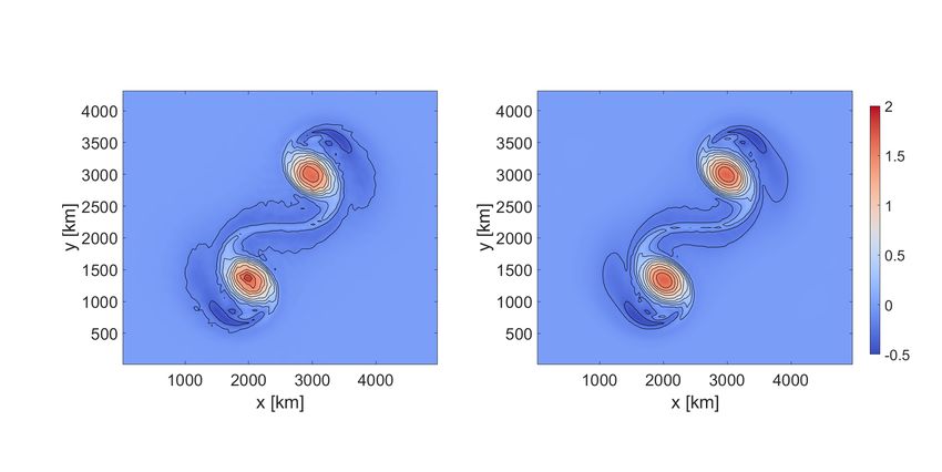
initial conditions to simulate the two co-rotating vortices for 2 days. In Figure 3, we show contour
plots of the potential vorticity (as defined in (3.7)) fields of the deterministic and stochastic
17Figure 3. Contour plots of the potential vorticity fields after 2 days for (left) one realization of a LU simulation
with homogeneous noise and (right) a deterministic run. The contour interval is 0.4 days−1 km−1 .
models. We observe that under the moderate noise with a0 as chosen above, the large-scale
structure of the stochastic system is similar to that of the deterministic run.
On the specific staggered grid as shown in Figure 2, the total energy of the shallow water
equations (A.1), for both deterministic and stochastic case, is approximated by
N
X 1 X 1 2 1 2
E(t) ≈ Di (t)|Ti | hik fik Vik (t) + g Di (t) |Ti |. (4.3)
2 2|Ti | 2
i=1 k=j,i− ,i+
As shown in Bauer and Gay-Balmaz (2019a), the proposed discrete variational integrator
(see Section 3.1) together with an iterative Crank-Nicolson time stepping method exhibits a
1st order convergence rate of the energy error with smaller time step size. This will allows us
immediately to simply include the stochastic terms to result in an Euler-Maruyama type time
integrator for stochastic systems (cf. Section 3.2).
In the present work, we consider the energy behavior of the deterministic scheme (i.e. the vari-
ational integrator) as reference, which is denoted as EREF (t) in the following. For the stochastic
RSW model, the Euler-Maruyama time scheme might lead to a different behavior with respect
to energy conservation when compared to the deterministic model. In order to quantify numeri-
cally the energy conservation of the RSW–LU, we propose to measure the relative errors between
the mean stochastic energy, denoted as ELU (t), and the reference EREF (t) by ELU (t)/EREF (t) − 1,
while using for both the same spatial resolution (see Table 1). This setup allows us to measure
the influence of the stochastic terms on the energy conservation relative to the deterministic
scheme. Figure 4 shows these relative errors for different time step sizes over a simulation time
of 2 days. As we can confirm from the curves, taking successively smaller time steps
∆t ∈ {1.7361 × 10⁻⁴ , 3.4722 × 10⁻⁵ , 1.7361 × 10⁻⁵ , 3.4722 × 10⁻⁶ , 1.7361 × 10⁻⁶ } (in days−1 )
results in smaller relative errors.
To determine more quantitatively the convergence rate of the stochastic scheme (relative to
the reference) with respect to different time step sizes, we defined the following global (in space
and time) error measure:
kELU (t) − EREF (t)kL2 ([0,T ])
4
ε(ELU ) = , (4.4)
kEREF (t)kL2 ([0,T ])
RT
where kf (t)kL2 ([0,T ]) = ( 0 |f (t)|2 dt)1/2 and T is set to 2 days. We determine for an ensemble
with 10 members such global errors in order to illustrate the convergence rate of each ensemble
1810 -6
relative error 10 -8
10 -10
10 -12
10 -14
10 -16
0 0.5 1 1.5 2
days
Figure 4. Evolution of the relative L2 errors between the energy of the mean RSW–LU and the reference, using
∆t (blue line), ∆t/10 (red line) and ∆t/100 (yellow line) respectively.
member and the spread between those rates. This spread is illustrated as blue shaded area in
Figure 5. The area centre is determined by the mean of the errors, and the dispersion of this
area is given by one standard derivation (i.e. 68% confident interval of the ensemble of ε(ELU )).
Besides, the minimal and maximal values of the errors of the ensemble are represented by the
vertical bar-plots. The blue line of Figure 5 shows that the convergence rate (w.r.t. various ∆t)
of the ensemble mean energy is of 1st order. This is consistent with the weak convergence rate
of order O(∆t) of the Euler-Maruyama scheme, cf. Section 3.3.
4.2 Viscous test case - ensemble prediction
Next, we want to show that our stochastic system better captures the structure of a large-
scale flow than a comparable deterministic model. To this end, we use a viscous test case and
heterogeneous noise.
The viscous test case we use is proposed by Galewsky et al. (2004) and it consists of a
barotropically unstable jet at the mid-latitude on the sphere. This strongly non-linear flow will
be destabilized by a small perturbation of the initial field, which induces decaying turbulence
after a few days. However, the development of the barotropic instability in numerical simulations
highly depends on accurately resolving the small-scale flow, which is particularly challenging for
coarse-grid simulations. For the same reason, the performance of an ensemble forecast system
in this test case is quite sensible to the numerical resolution. In the following, we demonstrate
that the RSW–LU simulation on a coarse mesh under heterogeneous noises, provides better
prediction of the barotropic instability compared to the deterministic coarse simulation, and
produces more reliable ensemble spread than the classical PIC simulation.
19You can also read