Modons on Tidally Synchronised Extrasolar Planets
←
→
Page content transcription
If your browser does not render page correctly, please read the page content below
Mon. Not. R. Astron. Soc. 000, 1–?? (yyyy) Printed 15 September 2021 (MN LATEX style file v2.2)
Modons on Tidally Synchronised Extrasolar Planets
J.
1
W. Skinner,1? J. Y-K. Cho,1,2,3 †
School of Physics and Astronomy, Queen Mary University of London, Mile End Road, London E1 4NS, UK
2 Department of Astrophysical Sciences, Princeton University, 4 Ivy Lane, Princeton, NJ, 08544,USA‡
3 CCA, Flatiron Institute, 162 Fifth Ave, New York, NY, 10010, USA §
Accepted yyyy mmm dd. Received yyyy mmm dd; in original form yyyy mmm dd
arXiv:2109.06568v1 [astro-ph.EP] 14 Sep 2021
ABSTRACT
We investigate modons on tidally synchronised extrasolar planets. Modons are highly dy-
namic, coherent flow structures composed of a pair of storms with opposite signs of vorticity.
They are important because they divert flows on the large-scale; and, powered by the intense
irradiation from the host star, they are planetary-scale sized and exhibit quasi-periodic life-
cycles – chaotically moving around the planet, breaking and reforming many times over long
durations (e.g. thousands of planet days). Additionally, modons transport and mix planetary-
scale patches of hot and cold air around the planet, leading to high-amplitude and quasi-
periodic signatures in the disc-averaged temperature flux. Hence, they induce variations of
the “hot spot” longitude to either side of the planet’s sub-stellar point – consistent with obser-
vations at different epoch. The variability behaviour in our simulations broadly underscores
the importance of accurately capturing vortex dynamics in extrasolar planet atmosphere mod-
elling, particularly in understanding current observations.
Key words: hydrodynamics – turbulence – methods: numerical – planets: atmospheres.
1 INTRODUCTION commonly-employed forcing and initialization generally produce a
large monolithic patch of nearly stationary hot area located east-
Modons are translating vortex dipole structures, consisting of two
ward of the sub-stellar point ∼2×10⁻³ MPa (Cooper & Showman
oppositely-signed patches of vorticity that form in the atmosphere
2005; Showman et al. 2008). The discrepancy between observa-
and ocean (Stern 1975). In atmospheric dynamics, modons play an
tions and simulations may arise because simulations thus far have
important role in establishing “blocking patterns” which prevent
lacked the required horizontal resolution (Skinner & Cho 2021).
weather or jet systems from moving through over a certain region.
Hence the simulations have not been able to accurately capture the
In a tidally synchronised planet atmosphere, a couplet of modons
dynamics of small-scales which influence the large-scale dynamics
forms – one composed of a pair of cyclones and the other composed
(e.g. modons and jets) through their non-linear interactions with
of a pair of anti-cyclones: cyclones (anti-cyclones) are storms char-
the large-scales. Accurately modelling these interactions is essen-
acterised by vorticity having the same (opposite) sense as the plane-
tial because dynamics serves as the core for other important at-
tary vorticity (e.g. Holton 2004). These modons are planetary-scale
mospheric processes such as radiative transfer, clouds, photochem-
in size, and they initially span across the equator (assuming zero
istry, and ionization.
obliquity for the planet). While both modons are spatially com-
pact and isolated, they generally interact strongly with each other In this paper, we describe the results from a set of high-
as well as other flow structures present in the atmospheres of the resolution simulations, which accurately capture the small-scale
synchronised planets because of the large interaction length-scale vortices (storms) and waves inherent in synchronised planet atmo-
(the Rossby deformation scale LR ) for the flow structures. spheres – hence, accurately represent large scale dynamics. Our
Currently, observations of hot-Jupiter atmospheres show large results are grounded in a series of extensive numerical convergence
variations in the longitudinal location of the “hot spot” as well as and parameter sensitivity studies with the code used in the present
the amplitude of spectral features (e.g. Grillmair et al. 2008; Zellem work (Polichtchouk and Cho 2012; Polichtchouk et al. 2014; Cho,
et al. 2014; Armstrong et al. 2017; Dang et al. 2018; Zhang et al. Polichtchouk & Thrastarson 2015; Skinner & Cho 2021). We find
2018; Jackson et al. 2019); see also Cho et al. (2019) for a re- that tidally synchronised planet atmospheres contain a large num-
cent review. However, atmospheric flow simulations that use the ber of intense storms, that span a wide range of sizes – including the
planetary-scale. Significantly, these planetary-scale storms greatly
influence the large-scale spatial distribution and temporal variabil-
?
ity of hot, as well as cold, regions over the planet. These storms
E-mail: j.w.skinner@qmul.ac.uk
† E-mail: jcho@flatironinstitute.org and their motions lead to signatures that may be observable and,
‡ on leave from Queen Mary University of London therefore, important for interpreting and guiding current and future
§ present address observations (Cho, Skinner & Thrastarson 2021).
© yyyy RAS
2       J. W. Skinner & J. Y-K. Cho
      The outline of this paper is as follows. In Section 2, we de-                     hyper-dissipation (see e.g. Cho and Polvani 1996a; Thrastarson &
scribe the numerical model we use, how it is set up for the simula-                     Cho 2011; Polichtchouk and Cho 2012); C = (2/Rp2 )p is a term
tions described in this work and linear theory relevant for the non-                    that compensates the damping of uniform rotation by Dv (see e.g.
linear solutions obtained with the model. In Section 3, we describe                     Polichtchouk et al. 2014); ρ(x, t) is the density; cp is the constant
the transient and persistent solutions that arise when the aforemen-                    specific heat at constant pressure; and, q̇net (x, t) is the net diabatic
tioned setup, which is commonly-employed in extrasolar planet                           heating rate.
studies, is used. We emphasize that the primary focus of this paper                           Equations (1) are closed by the equation of state for an ideal
is on the flow and its associated temperature distributions: results                    gas, p = ρRT , where R is the specific gas constant. A useful vari-
from a comprehensive study of numerical convergence and accu-                           able is the potential temperature, Θ(x, t) ≡ T (Pref /p)κ , where
racy (which includes the high resolution and dissipation order em-                      pref is a constant reference pressure and κ ≡ R/cp ; for example,
ployed in this work) is reported in Skinner & Cho (2021), and anal-                     Θ is materially conserved when q̇net = DT = 0. The boundary con-
ysis incorporating radiative transfer, chemistry, and aerosols will                     dition for the equations is “free-slip” (i.e. Dp/Dt = 0) at the top
be described elsewhere. In particular, here we focus on the quasi-                      and bottom p-surfaces; note that the top and bottom boundaries are
periodic behaviour of modons and their effects on the flow and tem-                     material surfaces, across which no mass is transported. With this
perature fields. Significantly, this behaviour produces discernible                     boundary condition, the equations permit the full range of large-
signatures in disc-averaged temperature fluxes. In Section 4, we                        scale motions for a stably-stratified, un-ionized atmosphere – with
conclude by briefly summarising this work and discussing its im-                        the exception of sound waves: sound waves are filtered out from the
plications for extrasolar planet circulation modelling and observa-                     full compressible hydrodynamics equations2 via the combination
tions.                                                                                  of the hydrostatic balance condition, expressed by equation (1b),
                                                                                        and the free-slip boundary conditions at the top and bottom. How-
                                                                                        ever, the results presented in this study (e.g. the emergence of dy-
2     METHODOLOGY                                                                       namic modons) also apply to simulations solving the full Navier-
                                                                                        Stokes (non-hydrostatic) equations employing a similar physical
2.1    Governing Equations                                                              setup, since the speed of fast gravity waves admitted by both the
The governing equations, numerical model, and simulation setup                          hydrostatic and non-hydrostatic equations are close to the speed of
used in this paper are the same as in Skinner & Cho (2021) and                          the sound wave (see Table 1).
Cho, Skinner & Thrastarson (2021). We reproduce the key points
of the equations and model here for the reader’s convenience. As
in many past works, we solve the traditional primitive equations                        2.2   Numerical Model
(see e.g. Salby 1996) in x = (λ, φ, p) coordinates, representing                        We solve equations (1) and (2) numerically using the pseudospec-
(longitude, latitude, pressure) in this work. The equations read:                       tral code, BOB (Rivier, Loft & Polvani 2002; Scott et al. 2004).
 Dv                       u                                                           BOB is a highly-accurate “dynamical core” of a general circulation
        = −∇p Φ −              tan φ + f k × v + Dv              (1a)                   model (GCM). GCMs are typically used in atmospheric dynam-
 Dt                         Rp
∂Φ              1                                                                       ics studies and climate modelling of the Solar System planets. But,
        = −                                                     (1b)                    BOB has been rigorously tested and validated under the numer-
 ∂p             ρ
                                                                                        ically stringent conditions typical of hot-Jupiters; see, for exam-
 ∂ω
        = −∇p · v                                                (1c)                   ple, Polichtchouk and Cho (2012), Polichtchouk et al. (2014), Cho,
 ∂p                                                                                     Polichtchouk & Thrastarson (2015) and Skinner & Cho (2021).
 DT           ω       q̇net                                                                   BOB solves the equations in the “vorticity-divergence and po-
        =          +         + DT ,                             (1d)
 Dt          ρ cp       cp                                                              tential temperature” form3 . In this form, equations (1) are more
where D/Dt ≡ ∂/∂t + v · ∇p + ω∂/∂p is the material deriva-                              suited to the spectral transform method (see e.g. Orszag 1970;
tive; t is the time; v = (u, v) is the (eastward, northward) ve-                        Eliasen et al. 1970; Canuto et al. 1988), which offers superior
locity (in a frame rotating with rotation rate Ω) on a constant p-                      convergence properties compared to the traditional (e.g. finite dif-
surface; ω ≡ Dp/Dt is the “vertical” pressure velocity in the                           ference) schemes (e.g. Boyd 2000; Durran 2010). BOB is essen-
rotating frame; Rp is the planetary radius, which is fiducially set                     tially a multi-layer extension of the 1-layer codes used in the stud-
to be at p = 0.1 MPa; k is the unit vector in the local vertical                        ies of Solar System giant planets by Cho and Polvani (1996a,b)
direction; ∇p is the horizontal gradient on a constant p-surface;                       and extrasolar system giant planets by Cho et al. (2003, 2008).
Φ(x, t) = gz(x, t) is the geopotential, where g is the constant sur-                    The time integration of the equations in all of these codes is per-
face gravity at z = Rp with z the vertical distance above Rp ;                          formed using a second-order accurate, leap-frog scheme with a
f (φ) = 2Ω sin φ is the Coriolis parameter, the projection of the                       small amount of Robert–Asselin filter applied to suppress the com-
planetary vorticity vector 2Ω onto k; the direction of Ω orients                        putational mode arising from the scheme (Robert 1966; Asselin
north; T (x, t) is the temperature; Dχ , for χ ∈ {v, T }1 , is given by                 1972). The time-step size ∆t in all the simulations are such that the
                                                                                        Courant-Friedrichs-Lewy (CFL) number (e.g. Strikwerda 2004;
Dχ = ν2p (−1)p+1 ∇p2p + C χ ,

                                                                     (2)                Durran 2010) is well below unity – typically < 0.3.
where ν2p is the constant dissipation coefficient; p ∈ N, where                               For each p-surface, the code transforms the equations to the
N = {0, 1, 2, . . . }, is the order of the dissipation (not to be con-                  spectral space with a “triangular truncation” – i.e. up to N = M ≡
fused with the pressure p) with p > 1 instantiations known as
                                                                                        2  Although sound waves are not admitted, the primitive equations are still
1  As in Skinner & Cho (2021), { · , · , . . .}, [ · , · ] and ( · , · , . . .) carry   compressible, as Dρ/Dt 6= 0; see equation (1c).
their usual meanings in this paper – i.e. set, (closed) interval and tuple,             3 the curl and divergence of equation (1a), along with equation (1d) in

respectively.                                                                           terms of the potential temperature

                                                                                                                                 © yyyy RAS, MNRAS 000, 1–??
Modons on Tidally Synchronised Extrasolar Planets                           3

Table 1. Physical, Numerical, and Scale Parameters: (a) based on cp ;
                                                                                    the use of p  1 (e.g. Cho and Polvani 1996a; Boyd 2000; Durran
(b)for {H2 , He}; (c) at p = 0.1 MPa; (d) at p = 1 KPa                              2010; Skinner & Cho 2021).
                                                                                          Since our goal is to follow the evolution of highly dynamic
 Planetary rotation rate               Ω           2.1×10⁻⁵         s−1             and minimally dissipated flow structures over a long duration, we
 Planetary radius                      Rp          108              m               use p = 8. The role of Dχ is to limit dissipation to the small-scales
 Surface gravity                       g           10               m s−2           and to provide a conduit for energy and enstrophy cascade that pre-
 Specific heat at constant p           cp          1.23×10⁴         J kg−1 K−1      vent the simulation from “blowing up”. As has been demonstrated
 Specific gas constant(a,b)            R           3.5×10³          J kg−1 K−1      in Skinner & Cho (2021), p > 8 is required at the currently prac-
                                                                                    tical resolutions to adequately capture the full range of behaviours
 Initial temperature(c)                Tm          1600             K               exhibited in the flow. Using a lower p, especially at low resolu-
 “Equil.” sub-stellar temp.(c)         Ted         1720             K               tion, can dissipate large-scale structures – even the n = 2 mode
 “Equil.” anti-stellar temp.(c)        Ten         1480             K               structures, important in the present work. Other than the very weak
 Thermal relax. time (d)               τth         ≈ 105            s               Robert–Asselin filter to separate out the computational mode aris-
 Pressure at top                       ptop        0                MPa
                                                                                    ing from the leapfrog scheme (Thrastarson & Cho 2011), no other
 Pressure at bottom                    pbot        [0.1, 10]        MPa
 Pressure w/o forcing                  p0          >1               MPa
                                                                                    numerical dissipators, drags, fixers, stabilisers or filters are used in
                                                                                    performing the simulations, as they are not necessary in our code.
 Truncation wavenumber                 T           [21, 682]                              Vertically, the domain is decomposed into L ∈ Z+ uniformly-
 Number of levels (or layers)          L           [3, 1000]                        spaced points or layers in the p-coordinate. Along this direction,
 Max. sectoral wavenumber              M           =T                               a second-order finite-difference scheme is used – as is common in
 Max. total wavenumber                 N           =T                               codes solving equations (1) (e.g. Durran 2010). Given the range,
 Dissipation operator order            p           [1, 8]                           p ∈ [ptop , pbot ], the dynamically active levels pk for k ∈ [1, L] are
 Viscosity coefficient                 ν2p         (see text)       m2p s−1         located at
 (Hyper)dissip. wavenumber             nd(2p)      (see text)
                                                                                                  1 h pbot − ptop i
                                                                                    pk = k −                          .                                  (6)
 Vertical length scale                 H           ∼ RTm /g         m                              2          L
 Horizontal length scale               L           & Rp /20         m
 Maximum jet speed                     U           & 2×10³          m s−1
                                                                                    As already mentioned, the bounding surfaces, ptop and pbot , are
 Sound speed(c)                        cs          ≈ 2.8×10³        m s−1           not dynamically active; but, they enforce the boundary conditions.
 Dissipation time-scale                τd          ∼ 2×10⁵          s               Note that many studies employ a log(p)-spacing (e.g. Liu & Show-
 Brunt-Väisälä frequency            N           ∼ 2×10⁻³         s−1             man 2013); but, they tend to solve the equations in a uniform
 Rossby number                         Ro          ≡ U /(ΩL)                        p-coordinate, which introduces a numerical complication (Cho,
                                                        √
 Froude number                         Fr          ≡U√/ gH                          Polichtchouk & Thrastarson 2015). This difference in the vertical
 Rossby deformation scale              LR          ≡ gH/Ω           m               spacing, however, does not alter the main results of the present pa-
                                                                                    per.

T wavenumbers retained in the Legendre expansion,
                 N
                 X         M
                           X                                                        2.3   Simulation Setup
ξ(λ, µ, t) =                      ξnm (t) Ynm (µ, λ),       |m| 6 n ,         (3)   The physical parameters and their values for equation (1) are shown
                 n=0       m=−M
                                                                                    in Table (1). The parameter values are representative of the tidally
where ξ is an arbitrary scalar field; µ ≡ sin φ; n ∈ N and m ∈ Z are                synchronised extrasolar giant planet HD209458b. Note that the val-
the total and sectoral wavenumbers, respectively; (N, M ) ∈ N2 ;                    ues in the table are identical to those used in many hot-Jupiter mod-
Ynm (λ, µ) ≡ Pnm (µ) eimλ are the spherical harmonic functions;                     elling studies (see e.g. Thrastarson & Cho 2010; Skinner & Cho
and, Pnm are the associated Legendre functions. The set {Ynm } are                  2021). This facilitates equatable comparisons. Note also that, due
the eigenfunctions of the spherical Laplacian operator:                             to the free-slip boundary condition at pbot , the results in this paper
                                                                                  are relevant to telluric planets with a solid or liquid surface, away
                 n(n + 1)
∇2 Ynm = −                   Ynm ,                               (4)                from their boundary layers. 4
                    Rp2
                                                                                         For the thermal forcing of the planet’s atmosphere, we adopt
where                                                                               a commonly utilised scheme that has been implemented in many
    1

                  ∂

                                        ∂

                                                     1   ∂2
                                                                                   past studies (see e.g. Showman & Guillot 2002; Cho et al. 2003;
  2                               2
∇ = 2                      1−µ                  +                   .         (5)   Cooper & Showman 2005; Cho et al. 2008; Showman et al. 2008;
   Rp            ∂µ                    ∂µ         1 − µ ∂λ2
                                                       2
                                                                                    Menou & Rauscher 2009; Rauscher & Menou 2010; Thrastar-
The {Ynm } constitutes a complete, orthogonal expansion basis (e.g.                 son & Cho 2010; Heng et al. 2011; Liu & Showman 2013; Cho,
Byron & Fuller 1992). Note that, when p = 1, equation (2) reduces                   Polichtchouk & Thrastarson 2015; Skinner & Cho 2021). In this
to the Laplacian operator acting on χ, modulo C. Note also that a                   idealised setup, an atmosphere which is initially at rest is driven
representation in spectral space with a truncation wavenumber T                     by a thermal relaxation to a prescribed “equilibrium temperature”.
is transformed to a Gaussian grid in physical space with approx-                    Specifically, q̇net /cp in equation (1d) is set to be −(T − Teq )/τth ,
imately (3T, 3T/2) points in the (λ, φ)-direction. However, the                     where Teq = Teq (λ, φ, p) is the equilibrium temperature and
Gaussian grid should not be directly compared with the grid of a
finite-difference (or other grid-based) methods, as the former grid
is effectively equivalent to a much higher resolution than a finite-
difference grid with the same number of points. This is due to the                  4 Here, by ‘telluric’ we mean a planet with a solid lower boundary (and
pseudospectral method’s accuracy and convergence properties and                     smaller radius).

© yyyy RAS, MNRAS 000, 1–??
4      J. W. Skinner & J. Y-K. Cho
τth = τth (p) is the radiative “cooling” time 5 ; more precisely, it
is the thermal relaxation time. The Teq distribution is specified as:
          (
            Ten (p) + ∆T (p) cos λ cos φ,      day-side
Teq =                                                             (7)
            Ten (p),                           night-side .
Here Ten is the equilibrium temperature at the night-side, which
is uniform at each p. In contrast, the day-side equilibrium temper-
ature is not uniform, with Ten + ∆T ≡ Ted (p) the temperature
at the sub-stellar point, (λ, φ) = (0◦ , 0◦ ), for ∆T ≡ Ted − Ten .
The specified, simple profiles {Tref , ∆T, Ten , Ted , τth } all depend
only on p and crudely represent the effects of irradiation from the
planet’s host star on the dynamics. The profiles are shown in Fig. 1.
      In Fig. 1, each of the profiles are piece-wise continuous func-
tions of p that span the vertical range, p = [10−5 , 101 ] MPa. It
is important to note that for this setup the strength of the thermal
forcing is flow independent, which is not realistic (especially when
τth . τad , where τad ≡ L/U with L = πRp is the advective
time). Moreover, the unknown τth (p) is chosen so that the forcing
strength is monotonic and strongest at the top of the atmosphere
and goes to zero at p = 1 MPa; at p > 1 MPa, forcing is not ap-
plied. Note that quantitative aspects of the flow are affected by the
chosen profiles (as well as by the initial flow state) – as empha-
sized repeatedly in the past (Cho et al. 2008; Thrastarson & Cho
2010; Cho, Polichtchouk & Thrastarson 2015; Cho et al. 2019).
Another feature to note is the zonal6 asymmetry of Teq , which is re-
sponsible for generating the main (zonally-asymmetric) flow struc-
ture discussed in this paper: the cyclonic and anti-cyclonic modon             Figure 1. Temperature (a) and relaxation time (b) profiles used in the New-
pair. “Deeper asymmetry” about the terminator in Teq , such as the             tonian cooling scheme. (a) Blue solid line shows the reference temperature
cos λ distribution extending to the nightside (e.g. Thrastarson &              Tref , which is the initial temperature (uniform at each p). The accompa-
Cho 2010; Showman & Polvani 2011), leads to stronger asymme-                   nying black dashed lines show the equilibrium temperature profiles, Ted at
try in the flow. The effects of the asymmetry are discussed more in            the sub-stellar point (right) and Ten at the anti-stellar point (left); the latter
detail in section 3.                                                           temperature is a constant over the entire night-side at each p-level. The red
      Fig. 2 shows three useful profiles derived from the tem-                 dotted line is the equilibrium temperature difference, ∆T ≡ Ted − Ten .
                                                                               (b) The thermal relaxation time τth is roughly proportional to p/Tref   4 in the
perature profiles presented in       Fig. 1: level meanR k+1atmospheric                                  −3
                                 R k+1                                         sloping region (p = [10 , 1] MPa) and uniform above and below (τth is
scale height, H(p) ≡ (R k T d ln p) / (g k d ln p), in
                                                                               a constant at each p-level). Outside the sloping region, τth is very short at
units of Mm (left); potential temperature, Θ(p) ≡ T (10/p)κ ,
                                                                               the top (τth  τad at p 6 10−3 MPa) and long at the bottom (τth  τad
in units of K (centre); and, Brunt-Väisälä frequency, N (p) ≡               at p > 1 MPa).
[−ρg 2 (d ln Θ/dp)]1/2 , in units of 10−3 s−1 (right). The black
lines correspond to the initial profile Tref ; and, the blue and red
lines correspond to equilibrium profiles Teq of the anti-stellar and           default. However, the temperature T and pressure p are given the
sub-stellar points, respectively. The temperature profiles lead to             units of K and MPa, respectively for easier comparison with past
abrupt changes in the vertical Θ gradients – i.e. jumps in the ba-             simulation and observatonal studies. Hence, for all the simulations
sic stratification – as seen in the Brunt-Väisälä frequencies. Note,        discussed in this paper, ptop = 0 while pbot ∈ {0.1, 1.0, 10}. Note
the blue profile nearly vanishes at p ≈ 10−4 MPa, but it is still              that a range of simulation domains are chosen to explore the robust
positive. It is also an artefact of the unrealistic discontinuity in the       features, for the given setup. Appropriate p-levels for the top and
corresponding temperature profile. Formally, the hydrostatic bal-              bottom of the simulations are currently unknown (Cho et al. 2008).
ance condition restricts the validly of equations (1) to the stably-
stratified radiative region p <
                              ∼ 10 MPa, which overlies an unstably-
                                      2
stratified convective region p >∼ 10 MPa. The exact transition level           2.4   Linear Theory
between the stable and unstable region is uncertain, and likely lat-
                                                                               Before embarking on the full non-linear solutions, a brief discus-
erally dependent.
                                                                               sion of linear theory is instructive. Under the barotropic (vertically
      From hereon, the planetary radius Rp and rotation period τ
                                                                               aligned) and isochoric (constant density) assumptions, equation (1)
(≡ 2π/Ω = 3.025×10⁵ s) are used as the length and time scales,
                                                                               reduces to the shallow-water equations for a single layer of fluid
respectively – whenever confusion is not engendered. That is, ν2p is
                                                                               (Pedlosky 1987). Here we confine our attention to a tangent plane
given in the units of Rp2p τ −1 and n is given in the units of Rp−1 , by
                                                                               situated at the equator (φ = 0), known as the equatorial β-plane
                                                                               approximation (e.g. Matsuno 1966; Gill 1980; Wu, Sarachik & Bat-
5                                                                              tisti 2001):
   The “spin up” time varies with depth and vertical resolution in all simu-
lations, but it is around 10 planetary days for the pbot ∼ 0.1 simulations.    Dv
                                                                                       =     −g∇h − βyk × v ,                                               (8a)
For pbot > 1, “spin up” time is undefined (Mendonça 2020).                    Dt
6 “Zonal” refers to eastward and “meridional” refers to northward (and
                                                                               Dh
sometimes more loosely east–west and north–south, respectively).                       =     −h∇·v ,                                                       (8b)
                                                                               Dt

                                                                                                                            © yyyy RAS, MNRAS 000, 1–??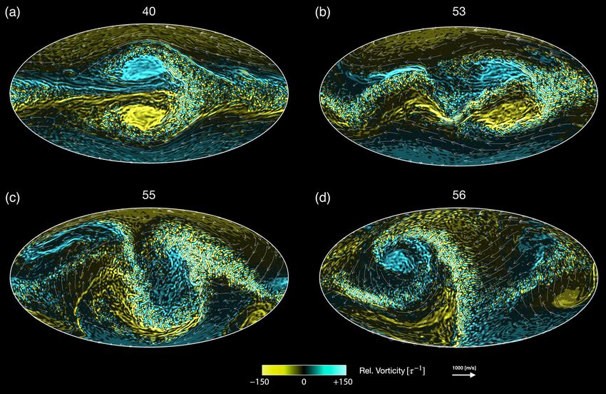
Modons on Tidally Synchronised Extrasolar Planets                                        5

Figure 2. Level mean scale height H(p) in units of Mm (left), potential temperature Θ(p) in units of K (centre), and Brunt-Väisälä frequency N (p) in units
of 10−3 s−1 (right) for the temperature profiles in Fig. 1. The black lines correspond to the initial profile Tref ; and, the blue and red lines correspond to
equilibrium profiles of the anti-stellar and sub-stellar points (Ten and Ted ), respectively. The temperature profiles lead to abrupt changes in the vertical Θ
gradients – i.e. jumps in the basic stratification – as seen in the Brunt-Väisälä frequencies. In the latter, the blue profile nearly vanishes at p ≈ 10−4 MPa, but
it is still positive.

where now D/Dt ≡ ∂/∂t + v · ∇ with ∇ ≡ (∂/∂x, ∂/∂y);                                  Ro ≡ U/(βL2 ), we obtain:
v = (u, v) ∈ R2 , where u(x, t) is the zonal velocity and v(x, t)
                                                                                       ∂u        ∂h
is the meridional velocity; h(x, t) is the fluid thickness; β ≡                           − vy +              =    0,                                            (9a)
                                                                                       ∂t        ∂x
df /dy |y=0 = 2Ω/Rp is the meridional gradient of the Corio-
                                                                                       ∂v        ∂h
lis parameter at the equator; and, k is again the unit vector in the                      + uy +              =    0,                                            (9b)
                                                                                       ∂t        ∂y
vertical direction. With the boundary condition, y → ±∞, the dy-
namics is effectively confined in the equatorial region because of                     ∂h   ∂u    ∂v
                                                                                          +    +              =    0.                                            (9c)
the finiteness of LR ; hence, the equatorial beta plane acts like a                    ∂t   ∂x    ∂y
wave guide along the equator, with a number of different zonally                      From this, we can find a general solution for linear modes at the
propagating waves that are confined in the meridional direction and                   equator, by eliminating u and h and obtaining an equation for v:
divided into fast and slow types. Importantly, equatorial waves in
equations (1) have the same horizontal structure as those admitted                     ∂  2          ∂2 v  ∂v
                                                                                          ∇ v − y2 v − 2 +      = 0.                                             (10)
by equations (8). However, we stress that the use of β-plane model                     ∂t             ∂t     ∂x
here is used to motivate the explanation for the initial formation                    Now, expanding v in a series in theP
                                                                                                                         Hermite polynomial basis ϕl
of the modon (only). The Matsuno-Gill solution for the equatorial                     (Abramowitz & Stegun 1965), v = l vl (x, t)ϕl (y), and using
β-plane (e.g. Showman & Polvani 2011), for example, does not
formally and realistically apply to hot synchronised planet atmo-                      d2 ϕ l
                                                                                              + (2l − y 2 + 1) ϕl = 0                                            (11)
spheres7 because of the following (Cho et al. 2019): i) large merid-                   dy 2
ional scale of the modons invalidates the tangent plane approxima-                    gives the following equation:
tion; ii) a pre-existing, strongly time-varying background flow and
temperature field due to dynamic modons and other storms, which                        ∂ h ∂2 vl                ∂2 vl i ∂vl
                                                                                                 − (2l + 1)vl −        +    = 0.                                 (12)
preclude classical eddy–mean flow interaction theory (e.g. Vallis                      ∂t ∂x2                   ∂t2      ∂x
2017); iii) incompressible (small Mach number) and homogeneous-                       This leads to
layer (unconstrained LR ) assumptions of the shallow-water model;
and, iv) hot-Jupiters are not expected to have a linear Rayleigh drag.                ∂3 v̂l                  ∂v̂l
                                                                                              + (k2 + 2l + 1)      − ikv̂l = 0 ,                       (13)
      Upon non-dimensionalising equations (8) with the scaling,                        ∂t3                     ∂t
(v, x, t) → (U v, Lx, τs t), where U , L, and τs ≡ L/U are the                        where v̂l (k, t) = vl (x, t) eikx dx + c.c. is the Fourier transform
                                                                                                          R
characteristic speed, length, and time scales, respectively, and then                 of vl . The general solution for equation (13) is:
linearising the equations to zeroth-order in the Rossby number,
                                                                                              3
                                                                                              X
                                                                                      v̂l =         vα (k) e−iωα t ,                                             (14)
                                                                                              α=1

                                                                                      where ωα for α = 1, 2, 3 are the three roots of the dispersion equa-
                                                                                      tion:
                                                                                       3
                                                                                      ωα − (k2 + 2l + 1)ωα − k = 0 .                                             (15)

                                                                                      Here, the lowest value of ωα at a given (k, l) corresponds to a wave
7 particularly to explain the supersonic, zonally-symmetric, equatorial jet           with westward propagation. This is the equatorial Rossby wave, im-
which develop after a long time in low-resolution simulations                         portant for the large-scale structure in our work. Note that l gives

© yyyy RAS, MNRAS 000, 1–??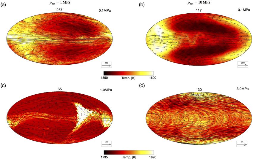
6       J. W. Skinner & J. Y-K. Cho

Figure 3. Velocity (vectors) and height perturbation (contours) distributions
for the equatorial Rossby wave with (k, l) = (1, 1), illustrating the hor-
izontal structure of the dominant flow pattern in this paper (e.g. bottom
p-level of Fig. 4). Note the different scalings in the x and y directions,
appropriate for the dynamics under discussion. For the contours, negative
(positive) values are full (dashed); under geostrophy, height and vorticity
perturbation fields are locally (and at the equator) related by the Laplacian
and opposite signs in spectral amplitude.                                       Figure 4. Relative vorticity surfaces ζ(λ, φ, p) = ±3 (in units of τ −1 and
                                                                                at τ −1 intervals, with positive values in red and negative values in blue), at
                                                                                t = 0.25 (in units of τ ) from a T341L20 simulation: the dissipation order is
the number of nodes in the meridional direction for v. The approx-              p = 8, viscosity coefficient is ν16 = 1.5 × 10−43 (in units of Rp2p τ −1 ),
imate solution to equation (15) is                                              and time-step size is ∆t = 4×10⁻⁵ (in units of τ ). Black arrows show bulk
                                                                                velocity (∼ 500m/s). The section of the atmosphere shown is centred on the
                 k                                                              sub-stellar point (λ, φ) = (0, 0) with vertical range p ∈ [0, 0.1] (in units
ωl (k) =                .                                               (16)
            2l + k2 + 1                                                         of MPa). When the simulations are initialised as described in Section 2.3
     The velocity and height perturbation distributions for the                 (i.e. baroclinic thermal forcing applied to atmosphere at rest), a “hetonic
equatorial Rossby wave with (k, l) = (1, 1) from equation (15) are              quartet” forms at the sub-stellar point; a second quartet forms at the night-
                                                                                side. This baroclinic structure cannot be captured by a barotropic model
shown in Fig. 3. The figure illustrates the horizontal structure of
                                                                                (e.g. shallow-water model in Section 2.4). The quartet is composed of two
the dominant flow pattern in this paper, a modon pair. We note that             oppositely-signed hetons, which here is anti-symmetric across the equator
Rossby waves generally have much lower phase velocities than in-                and separated in latitude by φ ∼ 80◦ . Each heton is a columnar structure
ertia–gravity waves. In addition, in the long-wave part of the wave             composed of a pair of similar strength and oppositely-signed vortices at
spectrum, there is a well-pronounced gap between inertia-gravity                different p levels (which here are tilted in longitude by λ ∼ 20◦ ). The
waves and the rest of the spectrum. In the next section, we show                heton quartet is a transient feature of the employed setup and is broken up
how such a structure is modified in its morphology and dynamical                by a strong vertical shear with the upper part of the atmosphere accelerating
behaviour under full non-linearity and forcing at high resolution.              to a fast equatorial jet. The formation is independent of the location of the
                                                                                pbot considered – i.e. pbot ∈ [0.1, 10].

3     RESULTS                                                                        As seen in Fig. 4, this early time flow structure is composed
3.1    Initial Structures                                                       of a pair of hetons – i.e. a “hetonic quartet” (Kizner 2006). This
                                                                                hetonic quartet is a vortical quadrupole which forms in response to
Fig. 4 presents surfaces of relative vorticity (ζ = ±3, in units of τ −1        the specified thermal forcing. The two hetons, as a pair, straddle the
and at τ −1 intervals), centred at the sub-stellar point (λ = 0, φ = 0),        equator and their centres are separated by a latitudinal distance of
at t = 0.25. The red and blue surfaces correspond to positive- and              ∼ 80◦ . Both hetons are slightly tilted in the longitudinal direction,
negative-valued surfaces, respectively. The overall structure seen in           with the top vortical structure offset longitudinally by ∼ 20◦ from
the figure is a pair of vortex columns, each with opposite signs of ζ           the bottom vortical structure. Also, both hetons are cyclonic8 in the
in the vertical direction. The vortex columns form almost immedi-               p . 2.5 × 10⁻² region and anti-cyclonic in the p & 2.5 × 10⁻²
ately after the start of the simulations and then quickly (within a few         region. Note that the p-level where the vorticity inversion occurs
τ ’s) evolve to a simpler structure, as described below. In oceanog-            depends on the extent of the simulation’s vertical domain (e.g. at
raphy, such columnar structures are known as “hetons” (Hogg &                   a deeper level for larger domain range). Note also that, in addition
Stommel 1985). Hetons are generated as a direct response to the                 to the heton quartet shown, a weaker and oppositely-signed heton
applied thermal forcing and potential vorticity (e.g. Pedlosky 1987)            quartet forms near the anti-stellar point; hence, there are actually
conservation, which is valid for this setup at early times and wher-            two (anti-symmetric) hetonic quartets – i.e. a “hetonic octet”. The
ever the flow is in equilibration with the applied thermal forcing.
The snapshot shown is from a T341L20 resolution simulation with
a vertical domain range of p ∈ [0, 0.1] and uniformly-spaced layers             8  Cyclonicity is defined according to the sign of ζ · Ω: the sign is positive
of ∆p = 5×10⁻³ thickness.                                                       for cyclones and negative for anti-cyclones.

                                                                                                                           © yyyy RAS, MNRAS 000, 1–??
Modons on Tidally Synchronised Extrasolar Planets 7
night-side hetons are larger in areal extent laterally; this is due to ric; this is in contrast with nearly all simulations in the past em-
the specified thermal forcing, which consists of relaxing the night- ploying the same setup with lower resolution and/or viscosity order
side temperature field to a uniform distribution that is much cooler (e.g. Liu & Showman 2013). Likewise for the unstable fronts; high-
than the day-side. Note that the octet formation is independent of resolution is required to capture this important source of medium-
the domain p-range considered in this work, from [0, 3×10⁻² ] to scale storms (Cho et al. 2003; Cho, Skinner & Thrastarson 2021;
[0, 20]. Skinner & Cho 2021). As for the planetary-scale storms, the most
Overall, both quartets are strongly barotropic but quickly be- generic state is a vortical quadrupole (at a given p-level), of which
come baroclinic (vertically tilted) as the thermal forcing accelerates at least one is a coherent modon (Fig. 5, and see also Figs. 6 and 8).
the flow at the top of the domain. As early as t = 1, the night- In general, there are two coherent modons, one composed of a pair
side quartet migrates to the day-side and the two quartets interact of cyclones and the other composed of a weaker pair of anticy-
strongly with each other at the eastern terminator. This results in in- clones, as already mentioned. In the figure, the storms compris-
tense baroclinic fronts that sweep across the eastern to western ter- ing the cyclonic modon are separated meridionally by a centre-to-
minators, from the low latitude to the pole, and in both the northern centre distance of ∼ πRp : the storms of the anticyclonic modon are
and southern hemispheres (the fronts, at a later time, can be seen much less conjoined and located closer to the poles. Additionally,
in Fig. 5). Significantly, the fronts undergo shear instability and act the cyclonic modon is generally shrouded by a sharp front to its
as sources of small-scale vortices (storms): wind speeds parallel to east and a trailing Rossby wave mostly to its west (seen as undula-
the fronts are already high, averaging ∼4.5 (i.e. ∼1500 m s−1 ) at tions along fronts propogating westward from the cyclonic modon
p < 5 × 10⁻² . In general, sharp fronts play a seminal role in hot in Fig. 5b), both of which generate copious small-scale storms and
exoplanet atmospheric dynamics. For example, capturing the front gravity waves. This is part of the “geostrophic adjustment” process
at the early time (or any other time later) leads to a subsequent of a modon (e.g. Lahaye & Zeitlin 2012). The multiple flow states
evolution which is markedly different than when not captured. The will be described separately in more detail later.
initially strong baroclinicity, eventually shears off the top of the Broadly, the flow features described above are seen at essen-
heton until like-signed vortical structures vertically align; this leads tially all the p-levels. Unlike the transient hetons described above,
to a strongly barotropic structure overall, dominated by the mod- neither of the cyclonic or anticyclonic modons in the figure changes
ons which grew in strength upward from the bottom. Thus, hetons its cyclonicity throughout the simulation. Modons are generally
are transient structures: they may also form at later times but are present near the top of the modelled atmosphere (Fig. 5a), although
weaker and more short-lived, due to the ambient flow conditions it is less prominent than at higher p-level (Fig. 5b): this is because
(which is not at rest). of the stronger anisotropic turbulence at the top. Nevertheless, jets
and fronts are both greatly influenced by the modons, independent
of p. In particular, when the cyclonic modon is positioned near the
3.2 Modon Pairs and Other Storms sub-stellar point the equatorial jet generally steepens, undulates and
Fig. 5 presents the main result of this paper: given the idealised then breaks on a time-scale of ∼3 planetary days. This strongly
setup of a tidally synchronised exoplanet as described above, a non-linear behaviour is caused by the oscillation and rotation of
pair of planetary-scale, strongly-barotropic modons is a generic the storms (that comprise the cyclonic modon) about their equi-
solution to equation (1). Under the applied forcing, a pair of mod- librium positions. Note also how the two constituent storms have
ons (cyclonic and anti-cyclonic) forms near the planet’s sub-stellar entrained small-scale storms from the breaking jet into their cores
point (λ = 0, φ = 0) and the anti-stellar point (λ = 180, φ = 0). (e.g. Fig 5a), thus mixing low-latitude air (and temperature) into
Both modons straddle the equator, but the night-side modon (anti- the mid-latitudes.
cyclonic) is always weaker than the day-side modon (cyclonic), Each modon forms out of an initial hetonic quartet, which
when they first form. The cyclonic modon can be clearly seen in strengthens upward in time from the lower vortex after the tops of
the figure, which shows the ζ-field at t = 100 – well after the ini- the original hetons are sheared away (as described in Section 3.1).
tial transient behaviour (generally lasting less than ∼10 planetary The first separation can occur as early as t = 5, resulting in chaotic
days). The resolution of the simulation in the figure is T682L20; mixing in the top region of the modelled atmosphere very quickly.
the dissipation order is p = 8; the viscosity coefficient is ν16 = Despite the meridional symmetry imposed by the initial and forcing
2.3×10−48 ; the time-step size is ∆t = 2×10⁻⁵ ; and, the extent of conditions, the flow and mixing break this symmetry early on. The
the vertical domain is p ∈ [0, 0.1]. The two levels presented, which zonal symmetry is also broken early on, even before the zonally
are from near the top and bottom of the simulation domain, show asymmetric forcing builds up its strength (recall the short relaxation
the strongly barotropic structure of the modon. Note that there is time τth ). Both the modon and the front radiate large-amplitude
no ζ inversion between the p levels shown in Fig. 5. We have per- gravity waves as well as induce formation of small-scale storms.
formed an extensive convergence assessment with the present setup The anti-cyclonic modons, which are less visible in Fig. 5, also ra-
and have verified that the features and behaviours presented in this diate and generate small-scale structures, but these structures are
paper are qualitatively robust at, or above, T341 horizontal resolu- weaker and more diffused.
tion with ∇16 hyper-viscosity (Skinner & Cho 2021). After the initial formation, the modons execute a complex
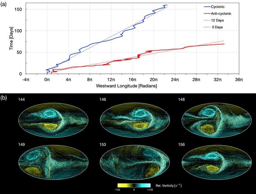
As can be seen in Fig. 5, the equilibrated flow for this setup set of motions as they evolve non-linearly. The motions, however,
is broadly characterised by three features: 1) a fast, prograde exhibit distinct life-cycles, which may be observable. One of the
(eastward flowing), zonally asymmetric equatorial jet; 2) sharp, cycles is associated with generation then decimation of modons
planetary-scale fronts which form in both the northern and southern repeating many times over 1500 planetary days of T170 simula-
hemispheres and roll up into small-scale vortices near the eastern tions.9 Qualitatively same behaviour occurs in T341 and T682 res-
terminator, particularly at the lower p-level; and, 3) planetary-scale olution simulation over shorter durations (300 planetary days). Sig-
storms that exhibit a variety of quasi-periodic stable states, as well
as transitions between those states. We stress that, when the flow
is adequately resolved, the equatorial jet is not zonally symmet- 9 Given the lack of realistic physical parameterizations, such a long du-
© yyyy RAS, MNRAS 000, 1–??
8      J. W. Skinner & J. Y-K. Cho

Figure 5. The relative vorticity (ζ) field from a T682L20 resolution simulation at t = 100 in Mollweide projection. The dissipation order, viscosity coefficient
and time-step size are p = 8, ν16 = 2.3×10−48 and ∆t = 2×10⁻⁵ , respectively. The p-levels shown, 5.0 × 10⁻³ (a) and 9.5 × 10⁻² (b), correspond to
the mid-points of the top and bottom layers of the computational domain, respectively. The flow is dominated by two highly dynamic, planetary-scale modons
– a cyclonic modon at the sub-stellar point (at centres of the frames) and a much weaker and larger anti-cyclonic modon at the night side (the sides of the
frames). The cyclonic modon straddles an undulating, zonally-asymmetric equatorial jet at both p-levels. The equatorial jet in a) is halted just to the east of
the sub-stellar point and breaking throughout its “core” (along the equator): the jet core is where there is a jump in ζ in the meridional direction (near the
equator). The equatorial jet in b), in contrast, is rolling up much more prominently at its northern and southern edges. The cyclonic modons in both frames emit
large-amplitude gravity waves and generate thousands of small-scale vortices at their peripheries; the anticyclonic modons are barely visible at both p-levels
because they are more diffused and lack sharp bounding fronts in these frames. Both cyclonic and anticyclonic modons are highly dynamic and exhibit periodic
life-cycles in which they generally (but not always) migrate westward around the planet, while strongly interacting with other flow structures – e.g. storms,
jets and waves.

nificantly, both cyclonic and anti-cyclonic modons are highly dy-                  2015; Skinner & Cho 2021). However modons were not the fo-
namic and chaotically translate westward, in general, while under-                 cus of these studies. Moreover, past studies were performed with
going frequent changes in size, shape, orientation and strength as                 lower resolution and/or stronger numerical viscosity than in the
they do so. These behaviours can easily be missed when averaged                    present study. Since capturing the fine-scale structures (and, in par-
fields or quantities are strictly used to study the atmosphere; see e.g.           ticular, their influence on the large-scale structures) is crucial, high-
discussions in Cho, Polichtchouk & Thrastarson (2015) and Cho et                   resolution and minimal over-dissipation are necessary ingredients
al. (2019). As already discussed, both hetons and modons can form                  in accurately modelling modons. Specifically, having extensively
in simulations encompassing a wide range of pressure levels. This                  investigated the influence of well-resolved fine-scale structures,
includes simulations which include the deeper region, where the                    we find the longevity, dynamism and multiple state behaviours
thermal forcing is not applied. This is shown explicitly in Fig. 6.                of planetary-scale modons are fundamentally affected. Below the
      In Fig. 6, two “deep atmosphere” simulations (i.e. those with                T170 horizontal resolution and when low-order viscosity and/or
pbot > 1) are presented. The resolution of the simulations is                      large viscosity coefficient are used, modons are markedly diffused
T170L200; and, p = 8, ν16 = 10−38 and ∆t = 8 × 10⁻⁵ . The                          and translate smoothly around the planet – if they move at all. Strict
pbot is different between the two simulations, with values of 1 and                numerical convergence does not appear to be achieved until at least
10 (left and right columns, respectively). The ζ-field is displayed                T341 resolution (Skinner & Cho 2021).
in all the frames. Fig. 6a shows the top of a hetonic quartet, which
forms in the deep atmosphere simulations at early times – as in the                      Fig. 7 presents the longitude positions of the modon centroids
“shallow atmosphere” simulation (i.e. with pbot = 0.1, presented                   from the T682L20 simulation in Fig. 5, as an illustrative example.
in Fig. 4). The meridional symmetry is strong at the time shown,                   Such plots are instructive, particularly for observations, because of
but quickly breaks shortly thereafter. Figs. 6(b–d) present modons                 the modons’ strong influence in redistributing large patches of hot
in deep atmosphere simulations at different p-levels and times. As                 and cold air across the planet – as discussed more in detail below.
can be seen, modons occur near the top of the modelled domain                      In the figure, blue and red lines show the longitudinal distance tra-
independently of the location of the domain bottom, provided a                     versed by the cyclonic and anticyclonic modons, respectively. Dot-
sufficient number of vertical levels are used to span the domain.                  ted lines indicate linear fits, with the 2π-traversal periods indicated
The modons shown here also translate around the planet and peri-                   in the legend. As already noted, the behaviours are quantitatively
odically break and reform into several different configurations of                 different at different resolution and dissipation order. However, the
vortices, similar to the behaviour in the shallow atmosphere simu-                 general behaviour here is very roughly similar down to T85 res-
lations.                                                                           olution – provided p = 8 dissipation order is employed (Skinner
      We note here that several past studies employing a similar                   & Cho 2021): in particular, the cyclonic modon’s westward trans-
setup have captured vortex dipole structures (e.g. Thrastarson &                   lation is observed, but the modon is sluggish and is devoid of the
Cho 2010; Heng et al. 2011; Cho, Polichtchouk & Thrastarson                        non-linear or oscillatory motions (which arise when small-scale ed-
                                                                                   dies are captured at T341 and above resolutions). Essentially all
                                                                                   previous extrasolar planet simulations have been performed with
ration simulation should not be taken too literally – particularly given the       less than T341 resolution and p = 8 dissipation order – especially
short τth in the upper part of the domain.                                         ones that use the current setup and are three dimensional.

                                                                                                                             © yyyy RAS, MNRAS 000, 1–??
Modons on Tidally Synchronised Extrasolar Planets                                     9

Figure 6. Two “deep atmosphere” simulations with pbot = 1 (left) and pbot = 10 (right) at different times (labeled, top). The resolution of both simulations
are T170L200; both are set up identically and carried out with p = 8, ν16 = 10−38 and ∆t = 8×10⁻⁵ . The ζ fields at the times indicated are shown in
Mollweide projection centred on the sub-stellar point, and the times are chosen when the modons are clearly in view (near the sub-stellar point); the winds
are overlaid with the reference vector length (in units of m s−1 , which is equal to 3.025×10⁻³ in Rp τ −1 units), adjusted in each frame for visual clarity.
Frame (a) shows the top of a hetonic quartet, which also forms in these deep simulations at early times (as in the “shallow atmosphere” simulations); the
flow field is not yet turbulent at this time, but sharp fronts have already developed. Frames (b–d) show coherent modons are present at various times and at
various p-levels. Post the initial transient stage, the modons evolve, embedded in turbulent fields containing many smaller scale flow structures – including
gravity waves (striations in ζ). Here modons generally migrate westward (chaotically) around the planet – periodically breaking or transitioning to different
configuration states (again, as in the shallow atmosphere simulations). Broadly, the flow tends to be more zonal and often contains an extra planetary-scale
cyclonic modon as pbot → 20, particularly in the very deep fields (b and d), compared with the flow in the shallow atmosphere simulations at this (and lower)
horizontal resolution; but, the flow becomes much less zonal and is similar to that of the shallow atmosphere simulation at a higher horizontal resolution –
particularly in the region p . 1 (Skinner & Cho 2021; Cho, Skinner & Thrastarson 2021).

     In the figure, modons are seen executing westward transla-                   riod of time (up to ∼10 planetary days).10 Near the sub-stellar
tions around the planet in the bulk, on a few to ∼20 planet-day                   point, the cyclonic modon generates and interacts with a very large
periods. But, there are pauses, reversals of direction and short pe-              number of small-scale storms of opposing signs to the cyclonic
riod (. day) oscillations superimposed on the bulk motion. This                   modon in the northern and southern hemispheres (Fig. 5b). This ef-
is due to the strong interaction with small-scale structures. Fre-                fectuates the meridional (as well as enhances the zonal) symmetry
quently, the modons break and reform at the end of their “life-                   breaking, causing the modon to oscillate about the sub-stellar point
cycles” (e.g. Fig. 8). However, while both types of modon feature                 by ∼10◦ in longitude. This is concomitant with a decrease in the
quasi-periodic life-cycles, they generally display large differences              modon’s size and strength as well as an increase in angular sepa-
in periodicity and phase between them – after the initial, formative              ration between the constituent cyclones, thus rendering the modon
period of ∼10 planetary days.                                                     susceptible to further perturbations. This is a characteristic prop-
                                                                                  erty of modons in the ageostrophic regime. After the extended pe-
      In a typical life-cycle of the cyclonic modon, the modon first
forms slightly westward of the sub-stellar point and initially trans-
lates eastward – consistent with its cyclonic character in the back-              10  In some cases, it can be as long as ∼100 planetary days initially, if the
ground of no, or very weak, motion. After reaching the sub-stellar                zonal symmetry remains unbroken or only very mildly broken (e.g. when
point, the modon often “hangs” in this position for an extended pe-               the forcing is more symmetric or dissipation steers the flow).

© yyyy RAS, MNRAS 000, 1–??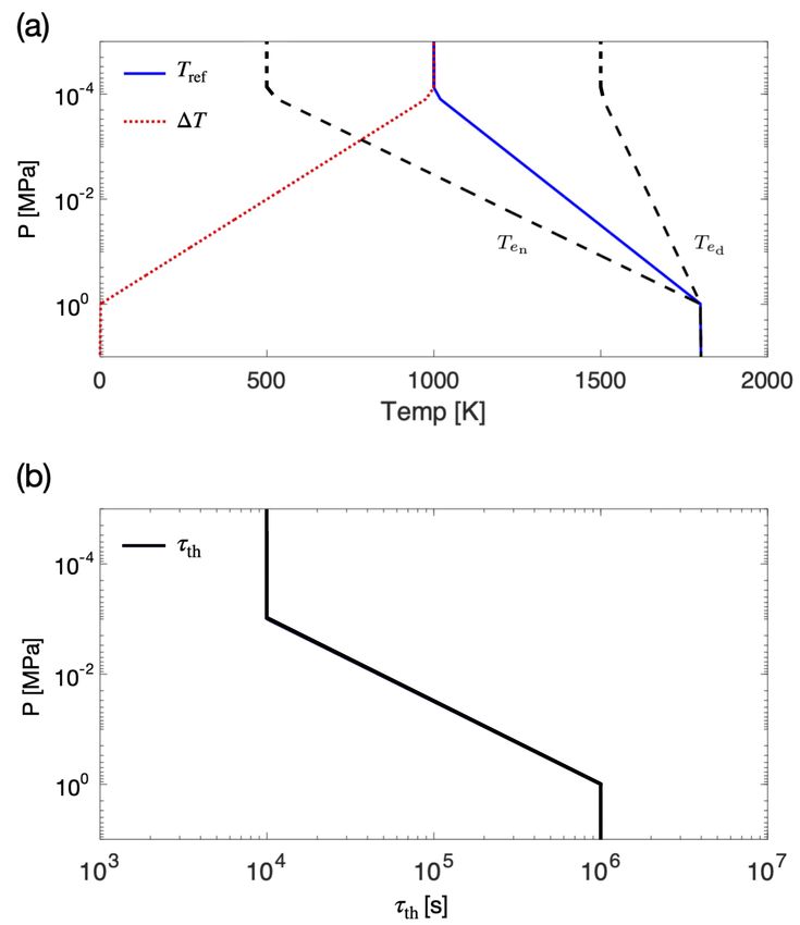
10       J. W. Skinner & J. Y-K. Cho

Figure 7. (a) Longitude position of the modon centroids (in radians) westward of the sub-stellar point, as a function of time t = [0, 125] and at p = 0.1, from
the simulation in Fig. 5. Blue and red lines correspond to the cyclonic and anticyclonic modon centroid trajectories, respectively. Dotted lines are constant
westward migration rate fits with periods 12 and 5, as indicated in the legend. Both modons exhibit quasi-periodic life-cycles in which they translate chaotically
westward around the planet in the bulk, undergoing multiple excursions about a smooth straight-line trajectory. On multiple occasions, modons pause at the
day-side (night-side) and oscillate to either side of the sub-stellar (anti-stellar) point, before continuing on. Such behaviours are significant for observations.
(b) The relative vorticity (ζ) field from the simulation shown in Fig. 5 at p ∼ 0.1 and in Mollweide projection showing a single cycle of a modon’s westward
translation around the planet.

riod near the sub-stellar point, the modon moves westward, past the                  ence of the planet near the equator. Ultimately, this is related to the
western terminator and quickly traverses the night-side to reach the                 asymmetry of the thermal forcing (recall that the night-side equi-
eastern terminator in a nearly continuous motion. The traversal usu-                 librium temperature is uniform and lower than the day-side temper-
ally takes no longer than ∼5 planetary days. Finally, at the eastern                 ature). Consequently, the variability can be considerably different,
terminator, the modon’s constituent cyclones uncouple and dissi-                     depending on the latitude being viewed. This points to the impor-
pate completely or move to high latitudes – whence the cycle ends.                   tance of knowing the planet’s obliquity (or inclination angle), when
A new cyclonic modon subsequently forms on the day-side and                          interpreting atmospheric variability. Further, note that the cyclonic
the cycle begins again. In total, the cycle lasts for ∼15 (±4) plane-                and anti-cyclonic modon tracks are roughly anti-correlated in lon-
tary days, of which the modon generally occupies the day-side for                    gitude in Fig. 7; for example, the anti-cyclonic modon forms on the
∼10 planetary days.                                                                  night-side at the same time as the cyclonic modon, which forms on
                                                                                     the day-side. Such coupled behaviour presents additional “targets”
      While the anticyclonic modon’s life-cycle is qualitatively sim-
                                                                                     for current and future observations.
ilar to that the of the cyclonic modon, it is shifted in phase (longi-
tudinal location) and has a considerably shorter migration period.
The latter is because the anti-cyclonic modon is generally located
nearer to the planet’s poles and precesses only slightly off the polar
axis at high-latitudes, rather than traversing the entire circumfer-

                                                                                                                                © yyyy RAS, MNRAS 000, 1–??
Modons on Tidally Synchronised Extrasolar Planets 11
Figure 8. The ζ field, with overlaid winds (reference vector length is 1000 m s−1 , equal to 3.025 in Rp τ −1 units) at p = 0.1 from a T341L20 simulation,
with p = 8, ν16 = 1.5 × 10−43 , ∆t = 4×10⁻⁵ and vertical range of [0, 0.1]. The four frames illustrate the onset of a secondary equilibrium state that arises
in the simulations. In this sequence, a modon breaks apart into fast moving, uncoupled cyclones; and, the atmosphere is rapidly mixed as a consequence. At
t = 40 a cyclonic modon, which has spent an extended period of time positioned at the sub-stellar point, migrates eastward towards the night-side rather than
continuing on its usual westward direction (a). As the modon reaches the eastern terminator (t = 53), it encounters fast flow from the night-side and shears
apart, inducing very high amplitude undulations of the equatorial jet (b). At t = 55, both the equatorial jet and the cyclonic modon are converted into small-
scale storms, which are transported westward around the planet by very high-amplitude Rossby waves (c). At t = 56, the small-scale storms coalesce into
large-scale cyclones and the polar vortices break up (d). The atmosphere undergoes a period of vigorous mixing before a new modon forms on the day-side.
This sequence of patterns recurs quasi-periodically over the duration of the simulation.
The above discussion suggests a multitude of quasi- ing patterns” – a “diffluent block” and an “omega block”.12 In the
equilibrium flow states 11 . These states are associated with distinct figure, blocking actions rapidly mix and chaotically churn the at-
flow configurations and periodicities and lasts for extended periods mosphere over a several-day time-scale. The transition is from the
of varying durations. Moreover, multiple transitions between the diffluent block to an omega block and eventually back to the difflu-
states within a single simulation occur as well. In general, the set ent block (often after a complete dispersal of the original modon,
of available states vary with p-levels; but, they are often correlated. as shown). We note that the modon in this example had previously
The overall behaviour is generic across small variations in thermal completed many traversals of the planet prior to this breakup. In-
forcing profile and initial flow condition. However, as expected, the stead of continuing its westward translation, this modon translates
behaviours is quantitatively different at lower resolution and even eastward across the sub-stellar point close to the eastern terminator
qualitatively different below T85 resolution. The latter is because (Fig. 8a), where it starts to tilt in the counter-clockwise direction
simulations below the T85 resolution (particularly with p < 8) pro- (Fig. 8b). In the latter, the shearing modon disrupts the equatorial
duce modons (when they are able) that are not dynamic (Skinner & jet, generating many hundreds of small-scale storms in the process.
Cho 2021). After one to two planetary days, the modon is nearly sideways,
Fig. 8 presents an example of a state transition that frequently fully into the omega state (Fig. 8c). At this point, the small-scale
occurs in the current setup. The four frames in the figure illustrate storms generated are carried westward from the night-side to the
the key stages of a transition between two states known as “block-
12 In meteorology, blocks are large-scale weather patterns that are nearly
11 We define “quasi-equilibrium” as a state that persists over a long dura- stationary and effectively block and redirect flows (Rex 1950; Woolings et
tion – i.e. over a period much longer than max{τth , τad }, when τth < ∞. al. 2018).
© yyyy RAS, MNRAS 000, 1–??You can also read