Mesospheric gravity wave activity estimated via airglow imagery, multistatic meteor radar, and SABER data taken during the SIMONe-2018 campaign
←
→
Page content transcription
If your browser does not render page correctly, please read the page content below

Atmos. Chem. Phys., 21, 13631–13654, 2021
https://doi.org/10.5194/acp-21-13631-2021
© Author(s) 2021. This work is distributed under
the Creative Commons Attribution 4.0 License.

Mesospheric gravity wave activity estimated via airglow imagery,
multistatic meteor radar, and SABER data taken during the
SIMONe–2018 campaign
Fabio Vargas1 , Jorge L. Chau2 , Harikrishnan Charuvil Asokan2,3 , and Michael Gerding2
1 Department  of Electrical and Computer Engineering, University of Illinois at Urbana-Champaign, Urbana, IL 61801, USA
2 LeibnizInstitute of Atmospheric Physics and the University of Rostock, 18225 Kühlungsborn, Germany
3 Laboratoire de Mécanique des Fluides et d’Acoustique, CNRS, École Centrale de Lyon,

Université Claude Bernard Lyon 1, INSA de Lyon, Écully, France

Correspondence: Fabio Vargas (fvargas@illinois.edu)

Received: 27 August 2020 – Discussion started: 8 September 2020
Revised: 28 June 2021 – Accepted: 5 August 2021 – Published: 13 September 2021

Abstract. We describe in this study the analysis of small and   (11 % of the events) transport 50 % of the total measured
large horizontal-scale gravity waves from datasets composed     FM . Likewise, wave events of FM > 10 m2 s−2 (2 % of the
of images from multiple mesospheric airglow emissions as        events) transport 20 % of the total. The examination of large-
well as multistatic specular meteor radar (MSMR) winds col-     scale waves (λh > 725 km) seen simultaneously in airglow
lected in early November 2018, during the SIMONe–2018           keograms and MSMR winds revealed amplitudes > 35 %,
(Spread-spectrum Interferometric Multi-static meteor radar      which translates into FM = 21.2–29.6 m2 s−2 . In terms of
Observing Network) campaign. These ground-based mea-            gravity-wave–mean-flow interactions, these large FM waves
surements are supported by temperature and neutral density      could cause decelerations of FD = 22–41 m s−1 d−1 (small-
profiles from TIMED/SABER (Thermosphere, Ionosphere,            scale waves) and FD = 38–43 m s−1 d−1 (large-scale waves)
Mesosphere Energetics and Dynamics/Sounding of the At-          if breaking or dissipating within short distances in the meso-
mosphere using Broadband Emission Radiometry) satellite         sphere and lower thermosphere region.
in orbits near Kühlungsborn, northern Germany (54.1◦ N,
11.8◦ E). The scientific goals here include the characteriza-
tion of gravity waves and their interaction with the mean
flow in the mesosphere and lower thermosphere and their
relationship to dynamical conditions in the lower and up-       1   Introduction
per atmosphere. We have obtained intrinsic parameters of
small- and large-scale gravity waves and characterized their    Atmospheric gravity waves represent a class of atmosphere
impact in the mesosphere via momentum flux (FM ) and mo-        oscillations where buoyancy is the restoring force. These
mentum flux divergence (FD ) estimations. We have veri-         waves transport momentum and energy over large distances
fied that a small percentage of the detected wave events        within the atmosphere and have as primary sources tropo-
is responsible for most of FM measured during the cam-          sphere disturbances like flow over topography, convective
paign from oscillations seen in the airglow brightness and      systems, or jets (e.g., Vincent and Alexander, 2020). To pre-
MSMR winds taken over 45 h during four nights of clear-         serve kinetic energy, the amplitudes of the gravity waves
sky observations. From the analysis of small-scale gravity      grow nearly exponentially as they propagate upward into less
waves (λh < 725 km) seen in airglow images, we have found       dense air at higher altitudes. When these waves break and
FM ranging from 0.04–24.74 m2 s−2 (1.62 ± 2.70 m2 s−2 on        dissipate, they deposit their momentum and energy into the
average). However, small-scale waves with FM > 3 m2 s−2         background atmosphere. This affects the atmosphere over a
                                                                broad range of scales, from local generation of turbulence

Published by Copernicus Publications on behalf of the European Geosciences Union.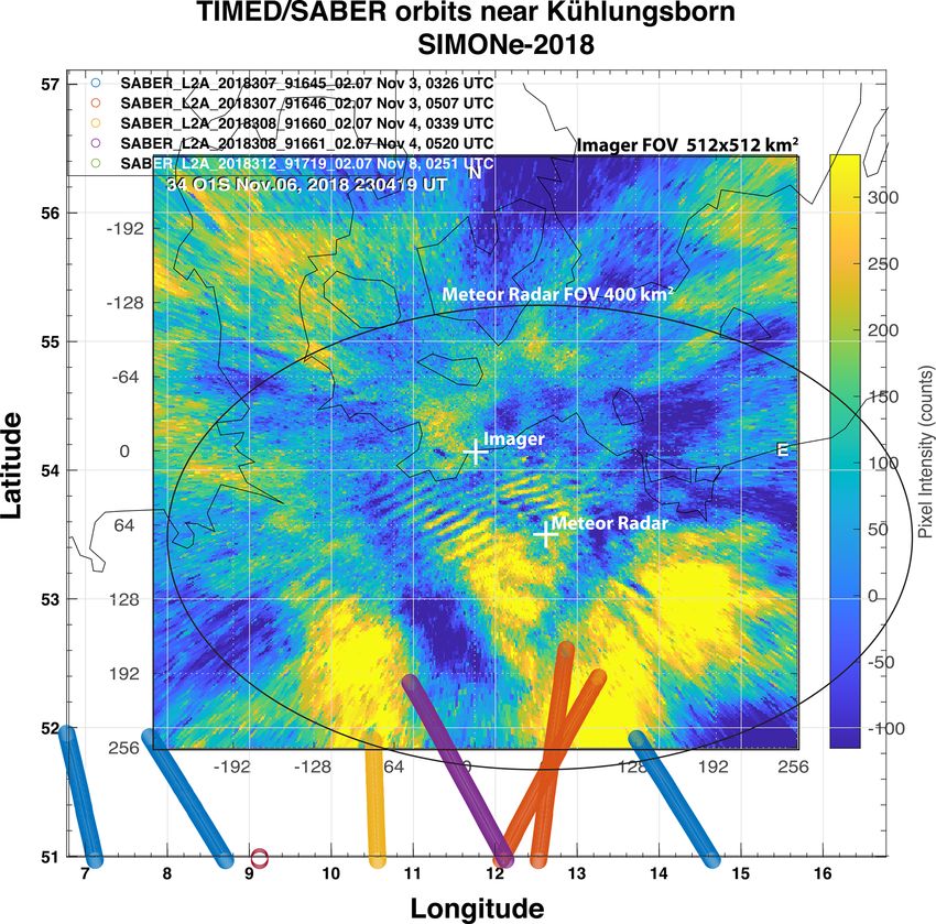
13632                                            F. Vargas et al.: Gravity wave activity during the SIMONe–2018 campaign

to forcing of large-scale circulation (Fritts and Alexander,          To bridge gaps in gravity wave dynamics while estimating
2003; Vincent and Alexander, 2020).                                their FM , an observation campaign named SIMONe–2018
   This dynamical forcing is most prominent within the             (Spread-spectrum Interferometric Multi-static meteor radar
mesosphere and lower thermosphere (MLT) at altitudes of            Observing Network) was carried from 2–9 November 2018,
typically 50–130 km. Within this range, a large fraction of        to collect a large number of specular meteor echoes from
upward-propagating gravity waves reach their maximum am-           several locations (e.g., Vierinen et al., 2019; Charuvil et al.,
plitudes and break. The resulting dynamical forcing causes a       2020). Also, an all-sky airglow imager system running out of
global-scale circulation within the mesosphere with strong         the Leibniz Institute of Atmospheric Physics, Kühlungsborn,
upwelling within the summer polar region and downwelling           Germany, observed the region in parallel to provide image
within the winter polar region (Houghton, 1978; Holton,            data of the mesosphere and the horizontal structure of atmo-
1984). Adiabatic cooling and heating connected to this cir-        spheric oscillations during the campaign.
culation cause thermal conditions within the mesosphere to            SIMONe–2018 campaign measurements permit us to
deviate greatly from radiative equilibrium (Solomon et al.,        study distinct spatial and temporal scales of gravity waves
1987; Vargas et al., 2015).                                        perturbing the background wind and the airglow simulta-
   The role of gravity waves is further complicated as they        neously. In this paper, we have analyzed all-sky imager
interact with the background flow as they propagate through        (ASI) airglow images and multistatic specular meteor radar
the atmosphere. This results in an altitude-dependent filter-      (MSMR) wind data to access small-scale as well as large-
ing of the gravity wave spectrum by the background wind,           scale gravity wave dynamics using two different analysis
planetary, and tidal waves. The gravity wave spectrum reach-       methods for each wave category. Airglow images are pro-
ing higher altitudes thus carries an imprint of the dynamics       cessed directly using our auto-detection method for small-
at lower altitudes. Interactions between gravity waves and         scale (< 725 km), short-period (< 1 h) gravity waves aided
the mean flow and subsequent wave breaking then gener-             by MSMR background wind measurements for Doppler cor-
ate secondary waves within the mesosphere that propagate           rection of wave-apparent periods (τo ). For nights present-
both upward and downward. This happens through the cre-            ing obvious large-scale (> 725 km), long-period (> 1 h) os-
ation of temporally and spatially localized momentum and           cillations, wave features are studied via direct examination
energy fluxes, which successively create strong local body         of large-amplitude wind fluctuations and airglow keogram
forces and flow imbalances which then excite the secondary         spectral analysis. We have also obtained measurements of
waves (Fritts et al., 2006; Vargas et al., 2016; Vadas et al.,     the neutral density, temperature, and OH emission volume
2018; Vadas and Becker, 2018; Becker and Vadas, 2018).             emission rates from the SABER instrument (Russell et al.,
   While today the essential nature of the wave-driven circu-      1999; Mlynczak, 1997) aboard the NASA TIMED (Thermo-
lation of the middle atmosphere is known, important mecha-         sphere, Ionosphere, Mesosphere Energetics and Dynamics)
nisms and interactions remain to be quantified. Most notably,      satellite (http://saber.gats-inc.com, last access: 6 September
this concerns wave sources, wave dissipation, and therefore        2021) to determine the state of the mesosphere region near
the resulting forcing of the mean flow. A decisive quan-           the observatory during the campaign. This study shows re-
tity to be specified is the directional FM , including its alti-   markable instances of waves perturbing the airglow and the
tude dependence and its spectral distribution with reference       wind, providing a singular opportunity to examine the linear
to horizontal (λh ) and vertical (λz ) wavelengths. Ern et al.     gravity wave theory’s predictions and the occurrence of grav-
(2011) have provided global distributions of gravity wave          ity waves perturbing multiple mesospheric quantities simul-
FM in the mesosphere for the first time using global temper-       taneously. The main contributions here regard the fraction of
ature measurements by the Sounding of the Atmosphere us-           observed waves carrying substantial FM with the potential to
ing Broadband Emission Radiometry (SABER). They have               impart significant changes in the 75–110 km dynamics since
shown clearly the dependency of gravity wave FM deposi-            we show evidence that most observed waves likely experi-
tion according to latitude and longitude (non-uniform longi-       ence dissipation in that region.
tudinal distribution of flux) at different altitude levels from
the stratosphere up to the mesosphere along with their sea-
sonal and longer-term variations. Also, attempts of estimat-       2     Instrumentation and data
ing FM of small-scale, short-period waves using multiple ob-
servation platforms such as aircraft, lidar, airglow sounders,     2.1    All-sky airglow imager
radars, and satellites have been done (e.g, Suzuki et al.,
2010; Bossert et al., 2015), while Gong et al. (2019) and          An all-sky imager (ASI) assembled at Boston University
Reichert et al. (2019) have relied on lidar, meteor radar, and     was deployed in late 2016 at the Leibniz Institute of At-
SABER data to study large-scale, long-period waves perturb-        mospheric Physics (IAP) in Kühlungsborn, Germany. The
ing the mesosphere temperature and the winds simultane-            imager is equipped with an Andor back-illuminated bare
ously. These studies report attempts to characterize the wave      CCD camera and a 30 mm fish-eye lens which record sev-
field and provide FM estimations of observed events as well.       eral nightglow emissions over the entire 180◦ of the night

Atmos. Chem. Phys., 21, 13631–13654, 2021                                          https://doi.org/10.5194/acp-21-13631-2021
F. Vargas et al.: Gravity wave activity during the SIMONe–2018 campaign                                                         13633

Table 1. Configuration of the all-sky imager system used to collect     associated with large-scale, long λh gravity waves perturb-
airglow images during the SIMONe–2018 campaign. Airglow im-             ing the green line layer. For instance, note in the meridional
ages of the campaign are available at http://sirius.bu.edu/data/. NaD   keogram of 3–4 November the orientation of the brightness
represents a sodium atom at the D transition line.                      variation associated with a large-scale wave in a region tilted
                                                                        from top to bottom during 19:30 to 22:30 UTC, indicating a
    Filter     Emission              Wavelength      Integration        coherent oscillation traveling from north to south. The tilt in
                                           (nm)         Time (s)        the brightness region is not pronounced in the zonal keogram
    RG695      OH                  695.0–1050.0              15         for the same time span, indicating a small, negligible wave
    6050C      Background OH              605.0             120         component in the west–east direction. Perturbations of the
    5893C      NaD                        589.3             120         same nature are also seen in the O2 and OH emissions for the
    8660C      O2 (0,1)                   864.5             120         same nights.
    5577C      O(1 S)                     557.7             120             The right-hand side panels of Fig. 1 show zonal and merid-
    6300C      O(1 D)                     630.0             120         ional keograms built using time–difference (TD) airglow im-
                                                                        ages. Time–difference operation involves subtracting an im-
                                                                        age from the previous one (same emission) with the goal of
sky. Andor’s iKon-M 934 camera is a 1024 × 1024 array                   filtering out long-term variations in the airglow brightness
and 13 µm pixel pitch with a 13.3 × 13.3 mm active image                (e.g., Swenson and Mende, 1994; Swenson and Espy, 1995;
area. High sensitivity is achieved through a combination                Tang et al., 2005; Vargas, 2019). The result is an image where
of > 90 % QE (quantum efficiency; back-illuminated sen-                 the contrast of shorter-period, smaller-scale oscillations is
sor), low noise readout electronics, and deep TE (thermo-               enhanced. These small-scale waves show up in the keograms
electric) cooling down to −60◦ C. The ASI system uses six               as tilted bright/dark bands. Because long-period waves are
interference filters enabling the observation of four meso-             suppressed, time–difference keograms permit rapid access to
sphere airglow emissions with a background filter for the               the activity of short-period waves each night.
hydroxyl emission. A filter for the thermospheric redline (at
630.0 nm) is also available, but images of this emission were           2.2   Multistatic specular meteor radar
not taken during SIMONe–2018 due to filter technical is-
sues. The imaging system operates autonomously via a PC                 During the SIMONe–2018 campaign, MSMR measurements
on a nightly basis during moonless periods. Images are ob-              were obtained continuously for 7 d. Briefly, the campaign
tained on a continuously repeating cycle every ∼ 2 min with             consisted of 14 multistatic links that were obtained by us-
each particular filter accessed every ∼ 10 min. The specifi-            ing two pulse transmitters located in Juliusruh (54.63◦ N,
cations of filter wavelengths and integration times are in Ta-          13.37◦ E) and Collm (51.31◦ N, 13.00◦ E), respectively, and
ble 1. Emission altitudes are discussed in Sect. 2.3. Prepro-           one coded–continuous wave transmitter located in Kühlungs-
cessed, low-resolution images collected by the ASI are avail-           born. Eight receiving sites were used to receive the scattered
able for visualization at http://sirius.bu.edu/data/ (last access:      signal of at least one transmitter. This campaign combines the
6 September 2021). Raw images used in this study are avail-             multistatic approach called MMARIA (Multistatic Multifre-
able at https://doi.org/10.13012/B2IDB-8585682_V1 (Var-                 quency Agile Radar Investigations of the Atmosphere) (Sto-
gas, 2021).                                                             ber and Chau, 2015) with the SIMONe (Spread Spectrum In-
   The SIMONe–2018 campaign was carried out for more                    terferometric Multistatic meteor radar Observing Network)
than a week, but clear skies were seen only during four                 concept (Chau et al., 2019). In the latter case a combina-
nights, which limited the optical observations with the all-            tion of spread-spectrum, multiple-input–multiple-output, and
sky imager. The sky conditions for the four clear nights are            compressing sensing radar techniques is implemented (Vier-
summarized in Fig. 1 by zonal and meridional keograms                   inen et al., 2016; Urco et al., 2018, 2019). The winds used
of the O(1 S) emission. Appendix C discusses in detail how              in this work have been obtained with a gradient method, i.e.,
keograms are built from airglow images. The reader is also              besides the mean horizontal and vertical winds, the gradients
referred to Vargas et al. (2020) for more keogram analysis              of the horizontal components have also been obtained (Chau
information. Although only keograms of the O(1 S) emission              et al., 2017). Data from 1 d of this campaign have been used
are shown here, we have also built keograms for the other               to test a second-order statistics approach by Vierinen et al.
three mesospheric emissions, which are available as Supple-             (2019). More details of the SIMONe–2018 campaign as well
ment files of this paper.                                               as results of second-order statistics can be found in Charuvil
   The left-hand side panels of Fig. 1 show keograms built              et al. (2020).
directly from O(1 S) preprocessed images (Appendix A). The                 Here, we have used the MSMR winds in combination with
contrast of the images was optimized to show variable fea-              the airglow data to give a full characterization of the grav-
tures in the brightness present throughout the night. Long-             ity wave dynamics observed during the campaign. Figure 2
period oscillations seen in the airglow brightness on 3–4 and           shows the (a) zonal and (b) meridional background winds
6–7 November keograms indicated by the red ellipses are                 in the range of 75–105 km measured during SIMONe–2018.

https://doi.org/10.5194/acp-21-13631-2021                                             Atmos. Chem. Phys., 21, 13631–13654, 2021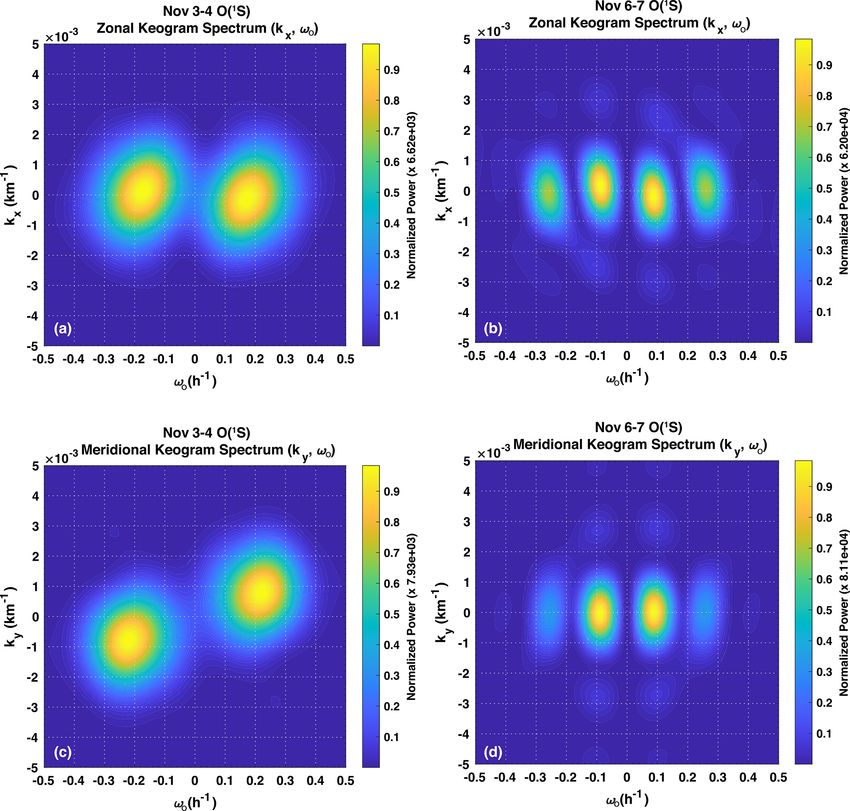
13634                                               F. Vargas et al.: Gravity wave activity during the SIMONe–2018 campaign

Figure 1. Composite keograms of O(1 S) airglow images taken on clear nights during the SIMONe–2018 campaign. The keograms in
panels (a), (c), (e), and (g) were built using light frame images, while keograms in panels (b), (d), (f), and (h) were built using TD images.
Time–difference keograms show short-period waves at higher contrast, while light frame keograms show mainly long-period oscillations.
Note the enhanced airglow brightness (red ellipses) on 3–4 November (meridional keogram) and 6–7 November (zonal keogram) associated
with large-scale gravity waves also seen in wind fluctuations of Fig. 2.

Atmos. Chem. Phys., 21, 13631–13654, 2021                                                  https://doi.org/10.5194/acp-21-13631-2021
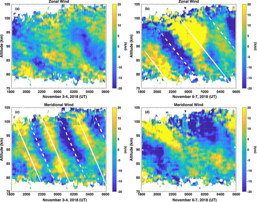
F. Vargas et al.: Gravity wave activity during the SIMONe–2018 campaign                                                              13635

Figure 2. (a) Zonal and (b) meridional wind measurements for the duration of the SIMONe–2018 campaign generated by the MSMR
network. Note the dominance of the semidiurnal tide on the horizontal wind. (c) Zonal and (d) meridional wind fluctuations of τo ≤ 4 h. Note
the presence of coherent gravity wave features (red ellipses) on 3–4 November in the meridional wind fluctuations and on 6–7 November
in the zonal wind fluctuations coincident with enhanced keogram brightness for the same nights in Fig. 1. Dashed boxes indicate hours of
simultaneous operation of the ASI and MSMR systems.

https://doi.org/10.5194/acp-21-13631-2021                                               Atmos. Chem. Phys., 21, 13631–13654, 2021
13636 F. Vargas et al.: Gravity wave activity during the SIMONe–2018 campaign
Dashed boxes indicate hours of simultaneous operation of (dT /dz = 1.6 K km−1 ) below and above the 88–99 km range.
the ASI and MSMR systems. The background wind field is Even though the satellite orbits registered during SIMONe–
calculated from the MSMR measurements using 30 min tem- 2018 were not exactly over the observatory, the instrument
poral and 1 km spatial windows. Observe the daily cycle for measurements are performed in the vertical limb plane that
z < 80 km and z > 100 km in the plots that is associated with is near or within the field of view of the imager (Fig. 3). Note
the variation in meteor detections throughout the day; the me- that the colored dots indicate where the measurements were
teor density is larger in earlier morning hours and smaller in made, not the satellite position. Thus, there is a good chance
afternoon hours. Because wind calculation relies on the num- the background atmosphere above the observation site is sim-
ber of meteors to make quality wind estimations, when not ilar to that indicated by SABER (Fig. 4), although the tem-
enough meteors are detected, the wind cannot be estimated perature might still be influenced by gravity waves once we
within a reasonable uncertainty level. The background wind have averaged only a few profiles. Because of that, we are
is dominated by a 12 h tidal oscillation presenting amplitudes confident using SABER background profiles to make infer-
larger than 50 m s−1 , but spectral analysis reveals the pres- ences about the propagation conditions for the waves seen
ence of higher tidal harmonics of 8 and 6 h (see Figs. 6 and over the observatory.
7). Figure 4d corresponds to our estimation of volume emis-
Figure 2c and d also present the zonal and meridional wind sion rate (VER) profiles for the OH, O2 , and O(1 S) airglow
fluctuations associated with oscillations caused by gravity emissions. These VER profiles were calculated using the
waves. To obtain the wind fluctuations, we first average the mean temperature, atomic oxygen, molecular oxygen, and
MSMR raw data over a 400 km2 field of view using a square molecular nitrogen profiles in Fig. 4a–b along with the re-
4 h temporal, 4 km vertical window. Then, we subtract the re- action rates of each emission from Vargas et al. (2007). The
sult from the background wind field. Note that oscillations of characteristics of each layer (measured and calculated VERs)
τo > 4 h and λz < 4 km will be suppressed but not completely are obtained from a Gaussian model (thin lines in Fig. 4d) to
eliminated in the resulting wind fluctuations. The fluctuation fit each profile from which we obtain the layer peak, width,
winds show short-period gravity waves perturbing the wind and the full width at half maximum (FWHM). The mean
that are also seen in the airglow. For instance, the oscillation characteristics of the airglow layers are presented in Table 2.
evident in the airglow brightness variation (red ellipse) for The goodness of fitting scores R 2 > 0.95 for all five VER
3–4 November (Fig. 1c, meridional keogram) is also evident curves. The layer centroids, estimated from
as coherent oscillations in meridional wind fluctuations (red R
z VER dz
ellipse) on 3–4 November (Fig. 2d). zc = R , (1)
VER dz
2.3 Satellite data (TIMED-SABER) are in general a few kilometers above the estimated layer
peaks because of departures of the actual VER vertical struc-
We have also collected observations of the SABER in- ture from the Gaussian fitting model. We have simulated the
strument on board the TIMED satellite (Russell et al., VER profile for the OH(8,3) using the SABER mean tem-
1999; Mlynczak, 1997) within 4◦ of the observation site perature and atomic oxygen profiles for the campaign. The
(Fig. 3). The profiles cover the height range from approxi- difference between the simulated OH VER and SABER OH
mately 10 km to more than 100 km. The vertical resolution is VER lies on the averages used as inputs in the VER simula-
∼ 2 km. The instrument covers ∼ 52◦ latitude in one hemi- tion. However, SABER OH VER and simulated OH VER are
sphere to 83◦ in the other in a given day. The viewing geom- much closer in structure if we use individual SABER temper-
etry alternates every 60 d due to 180◦ yaw maneuvers of the ature and oxygen profiles.
TIMED satellite (Russell et al., 1999). Approximately 1200
temperature profiles are taken each day. SABER publica-
tions are available at http://saber.gats-inc.com/publications. 3 Data analysis and results
php (last access: 6 September 2021).
A full characterization of the gravity wave field requires
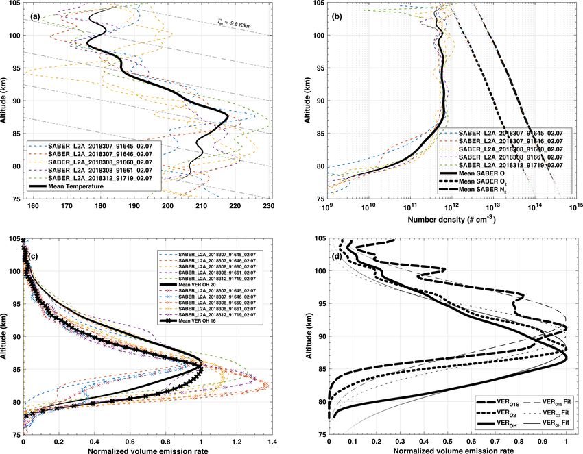
SABER profiles used here are presented in Fig. 4a–c,
knowledge of the background wind over the observation site.
while Fig. 4d shows the calculated volume emission rate of
The significant background wind acting in the vicinity of an
the mesosphere airglow emissions as explained below. The
airglow layer is a function of the vertical structure of the
thick lines in Fig. 4 indicate the mean of corresponding in-
emission (the VER) that has finite thickness (see Fig. 4d).
dividual profiles (dotted lines) for the various orbits of the
We take that into account by calculating the weighted back-
satellite during the campaign. The corresponding orbits are
ground wind (Fig. 6a–c) by using the VER of each layer
specified in the legend of each chart.
as weighting functions. The weighted wind expression for
From Fig. 4a, we can verify that the atmosphere is, on av-
a given VER is
erage, stable in the altitude range of 88–99 km since the at- R
mosphere lapse rate (dT /dz = −3.7 K km−1 ) is larger than (u, v) VER dz
(uw , vw ) = , (2)
the adiabatic lapse rate (0 = −9.8 K km−1 ) and is positive
R
VER dz
Atmos. Chem. Phys., 21, 13631–13654, 2021 https://doi.org/10.5194/acp-21-13631-2021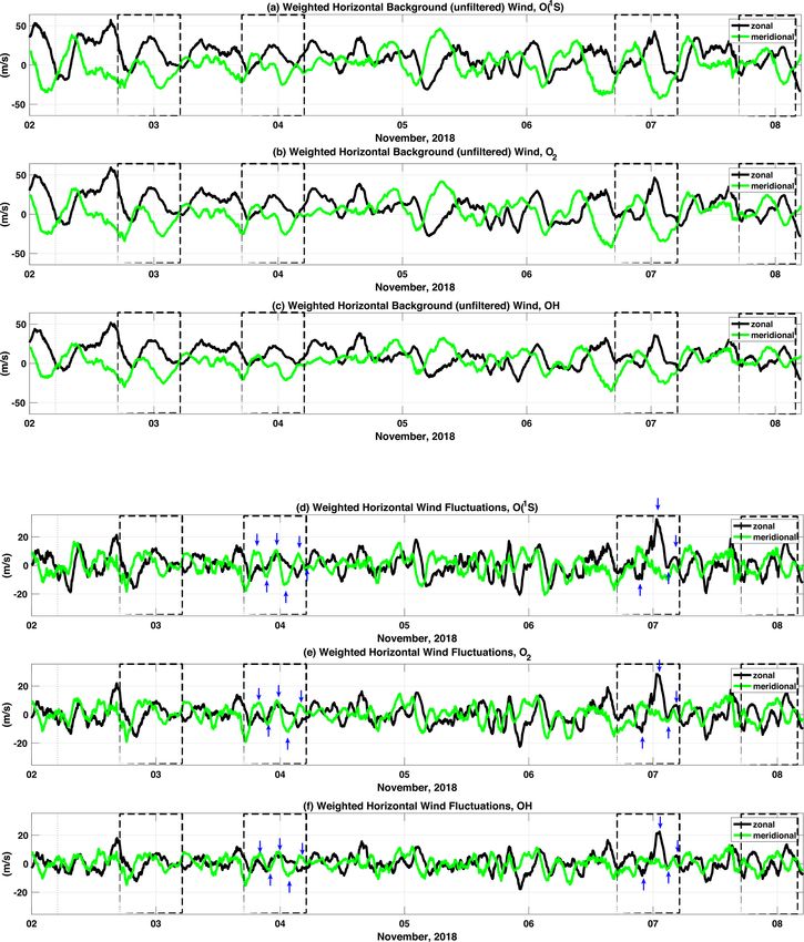
F. Vargas et al.: Gravity wave activity during the SIMONe–2018 campaign                                                               13637

Figure 3. Individual TIMED/SABER satellite orbits near Kühlungsborn during the SIMONe–2018 campaign. The colored lines represent
the location where vertical atmospheric profiles were measured, not the actual satellite locus. The day and time of each orbit is indicated in
the legend. The field of view of 512 × 512 km2 of the airglow camera projected at ∼ 95 km is indicated by the O(1 S), TD image mapped
onto geographic coordinates, while the ellipse indicates the field of view of the MSMR system. The white crosses indicates the coordinates
of the imager system in the Kühlungsborn observatory and the meteor radar system.

Table 2. Centroid, peak, and FWHM of the OH, O2 , and O(1 S) layers measured and calculated using TIMED/SABER data collected near
Kühlungsborn during the SIMONe–2018 campaign.

                             Emission     Wavelength     Origin        Layer centroid    Layer peak     FWHM
                                                                                (km)           (km)       (km)
                             OH(A)        2.1 µm         SABER                 ∼ 87.3         ∼ 86.4     ∼ 14.3
                             OH(B)        1.6 µm         SABER                 ∼ 85.8         ∼ 84.8     ∼ 12.5
                             OH(8,3)      727.3 nm       simulation            ∼ 89.4         ∼ 86.5     ∼ 18.7
                             O2 (0-1)     864.5 nm       simulation            ∼ 91.1         ∼ 88.0     ∼ 14.6
                             O(1 S)       557.7 nm       simulation            ∼ 93.3         ∼ 91.4     ∼ 16.7

where uw and vw are the weighted zonal and meridional                    agonal across the field of view of an airglow image mapped
winds (Fig. 6), respectively.                                            onto a 512 × 512 km2 grid. Thus, a 725 km horizontal-scale
                                                                         wave would present one crest and one trough fitting the im-
3.1   Short-scale gravity wave analysis                                  age frame entirely. More details about raw airglow image
                                                                         preprocessing can be found in Appendix A.
We have defined here as small-scale the waves presenting                    The majority of waves observed during SIMONe–2018
λh < 725 km, while large-scale waves present λh > 725 km.                are small-scale, fast oscillations of τi < 1 h. The keograms
This 725 km threshold corresponds to the length of the di-

https://doi.org/10.5194/acp-21-13631-2021                                                Atmos. Chem. Phys., 21, 13631–13654, 2021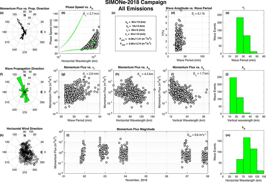
13638                                                 F. Vargas et al.: Gravity wave activity during the SIMONe–2018 campaign

Figure 4. (a) Temperature, (b) atomic oxygen, molecular oxygen, molecular nitrogen number densities, and (c) OH20 (2.1 µm OH(A)) and
OH16 (1.6 µm OH(B)) volume emission rates collected by TIMED/SABER satellite near Kühlungsborn during the SIMONe–2018 campaign
within 4◦ of latitude or longitude of the observatory. (d) Calculated volume emission rates for OH(8,3), O2 (0,1), and O(1 S) layers (thick
black lines) using SABER mean profiles in panels (a) and (b). Colored dotted lines in (a), (b), and (c) indicate individual orbits of the satellite,
while thick lines indicate the mean of the individual orbits. Gray dash–dot lines in (a) indicate the adiabatic lapse rate 0ad = −9.8 K km−1 .
Thinner black lines in (d) are Gaussian fits of the calculated VER profiles. Individual VER airglow layer features for both measured and
calculated VER are in Table 2. We have used SABER data version 2.07 to compose these plots.

of Fig. 1 (right-hand side panels) show the most promi-                     waves as seen in the original images. Further details about
nent waves of this category registered during the clear nights              this correction and the auto-detection method are found in
of the campaign. These short-scale gravity waves are an-                    Appendix B.
alyzed here using the auto-detection method (Tang et al.,                      Figure 5 shows the results from the auto-detection
2005; Vargas et al., 2009; Vargas, 2019). The auto-detection                method for all the emissions recorded during SIMONe–
method relies on three sequential airglow frames to obtain                  2018. Weighted background winds in Fig. 6a–c were used to
two time–difference images used in the cross-spectral anal-                 carry out the Doppler shift correction on τo . Thus, the param-
ysis to obtain gravity wave parameters. The calculation of                  eters shown correspond to intrinsic properties of the waves.
time–difference images leads to a change in the amplitude of                We have calculated the error bars for the parameters of each
the waves (in the TD images compared to the original ones).                 wave event measured using the methodology in Vargas et al.
The amplitude influences the Fourier analysis and therefore                 (2019). The average error of each parameter is shown in their
also the result of the cross-correlation. However, this issue               respective charts in Fig. 5. Since we rely on a set of three
is properly taken care of by restoring the amplitude of the                 images at the time to compute the cross-spectrogram of a

Atmos. Chem. Phys., 21, 13631–13654, 2021                                                      https://doi.org/10.5194/acp-21-13631-2021
F. Vargas et al.: Gravity wave activity during the SIMONe–2018 campaign                                                               13639

Figure 5. Short-period wave parameters obtained from OH, O2 , O(1 S), and Na airglow image analysis using the auto-detection method
(Tang et al., 2005; Vargas et al., 2009; Vargas, 2019). The mean measurement error is indicated in the chart of each wave parameter. Plots of
waves detected in each emission separately are in the Supplement of this paper.

set, the time span of each set is about 20 min. It is possible           75–125 km. Waves transporting large FM are mainly oriented
that the observed wave events represent waves independent                towards the northwest and southwest (Fig. 5a), but the polar
from one another because the observed waves have relatively              histogram in Fig. 5f shows a large number of waves traveling
long vertical wavelength and propagate vertically fast under             southeastward into the dominant wind orientation (Fig. 5k).
weak horizontal winds. However, we recognize that this is                Estimated τi shown in Fig. 5e ranges within 20–40 min, with
not always the case, and, as the oscillations slow down as               intrinsic phase speeds in the interval of 30–100 m s−1 during
they propagate vertically, their residence time within a given           the campaign (Fig. 5b). The largest wave relative amplitude
airglow layer could be long. Therefore, some of the detected             estimated from the images is 7 % in Fig. 5d, but this does not
waves could have been counted twice while evaluating the                 necessarily translate into large FM waves, which depends on
average momentum flux and other wave statistics.                         other wave parameters.
   Because every image of a given airglow layer is taken                    Since the auto-detection method returns wave intrinsic pa-
at 10 min pace (the filter wheel cycle period), we are only              rameters, we are able to estimate FM of every measured event
able to resolve wave-apparent periods > 20 min. On the other             (e.g., Vargas et al., 2007). Figure 5l shows the daily FM of
hand, the exposure time used here is mostly 2 min; aliasing              waves detected during SIMONe–2018, with larger FM waves
could be present due to this relatively long exposure time.              appearing on 2–3 and 3–4 November. The momentum flux
However, we have assured the aliasing is minimal in this case            vs. intrinsic wave period chart (Fig. 5g) reveals a tendency
because there is no smudging of the small-scale wave struc-              of larger τi waves carrying larger FM . Conversely, Fig. 5h
tures seen in the images.                                                (Fig. 5i) reveals that large λh (λz ) waves associate with small
   The top-center box (Fig. 5c) contains a statistics summary            FM quantities.
of the measured wave parameters. Figure 5j shows λz rang-
ing from 10 to 40 km, while λh in Fig. 5m clusters around

https://doi.org/10.5194/acp-21-13631-2021                                               Atmos. Chem. Phys., 21, 13631–13654, 2021
13640                                              F. Vargas et al.: Gravity wave activity during the SIMONe–2018 campaign

Figure 6. (a) O(1 S), (b) O2 , and (c) OH volume emission rate weighted zonal and meridional background (unfiltered) winds. (d) O(1 S),
(e) O2 , and (f) OH volume emission rate weighted zonal and meridional wind fluctuations. Wind fluctuations were obtained first by averaging
the wind over 400 km2 field of view using a 4 h temporal, 4 km vertical window to obtain winds representing large-scales variations and then
subtracting these estimates from the background wind field. The vertical blue arrows indicate coherent wind fluctuations also seen in the
airglow brightness. Dashed boxes indicate hours of simultaneous operation of the ASI and MSMR system.

Atmos. Chem. Phys., 21, 13631–13654, 2021                                                 https://doi.org/10.5194/acp-21-13631-2021
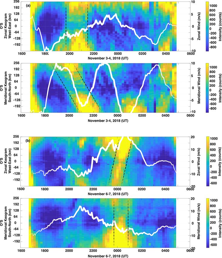
F. Vargas et al.: Gravity wave activity during the SIMONe–2018 campaign 13641
3.2 Large-scale gravity wave analysis brightness structures around 21:00 UTC (dashed black lines).
As the meridional wind fluctuation peaks, the meridional
During SIMONe–2018, we also observed the presence of keogram brightness dims (Fig. 8a bottom); as the meridional
large-scale gravity waves modulating simultaneously the air- wind fluctuation reverses direction, the airglow brightens. We
glow brightness (Fig. 1c and e) and the horizontal wind have estimated τo ∼ 4.0 ± 1.0 h for this oscillation from the
(Fig. 2c and d). To study these large-scale oscillations in the meridional wind fluctuations, where the assigned uncertainty
wind at the altitude of the airglow, we have calculated the in τo corresponds to the smallest division in the keogram tem-
wind fluctuations weighted by the volume emission rate of poral axis. The tilted brightness structure between 19:00 and
each layer using 21:00 UTC in the meridional keogram indicates a wave is
R 0 0
u , v VER dz traveling southwards. The zonal keogram shows no obvious
0 0
uw , vw = R . (3) tilt in the enhanced brightness, suggesting no wave propaga-
VER dz
tion in the east–west direction. That is confirmed from zonal
The result is seen in Fig. 6d–f, where the dashed boxes wind (Fig. 8a top) that does not show any apparent oscillation
indicate hours of simultaneous operation of the ASI and in the same time span.
MSMR systems. Similarly, we have observed enhancements in the airglow
The weighted wind fluctuations are similar in each layer as brightness on 6–7 November associated with a large-scale
the layers peak within ±2 km from each other (see Table 2) wave with τo ∼ 8.0 ± 1.0 h estimated from the wave activity
and are thicker (mean FWHM ∼ 15 km) than expected (e.g., in the zonal wind fluctuation seen in Fig. 8b top. The zonal
Greer et al., 1986; Gobbi et al., 1992; Melo et al., 1996; Wüst wind fluctuation coincides well with the O(1 S) enhanced
et al., 2017). The similarity of these fluctuations is related to brightness structure in the zonal keogram around 00:00 UTC.
larger-scale λz waves seen in Fig. 2c and d. Moreover, be- This brightness enhancement shows a slight tilt that indicates
cause the overlap of the VER profiles is non-negligible, the a wave propagating from west to east. The negligible bright-
rms values of the weighted winds fluctuations are expected ness tilt in the meridional keogram (Fig. 8b bottom) implies
to have a similar magnitude. Calculated rms magnitudes are the wave has no evident north–south component.
6.9 ± 1.0 and 5.9 ± 0.9 m s−1 in the zonal and meridional di- Spectral analysis of keograms for the two nights showing
rections, respectively. large-scale waves is shown in Fig. 9. The zonal and merid-
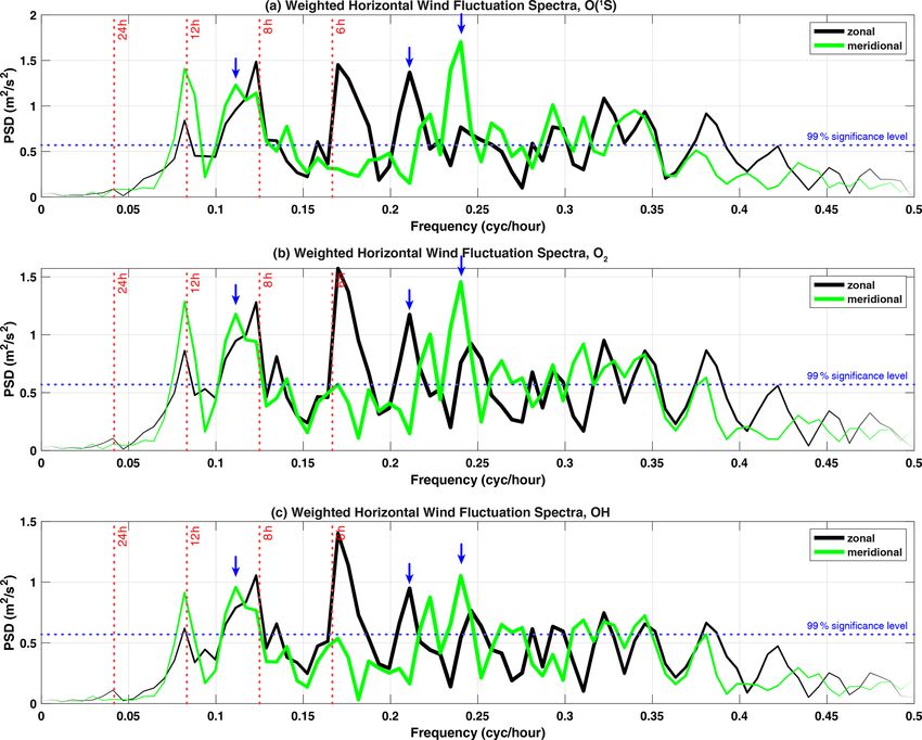
The spectral content of the weighted wind fluctuations is ional keogram spectra for 3–4 November are in Fig. 9a and c,
shown in Fig. 7. Several tidal harmonics are still present while zonal and meridional keogram spectra for 6–7 Novem-
in the spectra (vertical dotted red lines in Fig. 7). This is ber are in Fig. 9b and d. Appendix C gives further details
due to how the wind fluctuations are calculated, i.e., by about the keogram spectral analysis carried out here.
first using a 4 h temporal, 4 km vertical window to obtain For 3–4 November, the zonal keogram spectrum in-
winds representing larger scales, then subtracting the re- dicates a peak at kx = 0 and ωo = −0.17 cycles h−1
sult from the background wind. Thus, the obtained wind (τo = 5.7 ± 1.0 h), where the negative sign is associated
fluctuations will contain some of the energy of the tidal with a forward-evolving time. The meridional keogram
modes. However, there are persisting peaks attributed to spectrum shows a dominant peak at ωo = −0.21 cycles h−1
gravity waves because of their presence in wind fluctua- (τo = 4.6 ± 1.0 h) and ky ∼ −0.7 × 10⁻³ cycles km−1
tions and keograms. For instance, the peaks in Fig. 7 at the (λy ∼ 1365 ± 136 km), where the negative sign indicates a
vicinity of 0.24 cycles h−1 are seen in the wind fluctuation southward-propagating wave. The error in λy is based on
of 3–4 November (meridional direction). Likewise, Fig. 7 Vargas (2019), who estimates 10 % error in measurements
shows a peak near 0.11 cycles h−1 corresponding to a wave of large horizontal-scale waves (> 100 km) from spectral
of 8.9 ± 1.0 h also seen in the keograms of 6–7 November analysis. Note that because the horizontal scale of the wave
(zonal direction). A hodograph analysis of the winds must in the meridional direction is twice as large as the mapped
be carried out in a separate work to clarify the nature of the image field of view (FOV; 512 × 512 km2 ), the entire
significant peaks in Fig. 7. horizontal wave structure is hardly seen in a single airglow
We have studied further the wind fluctuations against ob- image but is doubtless recognized in the keogram.
vious wave features present in the keograms of 3–4 and 6– The large-scale wave occurring on 6–7 November is
7 November. By visual inspection of the images, we have represented in the zonal spectrum by the peak near
verified that these large-scale waves do not fit within the air- ωo ∼ −0.11 cycles h−1 (τo = 9.1 ± 1.0 h) and kx ∼ 0.2 ×
glow image field of view (512 × 512 km2 ) and are only no- 10−3 cycles km−1 (λx ∼ 4096 ± 409 km), where the positive
ticeable via keogram analysis. We carry out the analysis by sign indicates an eastward-propagating wave. The meridional
overlapping the O(1 S) weighted wind fluctuations on top of keogram spectrum indicates a peak at the same frequency but
the corresponding keograms for these nights (Fig. 8). ky ∼ 0, indicating no wave propagation in the meridional di-
On 3–4 November (Fig. 8a), a strong and coherent os- rection.
cillation is observed in the meridional wind fluctuation, Figure 10 shows the time–altitude cross section of the
while both zonal and meridional keograms present enhanced zonal and meridional wind fluctuations for the nights of 3–
https://doi.org/10.5194/acp-21-13631-2021 Atmos. Chem. Phys., 21, 13631–13654, 202113642 F. Vargas et al.: Gravity wave activity during the SIMONe–2018 campaign Figure 7. Spectra of weighted zonal and meridional wind fluctuation of Fig. 6. The dashed red lines indicate tidal periods. The vertical blue arrows indicate wave frequencies of persisting wave structures also seen in the airglow brightness. Statistical 99 % significance level is indicated by dotted blue lines. 4 and 6–7 November, respectively. The descending phase wave is not related to the 8 h tide since the horizontal struc- progression in time–altitude cross section reveals that these ture of the oscillation can be seen in the keogram of Fig. 8b large-scale waves are propagating upwards. We have drawn entirely. The apparent periods derived here from the de- continuous (dotted) white lines on top of the crests (troughs) scending phase analysis are consistent with those from the of the salient wave structures to estimate λz and τo of the keogram spectral analysis shown earlier. oscillations. The lines were drawn where the wave struc- tures are better defined on top of the meridional wind (3–4 November) and zonal wind (6–7 November) fluctu- 4 Discussion ation cross sections. From these lines, we have estimated λz = 25.6 ± 1.0 km and τo = 4.3 ± 1.0 h for the wave seen on The propagation conditions for gravity waves during 3–4 November. Note that the assigned error of 1 km in λz SIMONe–2018 are depicted in Fig. 4 showing the temper- corresponds to ∼ 2 times the vertical resolution of the ver- ature and constituent densities near the Kühlungsborn ob- tical axis in Fig. 10, while the assigned error of 1 h in τo servatory. While the vertical structures of the atomic oxygen corresponds to the resolution of the temporal axis in Fig. 10. density appear normal, the mean temperature indicates con- For the wave seen on 6–7 November we have obtained vectively favorable conditions for gravity wave vertical prop- τo = 8.0 ± 1.0 h and λz = 21.3 ± 1.0 km. This long-period agation as the ambient lapse rate is positive for z >∼87 km Atmos. Chem. Phys., 21, 13631–13654, 2021 https://doi.org/10.5194/acp-21-13631-2021
F. Vargas et al.: Gravity wave activity during the SIMONe–2018 campaign                                                     13643

Figure 8. Enhanced contrast keograms of O(1 S) airglow for (a) 3–4 November and (b) 6–7 November 2018. The keogram of 3–4 November
shows a large-amplitude, large-scale gravity wave at 20:00–22:00 UTC heading south. A large-scale wave is also seen on 6–7 November
propagating eastward at 00:00 UTC. The white continuous lines on the keograms indicate the wind fluctuations weighted by the O(1 S)
volume emission rate.

and z  50 m s−1 (Fig. 2a and

https://doi.org/10.5194/acp-21-13631-2021                                         Atmos. Chem. Phys., 21, 13631–13654, 2021
13644                                               F. Vargas et al.: Gravity wave activity during the SIMONe–2018 campaign

Figure 9. Composite (kx , ωo ) and (ky , ωo ) spectra of the keograms in Fig. 8 for the nights of 3–4 November (a, c) and 6–7 November (b, d).

b), the wind field could have caused absorption of waves hav-            east quadrant sector (270 to 360◦ ), while wind has a mean
ing a phase speed < 50 m s−1 traveling in the same direction             magnitude of 39.3 ± 18.9 m s−1 in the same sector (Fig. 5k.
of the background wind.                                                  This suggests these fast waves were able to overcome absorp-
   We can verify the effect of background wind on the prop-              tion levels while propagating vertically.
agation direction of the waves by examining Fig. 5. The mo-                 Horizontal and vertical wavelengths, intrinsic periods, and
mentum flux vs. propagation direction chart (Fig. 5a) shows              intrinsic phase speeds of waves detected during SIMONe–
a number of waves with large FM oriented towards the north-              2018 are directly comparable with the results of Li et al.
west and southwest, while Fig. 5k shows a dominant south-                (2011), who used a similar auto-detection method to analyze
eastward wind during SIMONe–2018 observations. Thus, it                  short-period, fast gravity waves in the airglow. Our statistics
is likely that the background wind controls the propagation              show an average λz of 18.5 ± 4.6 km (4.6 km is the sample
of southeastward waves via dynamic filtering. However, the               standard deviation), which is compatible with the results of
wave propagation direction histogram (Fig. 5f) indicates that            Li et al. (2011) showing λz clustering from 20 to 30 km. They
a significant number of waves still propagate into the wind.             have shown λh clustering around 15–30 km, while our results
These waves must then have a horizontal phase speed larger               peak around 75–100 km. Fast waves reported here present
than the background wind. In fact, we have estimated an aver-            remarkably larger horizontal scales than those of Li et al.
age ci = 56.6 ± 13.6 m s−1 for waves traveling in the south-             (2011), which could be associated with the location and type

Atmos. Chem. Phys., 21, 13631–13654, 2021                                                  https://doi.org/10.5194/acp-21-13631-2021
F. Vargas et al.: Gravity wave activity during the SIMONe–2018 campaign                                                              13645

Figure 10. Time–altitude cross section of the zonal and meridional wind fluctuations for the nights of 3–4 and 6–7 November 2018. The
continuous (dashed) white lines indicate crests (troughs) of the oscillations as well as the descending phase (ascending energy propagation)
of the waves. Note the coherent τo ∼ 4.3 h gravity wave oscillation on 3–4 November with λz ∼ 25.6 km. The zonal wind oscillation on
6–7 November corresponds to a λz ∼ 21.3 km, τo ∼ 8.0 h gravity wave.

of terrain (Maui – sea vs. Kühlungsborn – land) and gravity             Brunt–Väisälä period. The filter wheel cycle time seems to
wave sources acting near the observatories. Yet, our sample             affect other parameters as well. For instance, while Li et al.
is representative of the winter solstice conditions observed            (2011) report a majority of wave intrinsic phase speeds in
during a week, while that from Maui is representative of the            the range of 50–100 m s−1 ; we have estimated slower intrin-
season conditions observed over 5 years.                                sic phase speeds of 31.2 ± 17.3 m s−1 . The filter wheel cycle
   There are obvious discrepancies in τi estimated here com-            influences the sensitivity of the measurement system in the
pared to those of Li et al. (2011). Observe that τi here bulks          temporal domain but not the spatial domain, that is, the sys-
around 20 to 30 min, while Li et al. (2011) report 77 % of              tem will automatically detect faster waves having smaller-
waves having τi < 10 min. We attribute this discrepancy to              periods but in the same λh range.
the different integration time and the filter wheel cycle of the           In another study, Li (2011) used 1 year of OH airglow ob-
observing airglow camera systems; during SIMONe–2018,                   servations over the Andes Lidar Observatory (ALO) in South
we have observed several emissions using a filter wheel cycle           America to characterize small-scale, fast gravity waves. He
period of 10 min, which only allows us to detect waves pre-             found that the peak of distribution of λh falls in the 20–30 km
senting τo > 20 min. Li et al. (2011) used a filter wheel cycle         range, ci ranges mainly 40–100 m s−1 (peak at 70 m s−1 ),
of 2 min while observing a single emission, allowing the de-            80 % of the τi population ranges from 5–20 min, and the
tection of waves of timescales as short as ∼ 5–6 min, near the          λz distribution peaks around 15 km. These results resemble

https://doi.org/10.5194/acp-21-13631-2021                                               Atmos. Chem. Phys., 21, 13631–13654, 2021
13646                                          F. Vargas et al.: Gravity wave activity during the SIMONe–2018 campaign

those of Maui, and the same discrepancies are applicable for     O2 images, presenting larger FM since it increases as λz de-
the results in SIMONe–2018. However, the sources of waves        creases (Fig. 5i).
over the South American observatory are much clearer and            We see that even in smaller numbers, the more energetic,
related to convection in central Argentina to the east of ALO.   larger FM waves could have a greater impact in the atmo-
These sources generate fast, short-period, small horizontal-     sphere. For instance, during the Deep Propagating Gravity
scale waves that can be captured over the ALO imager.            Wave Experiment (DEEPWAVE), Bossert et al. (2015) inves-
The farther away the source, the fewer short-periods waves       tigated mountain waves presenting horizontal scales of 200–
are seen, which explains a secondary peak around λh = 80–        300 km with FM in the range of 20–105 m2 s−2 . Similarly,
100 km shown in Li (2011). This range is comparable to the       Smith et al. (2020) estimated FM ∼ 232 m2 s−2 associated
λh distribution from the SIMONe–2018 campaign showing            with an extensive and bright mesospheric gravity wave event
a peak around λh = 75–100 km that would be related to tro-       seen over the El Leoncito Observatory, Argentina (31.8◦ S,
pospheric convective sources active to the north and east of     69.3◦ W), during the nights of 17 and 18 March 2016. The
Kühlungsborn during SIMONe–2018.                                 waves observed in this study carrying FM > 3 m2 s−2 would
   The momentum flux of high-frequency waves detected            potentially cause FD ∼ 22–41 m s−1 d−1 (Vargas et al., 2007,
during SIMONe–2018 (Fig. 5) is calculated using Vargas           Fig. 9e), considering that the wave breaking continues for
et al. (2007, Eq. 13) as shown in Appendix B. The mean           24 h. This would lead to considerable mean flow decelera-
momentum flux has a larger component towards the west of         tion and body forces capable of exciting secondary waves
−0.36 ± 1.51 m2 s−2 . Note that the mean FM shows a ten-         as point-like sources (Vadas and Becker, 2018). Consider-
dency of a net wave motion westward, while the standard          ing the wave source and wave breaking mechanism acting
deviation indicates that waves could be moving westward          for 4 h (about half of a typical nighttime observation period)
or eastward. The FM meridional component is ∼ 1/6 of the         at a given altitude, we estimate a potential mean flow decel-
zonal magnitude. Ignoring for a moment the wave propaga-         eration of 3.7–6.8 m s−1 in this time span (4 h) due to wave
tion direction, the mean FM = 1.62 ± 2.70 m2 s−2 . For all the   forcing.
362 waves detected during SIMONe–2018, 50 % of the total            In a similar study, Suzuki et al. (2010) presented iden-
FM is due to waves carrying FM > 3 m2 s−2 (40 events); that      tical gravity wave structures detected in airglow intensity,
is, only 11 % of the detected waves are responsible for 50 %     radar wind, and lidar temperature. In airglow keograms from
of FM measured during the campaign. This result agrees           Northern Hemisphere stations in Japan, they observed small-
with the findings of Cao and Liu (2016) that show most of        scale gravity waves with λh ∼ 170 km, a period of 1 h propa-
FM is due to waves that occur very infrequently (low inter-      gating northeastward at ∼ 50 m s−1 . Using from both airglow
mittency). However, Cao and Liu (2016) also conclude that        images and meteor radar wind, they calculated an average
small FM waves are important because of their higher occur-      FM of 0.8 m2 s−2 at 94 km and 1.5 m2 s−2 at 86 km for the
rence rate.                                                      observed oscillations. The Suzuki et al. (2010) flux measure-
   Observe that the 362 detected events are not necessarily      ments agree with our estimates for small-scale waves that
independent, that is, the same wave could have been detected     show a majority of events carrying small FM . They have also
multiple times throughout the night. However, we rely on         estimated the acceleration of 0.8 m s−1 h−1 (19.2 m s−1 d−1 )
sets of three images to make wave detections. Since the time     at the 94 km height, which is close to our estimations of FD
span of each set is about 20 min (10 min between successive      for small-scale waves.
images), waves detected in the given set would have disap-          Ern et al. (2011) shows absolute FM values of ∼ 10−3.9 Pa
peared from the imager FOV after that time span. This is         at 50 km altitude and ∼ 10−4.3 Pa at 70 km altitude in the
because the duration of quasi-monochromatic wave packets         Northern Hemisphere in January for latitudes/longitudes
in airglow images are generally short. Thus, the same waves      near the Kühlungsborn observatory, evidencing momentum
are unlikely to be detected in multiple image sets. This way,    flux deposition in the middle atmosphere. Thus, it is likely
it would be more likely that most of the 362 detections cor-     that the small-scale waves observed here mostly dissipate as
respond to different, independent waves.                         they travel through the MLT, in agreement with Vargas et al.
   In spite of the small mean value, FM bursts between 10–       (2019). In another flux estimation study using airglow im-
30 m2 s−2 were mainly seen in the O2 emission during the         agery of gravity waves, Vargas et al. (2009) revealed FM
campaign. These waves were traveling northwestward with          ranging from ∼ 1.5 to ∼ 4.5 m2 s−2 , while radar measure-
τi = 30–40 min, λh ∼ 90 km, and λz = 12–15 km (see charts        ments of, e.g, Yuan and Fritts (1989) estimated FM = 5–
of each emission in the Supplement). The sum of FM of these      15 m2 s−2 . Also, it is believed 70 % of the momentum is
waves (eight events) accounts for 20 % of the total small-       carried by short-period waves (< 1 h) (Vincent, 1984). Es-
scale wave FM measured during the campaign. It is not clear      timations of FD (wave drag) in the meridional direction from
why the enhanced waves are seen most in the O2 emission          airglow measurements unveiled accelerations of 3 m s−1 d−1
once the layer’s peaks nearly overlap, but this could be re-     (Vargas et al., 2015), which is significant given that the
lated to the O2 VER having a narrower FWHM (see Table 2).        meridional wind magnitude is weak (∼ 20 m s−1 or less at
This way, shorter λz waves would be detected primarily in

Atmos. Chem. Phys., 21, 13631–13654, 2021                                        https://doi.org/10.5194/acp-21-13631-2021
F. Vargas et al.: Gravity wave activity during the SIMONe–2018 campaign                                                  13647

midlatitudes), while in the zonal wind the wave FD = 15–         scale, large-amplitudes waves would have a greater impact
60 m s−1 d−1 (Vincent and Fritts, 1987).                         on the mean flow than small-scale waves, even though these
   We have also estimated the horizontal wavenumber and          waves are less frequent in mesospheric measurements than
apparent frequency of the large-scale waves shown in the air-    their small-scale counterparts.
glow (Fig. 8) from the spectrum of the zonal and meridional         Gong et al. (2019) also investigate the properties of
keograms in Fig. 9. We then estimate λz of the events assum-     large-scale, long-period waves observed on 30 May 2012
ing a Brunt–Väisälä period of 5.5 min (N = 0.01904 rad s−1 )     in China. Datasets of three instruments used in the study
and an inertial period of 14.8 h (f = 0.11816×10⁻³ rad s−1 )     have shown evidences of the same gravity-wave-perturbing
for the Kühlungsborn latitude. We use the acceleration due to    lidar and SABER temperatures as well as meteor radar
gravity g = 9.5 m s−2 for the mesosphere.                        winds. The parameters associated with the observed wave
   The wave occurring on 3–4 November presents kh = ky =         are λh = 560 km, λz = 8–10 km, τo = 6.6–7.4 h, and a phase
−0.7 × 10⁻³ cycles km−1 and ωo = 0.215 cycles h−1 esti-          speed of 21 m s−1 . Gong et al. (2019) and Reichert et al.
mated from the keogram spectra. The weighted background          (2019) along with our study represent a few efforts to charac-
wind field over the observatory at 23:15 UTC presented u =       terize larger-scale gravity waves propagating from the strato-
28.5 m s−1 and v = −1.4 m s−1 at the instant the wave was in     sphere into the mesosphere using multi-instrument datasets.
the dimmer phase of its cycle in the airglow. Then applying a       According to Vargas et al. (2019), only a minority of waves
Doppler shift correction, we estimate an intrinsic frequency     seen in the airglow (∼ 5 %) are in non-dissipating regimes.
ω = 0.211 cycles h−1 for the wave. Finally, using the disper-    Vargas et al. (2019) also show that the majority of the grav-
sion relation (Appendix C), we derive λz = 25.1 ± 2.5 km         ity waves present strong dissipation and transfer momentum
for the 3–4 November wave, where the uncertainty is 20 %         flux to the main flow within a distance of two atmosphere-
as estimated in Vargas (2019). This wavelength compares          scale heights (12–14 km). Thus, the large FM waves dis-
well with λz = 25.6 ± 1.0 km obtained by visual inspection       cussed here are likely to present dissipative or breaking char-
of Fig. 10.                                                      acteristics given their larger amplitudes. This is not without
   Likewise, the 6–7 November wave has kh = kx ∼ 0.2441×         controversy, since recent radar measurements in Antarctica
10−3 cycles km−1 and ωo = 0.11 cycles h−1 . Applying once        (Sato et al., 2017) have shown longer-period gravity waves
again the Doppler shift correction using background wind         (1 h–1 d) transporting larger FM , although short-period oscil-
components of u = 26.0 m s−1 and v = −30.0 m s−1 at              lations also have significant FM but are relatively smaller.
23:26 UTC, we obtain an intrinsic frequency of ω =                  Recently, Vadas and Becker (2018) have modeled the evo-
0.087 cycles h−1 . From the dispersion relation we then es-      lution of mountain waves over the Antarctic Peninsula after
timate λz = 20.5 ± 2.0 km for this wave, which also agrees       observational results of large-scale, long-period waves seen
with the measured value of λz = 21.3 ± 1.0 km from Fig. 10.      in the mesosphere (Chen et al., 2013, 2016) attributed to
   The amplitudes of the large scale from keogram waves          an unbalanced flow in the lower stratosphere. This imbal-
are I% 0 = 36.5 % (3–4 November @ 21:30 UTC) and                 ance excited upward- or downward-propagating oscillations
I%0 = 47.9 % (6–7 November @ 00:30 UTC). These ampli-            from the knee of fish-bone-like structures at 40 km altitude,
tudes are relative to the mean airglow brightness of each        which are associated with the excitation of secondary waves
night. As demonstrated in Appendix B, the vertical wave-         from the breaking of extensive mountain wave structures. Al-
length of each wave along with their perturbations in bright-    though other modeling efforts also attribute the excitation of
ness permit us to evaluate their relative perturbation in tem-   non-primary waves to localized turbulence eddies from grav-
perature as T%0 = 9.1 % (3–4 November) and T%0 = 13.7 %          ity wave breaking (e.g., Heale et al., 2020), we believe that
(3–4 November ). Then, we finally estimate FM (see Ap-           the large-scale waves observed in this study are the prod-
pendix B) by using the intrinsic parameters found for the        uct of the Vadas and Becker (2018) mechanism at play in
observed large-scale waves, which are FM = 21.2 m2 s−2 for       the stratosphere. In fact, preliminary analysis of temperature
the wave seen on 3–4 November and FM = 29.6 m2 s−2 for           profiles at 0–90 km altitude acquired by the IAP Rayleigh li-
that seen on 6–7 November. Table 3 shows a summary of the        dar system on 6–7 November revealed fish bone structures at
main features of the large-scale waves as discussed above.       40–45 km, resembling the predictions of Vadas and Becker
We expect the uncertainties in FM to be large (> 40 %) given     (2018). We will investigate in detail the possible connec-
that the FM variables incur in uncertainties that are trans-     tion with the large-scale waves seen here in a separate paper;
ferred to FM via error propagation (Vargas, 2019).               specifically, we want to identify potential sources of primary
   Based upon FM values of the large-scale waves, we es-         waves in the vicinity of Kühlungsborn during SIMONe–2018
timate for the southward-traveling wave (3–4 November) a         and also trace the observed large-scale waves back to their
momentum flux divergence FD ∼ 43 m s−1 d−1 in the merid-         excitation altitude around the fish bone knee region at 40–
ional flow, assuming this wave breaks or dissipates at a given   45 km revealed in the filtered lidar temperatures.
level along its vertical path. Similarly, the 6–7 November
wave would cause a deceleration of FD ∼ 38 m s−1 d−1 in the
zonal flow at the breaking or dissipation level. These large-

https://doi.org/10.5194/acp-21-13631-2021                                      Atmos. Chem. Phys., 21, 13631–13654, 2021
You can also read