Diurnal cycle of coastal anthropogenic pollutant transport over southern West Africa during the DACCIWA campaign
←
→
Page content transcription
If your browser does not render page correctly, please read the page content below
Atmos. Chem. Phys., 19, 473–497, 2019
https://doi.org/10.5194/acp-19-473-2019
© Author(s) 2019. This work is distributed under
the Creative Commons Attribution 4.0 License.

Diurnal cycle of coastal anthropogenic pollutant transport over
southern West Africa during the DACCIWA campaign
Adrien Deroubaix1,2 , Laurent Menut1 , Cyrille Flamant2 , Joel Brito9 , Cyrielle Denjean6 , Volker Dreiling7 ,
Andreas Fink5 , Corinne Jambert4 , Norbert Kalthoff5 , Peter Knippertz5 , Russ Ladkin8 , Sylvain Mailler1 ,
Marlon Maranan5 , Federica Pacifico4 , Bruno Piguet6 , Guillaume Siour3 , and Solène Turquety1
1 LMD/IPSL,    Laboratoire de Météorologie Dynamique, Ecole Polytechnique, IPSL Research University,
Ecole Normale Supérieure, Université Paris-Saclay, Sorbonne Universités, UPMC Univ Paris 06, CNRS,
Route de Saclay, 91128 Palaiseau, France
2 LATMOS/IPSL, Sorbonne Université, Université Paris-Saclay & CNRS, Paris, France
3 LISA/IPSL, Laboratoire Interuniversitaire des Systèmes Atmosphériques (LISA), UMR CNRS 7583,

Université Paris Est Créteil et Université Paris Diderot, Institut Pierre Simon Laplace, Créteil, France
4 LA, Laboratoire d Aérologie, University of Toulouse, CNRS, UPS, Toulouse, France
5 KIT, Institute of Meteorology and Climate Research, Karlsruhe Institute of Technology, Germany
6 CNRM, Centre National de la Recherche Météorologique, UMR3589, CNRS, Météo-France, Toulouse, France
7 DLR, Deutsches Zentrum für Luft- und Raumfahrt, Oberpfaffenhofen, Germany
8 BAS, British Antarctic Survey, Cambridge, UK
9 LAMP, Laboratoire de Météorologie Physique, Université Clermont Auvergne, Aubière, France

Correspondence: Adrien Deroubaix (adrien.deroubaix@lmd.polytechnique.fr)

Received: 25 July 2018 – Discussion started: 3 August 2018
Revised: 15 November 2018 – Accepted: 9 December 2018 – Published: 14 January 2019

Abstract. During the monsoon season, pollutants emitted           of Cotonou (Benin). Numerical model experiments indicate
by large coastal cities and biomass burning plumes origi-         that the anthropogenic pollutants are accumulated during the
nating from central Africa have complex transport pathways        day close to the coast and transported northward as soon as
over southern West Africa (SWA). The Dynamics–Aerosol–            the daytime convection in the atmospheric boundary layer
Chemistry–Cloud Interactions in West Africa (DACCIWA)             ceases after 16:00 UTC, reaching 8◦ N at 21:00 UTC. When
field campaign has provided numerous dynamical and chem-          significant biomass burning pollutants are transported into
ical measurements in and around the super-site of Savè in         continental SWA, they are mixed with anthropogenic pollu-
Benin ( ≈ 185 km away from the coast), which allows quan-         tants along the coast during the day, and this mixture is then
tification of the relative contribution of advected pollutants.   transported northward. At night, most of the coastal anthro-
Through the combination of in situ ground measurements            pogenic plumes are transported within the planetary bound-
with aircraft, radio-sounding, satellite, and high-resolution     ary layer (below about 500 m above ground level), whereas
chemistry-transport modeling with the CHIMERE model,              the biomass burning pollutants are mostly transported above
the source attribution and transport pathways of pollutants       it, thus generally not impacting ground level air quality.
inland (here, NOx and CO) are carefully analyzed for the
1–7 July 2016 period. The relative contributions of different
sources (i.e., emissions from several large coastal cities) to
the air quality in Savè are characterized. It is shown that a
systematic diurnal cycle exists with high surface concentra-
tions of pollutants from 18:00 to 22:00 UTC. This evening
peak is attributed to pollution transport from the coastal city

Published by Copernicus Publications on behalf of the European Geosciences Union.
474                                      A. Deroubaix et al.: Diurnal urban pollution transport over southern West Africa

1   Introduction                                                   sions, or they focused on sampling BB aerosol layers (Fla-
                                                                   mant et al., 2018b). The DACCIWA field campaign took
The United Nations Department of Economic and Social Af-           place in so-called post-WAM post-onset conditions, i.e., af-
fairs, Population Division reported 31 megacities globally         ter deep convection (and related precipitation) had migrated
(urban agglomerations with more than 10 million inhabitants        from the coast inland over the Sahel (Knippertz et al., 2017).
in 2016) and that their number is projected to rise up to 41          During the WAM, the atmospheric composition over the
by 2030. In southern West Africa (SWA), Lagos is consid-           Gulf of Guinea coastal region is the result of a complex mix
ered a megacity (with more than 13 million inhabitants) and        of natural and anthropogenic sources, which include urban,
is expected to reach 24 million in 2030. The urban agglom-         BB, biogenic, desert dust, and oceanic compounds. Using nu-
eration extends along the coast to Cotonou (Benin) and even        merical tracer experiments, Menut et al. (2018) have high-
to Lomé (Togo). Moreover Accra in Ghana (with a popu-              lighted that fire emissions in central Africa impacting the
lation predicted to increase from 2.3 in 2016 to 3.3 million       surface aerosol and gaseous species concentrations over the
in 2030), Kumasi in Ghana (with a population predicted to          Gulf of Guinea are mostly transported over the southeast At-
increase from 2.7 in 2016 to 4.2 million in 2030) and Abid-        lantic above the marine PBL. Using WRF–CHIMERE nu-
jan in Côte d’Ivoire (with a population predicted to increase      merical simulations of the WAM during the African Mon-
from 5.0 in 2016 to 7.8 million in 2030) will all contribute       soon Multidisciplinary Analyses (AMMA) campaign period
to form a more or less continuously urbanized strip at some        from May to July 2006, Deroubaix et al. (2018) quantified
point during the twenty-first century. This growth is asso-        the relative contributions of anthropogenic and BB sources
ciated with enhanced pollutant emissions and low air qual-         to carbon monoxide (CO) concentrations over SWA, which
ity, which leads to chronic health problems (Lelieveld et al.,     in July 2006 were about 25 % local anthropogenic and 50 %
2015) and contributes to anthropogenically forced climate          BB from central Africa. The remaining 25 % are the back-
change.                                                            ground corresponding to long-range transport from outside
   The vertical structure of air pollution is complex along the    of Africa. In order to better distinguish the contributions from
Guinea coast during the period when the West African mon-          different sources to background concentrations, additional
soon (WAM) is established in the boreal summer. From the           studies are needed focusing on Africa as has been carried
surface to the top of the planetary boundary layer (PBL),          out for other regions (e.g., Kulkarni et al., 2015; Yang et al.,
marine air transported by the northeastward monsoon flow           2017; Sobhani et al., 2018). However the high BB contribu-
gets enriched with anthropogenic pollution emitted at the          tion is partly due to the significant underestimation of an-
coast before moving further inland (Knippertz et al., 2015b).      thropogenic emissions for the Gulf of Guinea region (Marais
Above the marine PBL, biomass burning (BB) aerosol lay-            et al., 2014; Marais and Wiedinmyer, 2016; Liousse et al.,
ers, resulting from incomplete combustion of fires in cen-         2017; Keita et al., 2018).
tral Africa (Giglio et al., 2006; Zuidema et al., 2016), can          AMMA was focused on the Sahelian region combining a
on occasion be observed reaching the Guinea coast after be-        multi-scale approach to better characterize the interactions
ing transported over thousands of kilometers (Menut et al.,        among atmosphere, land, and ocean during the monsoon
2018). In higher layers, at altitudes from 3 to 5 km, the Sa-      (Janicot et al., 2008; Redelsperger et al., 2006), whereas the
haran air layer (SAL) is generally observed to be advected         DACCIWA project is dedicated to the interactions among
from the north depending on the meridional disturbances            aerosols, clouds, and radiation along the highly urbanized
of the African easterly jet (AEJ), carrying desert dust (Fla-      coastline of the Gulf of Guinea (Knippertz et al., 2015a).
mant et al., 2009; Crumeyrolle et al., 2011; Lafore et al.,        Over SWA, Adler et al. (2017) and Deetz et al. (2018) have
2011). This general picture is often perturbed by the presence     documented a regular occurrence of a coastal front, which
of organized convective systems, which propagate along the         is located where the strongest horizontal gradients of wind
Guinea coast from Nigeria to Liberia (Maranan et al., 2018).       speed and potential temperature occur. It develops during
The latter authors also note the presence of land–sea breeze       the daytime and propagates inland in the evening. After
convective systems in the immediate coastal strip.                 the frontal passage, the wind in the lowermost troposphere
   The EU-funded project Dynamics–Aerosol–Chemistry–               brings air masses, and probably also anthropogenic pollu-
Cloud Interactions in West Africa (DACCIWA) was designed           tants emitted from coastal urban areas (e.g., Djossou et al.,
to focus specifically on the Guinea coastal atmospheric dy-        2018) and BB pollutants imported by monsoon flow (e.g.,
namics and the interactions among aerosols, chemistry, and         Reeves et al., 2010), from the coast northward, especially at
clouds (Knippertz et al., 2015a). An intensive measurement         night with the nocturnal low-level jet (NLLJ) (Schuster et al.,
campaign took place in Nigeria, Benin, Togo, Ghana, and            2013).
Côte d’Ivoire during June–July 2016, which corresponds to             The main objective of this article is to understand the diur-
the climatological onset period of the WAM (Janicot et al.,        nal cycle of anthropogenic pollutant transport from the coast
2008). Three research aircraft flew over the Guinea coastal        to the continental SWA. We present numerical tracer experi-
region with different scientific objectives, notably with flight   ments made with high-resolution CHIMERE simulations set
plans designed to map out city, shipping, and flaring emis-        up in order to separate the contribution of each important ur-

Atmos. Chem. Phys., 19, 473–497, 2019                                                www.atmos-chem-phys.net/19/473/2019/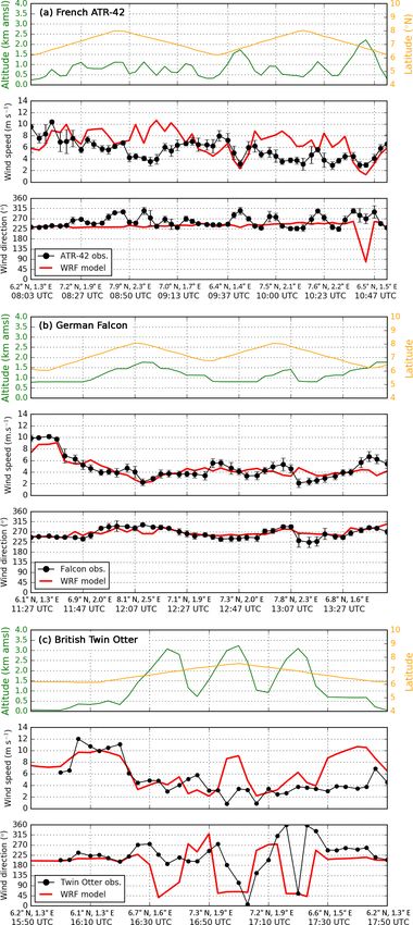
A. Deroubaix et al.: Diurnal urban pollution transport over southern West Africa                                                      475

Table 1. Characteristics of the studied cities with country, latitude, longitude, elevation above mean sea level (a.m.s.l.), and number of
inhabitants of urban agglomerations. The population in bold is given for the year 2015 according to the World Urbanization Prospects report
(United Nations report, 2011). National general population and habitat census is used to estimate the population of Cotonou and Savè (INSAE
report, 2015).

                       City       Country          Latitude    Longitude       Elevation        Number of inhabitants
                       Abidjan    Côte d’Ivoire    5.36◦ N     4.00◦ W         50 m a.m.s.l.               4 923 000
                       Accra      Ghana            5.60◦ N     0.19◦ W         30 m a.m.s.l.               3 013 000
                       Lomé       Togo             6.17◦ N     1.23◦ E         10 m a.m.s.l.               1 830 000
                       Cotonou    Benin            6.36◦ N     2.38◦ E         10 m a.m.s.l.               2 194 000
                       Savè       Benin            8.03◦ N     2.49◦ E         130 m a.m.s.l.                 87 000
                       Lagos      Nigeria          6.49◦ N     3.36◦ E         10 m a.m.s.l.              13 121 000

ban agglomeration, namely Abidjan, Accra, Lomé, Cotonou,                 2     DACCIWA project: observations and modeling
and Lagos. We take advantage of the DACCIWA measure-
ments made by the three research aircraft, by an enhanced                In the DACCIWA project, there are strong components on
radio-sounding network, and at the super-site of Savè in cen-            both in situ observations and modeling. Here, we present
tral Benin (Knippertz et al., 2015a). The super-site of Savè             all studied sites (Sect. 2.1), observational datasets used
is a representative location to assess the impact of pollution           (Sect. 2.2), and numerical simulations performed to analyze
transport from the coast on the air quality of remote inland             the pollution transport pathways (Sect. 2.3).
cities characterized by low local emissions. We focus on the
period of 1–7 July 2016, during which a case of long-range               2.1    Studied sites
transport of BB aerosol from central Africa was observed
                                                                         We focus on six locations, five major urban agglomerations
(Flamant et al., 2018b). We aim at answering the following
                                                                         of the Guinean coastal region, and one small town, Savè,
questions:
                                                                         which is 185 km north of Cotonou (Benin). Table 1 shows the
  – What is the relative contribution of each coastal urban              coordinates and the population of the urban agglomerations
    area to the air pollution at Savè? How does it evolve                studied. For Abidjan, Accra, Lomé, and Lagos, we present
    during the day?                                                      estimations for the year 2015 of the department of social and
                                                                         economic affairs of United Nations (United Nations report,
  – How are BB and anthropogenic pollutants mixed along                  2011). In this report, these cities are associated with large
    the coast and inland? Is it usually a mixture of the two             administrative areas in contrast to Cotonou.
    pollution types that is transported inland in the PBL?                  Comparing Lomé and Cotonou, Lomé has a large admin-
                                                                         istrative area while Cotonou is a city with a very high popu-
   This study is focused on one specific period and location.
                                                                         lation density over a small area. The population of Lomé is
However, the conclusions are representative of a longer time
                                                                         about 839 000 inhabitants in the city according to the gen-
period as meteorological conditions at the coast during the
                                                                         eral population and habitat census of Togo (DGSCN report,
so-called monsoon post-onset period were found to be quite
                                                                         2016) and about 1 830 000 inhabitants in the administrative
stable for several weeks (Knippertz et al., 2017). Spatially,
                                                                         state (United Nations report, 2011). Cotonou city is estimated
the results are directly representative of the studied region
                                                                         by the World Urbanization Prospects report to have about
only, the main goal being to estimate the influence of the
                                                                         1 086 000 inhabitants (United Nations report, 2011).
emissions from four coastal cities on the atmospheric compo-
                                                                            According to the general population and habitat census of
sition in the lower troposphere over inland Benin. Given the
                                                                         Benin (INSAE report, 2015), the population of Cotonou only
broad southwesterly monsoon flow in the region, a similar
                                                                         slightly increased by 2.09 % over the period of 2002–2013
transport from coastal pollution inland will likely be found
                                                                         because of the limited possibility of expansion. They note
along most of the Guinea coast. We shall answer these ques-
                                                                         that along the shores of Lake Nokoué the population has in-
tions using a synergistic combination of observations and
                                                                         creased rapidly, thus forming an agglomeration of 2 194 000
numerical modeling experiments, described in Sect. 2. Sec-
                                                                         inhabitants, calculated as the sum of the Cotonou district
tion 3 analyzes the temporal evolution of meteorology and
                                                                         and several cities of the Atlantique district (Abomey-Calavi
air pollution over a portion of SWA including Côte d’Ivoire,
                                                                         and Sô-Ava) and of the Ouémé district (Sèmè Kpodji, Porto
Ghana, Togo, Benin, and Nigeria. Then, we focus on urban
                                                                         Novo, Avrankou, and Akpro-Missérété).
anthropogenic (URB) and long-range BB pollutant transport
in Sect. 4. Conclusions are given in Sect. 5.

www.atmos-chem-phys.net/19/473/2019/                                                            Atmos. Chem. Phys., 19, 473–497, 2019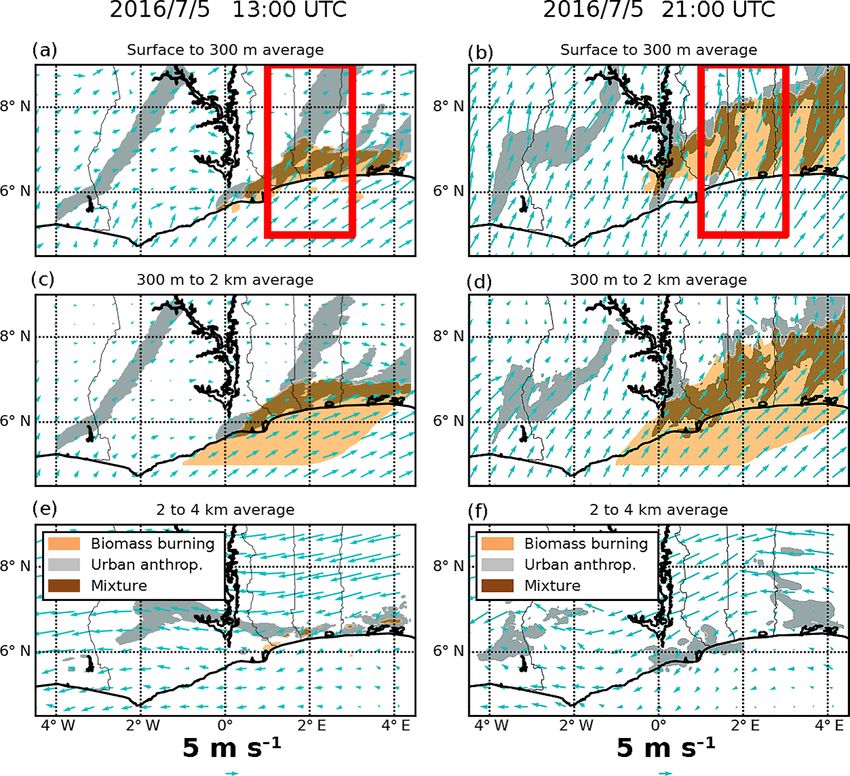
476                                           A. Deroubaix et al.: Diurnal urban pollution transport over southern West Africa

                                                                          18:00 to 21:00 UTC, the wind direction was shifted, which
                                                                          corresponds to local pollution. This period has been removed
                                                                          from the analysis.
                                                                             The DACCIWA aircraft campaign took place during the
                                                                          period of 25 June–14 July 2016 and was based at the Lomé
                                                                          (Togo) airport (Flamant et al., 2018b). Three research aircraft
                                                                          were involved: a Twin Otter operated by the British Antarc-
                                                                          tic Survey (BAS), an ATR 42 operated by the French Service
                                                                          des Avions Français Instrumentés pour la Recherche en En-
                                                                          vironment (SAFIRE), and a Falcon operated by the German
                                                                          Deutsches Zentrum für Luft- und Raumfahrt (DLR). We base
                                                                          our study on three variables, namely relative humidity (RH),
                                                                          wind direction, and wind speed, which are measured by core
Figure 1. Map of the modeling domain (red rectangles) with lo-            meteorological instrumentation. The flight trajectories used
cation of the major cities (red dots), of the Lomé airport, and of        are depicted in Fig. 1. For the three aircraft, raw observations
the Savè super-site (white dots). Superimposed are the flight tracks      acquired at 1 Hz are averaged over 3 min time steps.
of the three research aircraft during the 1–7 July 2016 period (gray
                                                                             The DACCIWA project included a large radiosonde com-
lines). The aircraft flight tracks on 5 July are colored for the German
                                                                          ponent with locations carefully chosen building on the
Falcon (blue line), the French ATR 42 (violet line), and the British
Twin Otter (yellow line).                                                 AMMA radiosonde campaign experiences (Lothon et al.,
                                                                          2008; Parker et al., 2008; Fink et al., 2011; Schuster et al.,
                                                                          2013). We use radiosondes launched from four locations:
                                                                          Abidjan, Accra, Cotonou, and Savè (see Table 1). There were
2.2   Observational datasets                                              four releases per day at around 00:00, 06:00, 12:00, and
                                                                          18:00 UTC. In Savè, more radiosondes were launched every
During the DACCIWA field campaign, several observational                  1.5 to 3 h at the super-site during the intensive observation
platforms were deployed to perform in situ and remote-                    period of 1–7 July 2016 (Kalthoff et al., 2018).
sensing measurements (Knippertz et al., 2017; Flamant et al.,                We analyze the horizontal spatial extent of the main
2018b). In this study, we use datasets acquired by ground-                aerosol plumes from satellite observations of aerosol
based stations, aircraft, radiosondes, and satellites. Table 2            optical depth (AOD) at 550 nm made by MODIS
gives the main information on each dataset. Figure 1 presents             (Moderate        Resolution      Imaging      Spectroradiometer)
the location of the aircraft flight tracks and of the stations.           on both the Aqua platform (MYD08-D3-6 dataset
Our studied domain is located in the Greenwich mean time                  DOI:        https://doi.org/10.5067/MODIS/MYD08_D3.061,
(GMT). Hence local time is the same as UTC. During the air-               passing over the studied region at 13:30 UTC)
craft campaign period, sunrise occurred around 06:00 UTC                  and the Terra platform (MOD08-D3-6 dataset DOI:
and sunset around 18:00 UTC.                                              https://doi.org/10.5067/MODIS/MOD08_D3.061, passing
   Three super-sites have been implemented in the frame-                  over the studied region at 10:30 UTC). Daily MODIS AOD
work of the DACCIWA project in Kumasi (Ghana), Ile-Ife                    averages at 1◦ resolution have been calculated from the
(Nigeria), and Savè (Benin). Unlike the two others, Savè is               Collection 6 combined product of the Dark Target retrieval
representative of transport-related air quality issues affect-            available over oceans or non-bright continental surface and
ing small cities, characterized by low local emissions, down-             the Deep Blue retrieval available over deserts (Hsu et al.,
stream of large coastal cities. It is ideal in that the terrain is        2013; Sayer et al., 2013, 2014).
very flat with no orographically induced circulation impact-                 In order to identify the altitude of aerosols together with
ing the monsoonal flow. Thus to study NOx and CO from                     their speciation, we use the spaceborne Cloud-Aerosol Lidar
coastal urbanized areas, this rural environment is well suited.           with Orthogonal Polarization (CALIOP) aerosol type classi-
   At Savè, the Karlsruhe Institute of Technology (KIT) and               fication (Winker et al., 2009). This classification is suited and
the Paul Sabatier University (UPS) have set up meteoro-                   accurate to distinguish homogenous aerosol plumes with dif-
logical and atmospheric composition measurements. UPS                     ferent optical properties such as sea salt, dust, and BB (e.g.,
installed a chemical analyzer (ThermoEnvironment instru-                  Menut et al., 2018). The CALIOP cross sections are very use-
ment), which measured NO2 , NO, and CO surface concen-                    ful since this is a realistic way to have an instantaneous evalu-
trations (Pacifico et al., 2018; Kalthoff et al., 2018). Raw              ation of the aerosol layer altitudes, with their type depending
observations acquired at 10 s are averaged hourly. The de-                on backscattered optical measurements, (e.g., Winker et al.,
tection limit of the instrument is 0.05 ppb for NO2 and NO                2013). Data are available on https://www-calipso.larc.nasa.
and 12 ppb for CO (Derrien and Bezombes, 2016). The mea-                  gov/ (last access: 10 January 2019).
surement site is upwind of Savè city when the wind corre-
sponds to the monsoon flow (SW sector). On 3 July from

Atmos. Chem. Phys., 19, 473–497, 2019                                                        www.atmos-chem-phys.net/19/473/2019/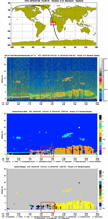
A. Deroubaix et al.: Diurnal urban pollution transport over southern West Africa                                                      477

Table 2. Datasets used in this study with acquisition platform, variables, and sampling frequency.

        Datasets               Platform                                       Variables                  Frequency
        Ground-based station   Savè super-site (8.03◦ N, 2.49◦ E)             NO2 , NO,                  Raw data: 1 hz
                               operated by KIT–UPS universities               and CO concentrations      Presented: hourly averages
        Aircraft               ATR 42, Twin Otter, Falcon                     Relative humidity          Raw data: 1 hz
                               operated by SAFIRE, BAS, and DLR teams         Wind direction and speed   Presented: 3 min averages
        Radiosonde             Launch sites:                                  Wind direction and speed   High resolution 1 hz
                               Abidjan, Accra, Cotonou, Savè                  Relative humidity          Presented: 100 m averages
        Satellite              MODIS on Terra                                 AOD (550 nm)               Daily
                               and Aqua                                       level 3 (1◦ × 1◦ )

2.3     Numerical modeling by WRF–CHIMERE models                         proximation (McICA) method of random cloud overlap from
                                                                         Mlawer et al. (1997), the PBL physics are computed using
The WRF–CHIMERE simulations presented in this study                      the Yonsei University scheme (Hong et al., 2006), the cumu-
have a setup similar to those used by Deroubaix et al.                   lus parametrization is the ensemble Grell–Dévényi scheme
(2018). Both models are run offline in a nested configura-               (for the high-resolution domain, convective precipitation is
tion on the same grids with two domains: a regional do-                  explicitly calculated and not parametrized), the surface layer
main (10 km × 10 km, extending from 1◦ S to 14◦ N and                    scheme is the Carlson–Boland viscous sublayer, and the sur-
from 11◦ W to 11◦ E) and a high-resolution coastal domain                face physics is calculated with the Noah land surface model
(2 km × 2 km). The simulations over the regional domain are              scheme with four soil temperatures and moisture layers (Ek
started on 1 June 2016. In the following, we present only                et al., 2003). This setup has already been used by Deroubaix
results modeled over the high-resolution domain (Fig. 1).                et al. (2018) because it allows the reproduction of a satis-
The simulated period over the high-resolution domain (1 to               factory diurnal cycle of wind speed over SWA according to
7 July) is entirely included in the 2016 WAM post-onset                  Schuster et al. (2013).
phase, which has been defined from 22 June to 20 July 2016
by Knippertz et al. (2017).
                                                                         2.3.2   Gaseous tracers transport from the
2.3.1     Meteorological fields from the WRF model                               CHIMERE model

Meteorological variables are modeled with the regional non-              CHIMERE is a regional chemistry-transport model (ver-
hydrostatic WRF model (version 3.7.1, Skamarock and                      sion 2017), fully described in Menut et al. (2013) and Mailler
Klemp, 2008). The domains have a constant horizontal res-                et al. (2017). The 32 vertical levels of the WRF model are
olution with 32 vertical levels from the surface to 50 hPa,              projected onto the 20 levels for CHIMERE from the surface
including about 10 vertical levels below 1 km a.m.s.l. We use            and up to 200 hPa.
a two-way nesting for the communication between different                   In this study, the model is used in its tracer version and
domains.                                                                 there is no atmospheric chemistry. We choose to release pas-
   Global meteorological fields are taken from the US                    sive gaseous tracers in the simulation because we want to
Global Forecast System (operational final analyses) pro-                 analyze only their transport (no chemistry, no deposition)
duced by the National Center for Environmental Prediction                caused by the monsoonal flow. Since we want to distinguish
(ds083.3 dataset DOI: https://doi.org/10.5065/D65Q4T4Z).                 the relative contribution of several coastal cities from the
These fields are used to provide meteorological initial and              pollution further inland, we designed a first experiment for
boundary conditions and to nudge hourly fields of pressure,              which we impose the tracer emissions at specific urbanized
temperature, humidity, and wind in the WRF simulations,                  locations: Abidjan (Côte d’Ivoire), Accra (Ghana), Lomé
with spectral nudging, which has been evaluated for regional             (Togo), Cotonou (Benin), and Lagos (Nigeria) (see Table 1
models by von Storch et al. (2000). In order to enable the               for coordinates). Specific tracers are emitted for a given city
PBL variability to be resolved by WRF, low-frequency spec-               in order to distinguish their relative contributions at inland
tral nudging is used only above 850 hPa.                                 locations. Thus the tracer emissions occur in a single grid
   The WRF model setup is as follows: the microphysics                   cell corresponding to the center of each city.
scheme is the WRF Single-Moment 6-class Microphysics                        The tracer emissions are constant and continuous during
Scheme (WSM6), the radiation scheme is the Rapid Ra-                     the modeled period (1–7 July). This allows the quantification
diative Transfer Model for General Circulation Models                    of the variability due to the meteorology only. Emissions are
(RRTMG) with the Monte Carlo independent column ap-                      released at the lowest level of the model (below 10 m in alti-

www.atmos-chem-phys.net/19/473/2019/                                                          Atmos. Chem. Phys., 19, 473–497, 2019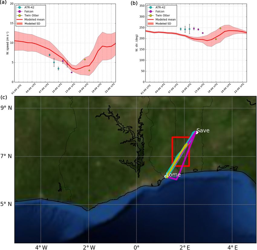
478 A. Deroubaix et al.: Diurnal urban pollution transport over southern West Africa
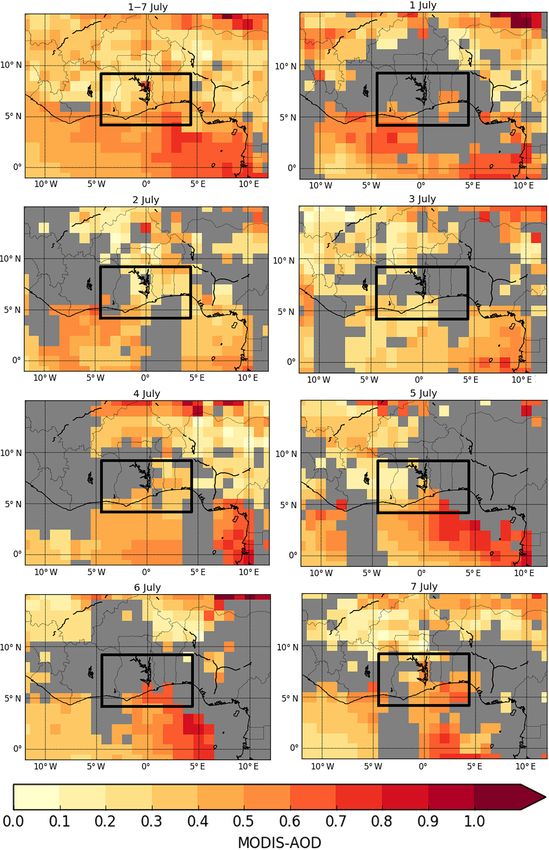
Figure 2. MODIS AOD 1-day moving average of two products acquired by Aqua and Terra (the combined Dark Target and Deep Blue
MYD08-D3 and MOD08-D3 products, respectively) on 3 July 2016 (a) and 5 July 2016 (b). Data excluded by the cloud screening process
are in gray. The modeling domain is presented by the black square.
tude) and are proportional to the population of each city; this sidered negligible in this study focused on a few days and
approach has also been used by Flamant et al. (2018a). We a spatially restricted region: it is assumed that gaseous and
defined an arbitrary emission for 1 million inhabitants. Then aerosol species are transported in the same way by the mete-
we multiply this emission by a factor depending on the pop- orological flow.
ulation (see Table 1): 1.8 for Lomé, 2.2 for Cotonou, 3 for
Accra, 5 for Abidjan, and 13 for Lagos.
A second objective is to understand the interactions be- 3 Large-scale atmospheric patterns over the Gulf of
tween urban (URB) and BB pollutants resulting from long- Guinea
rang transport on 5 July. For this, we design a second nu-
merical tracer experiment in which BB tracers are added to This section is dedicated to analysis of the atmospheric dy-
the URB tracers and are tagged to be different from the URB namics, thermodynamics, and composition across SWA us-
tracers. BB tracers are released to reproduce the BB layer ing AOD from satellites in Sect. 3.1, together with RH and
observed with MODIS on 5 July at 00:00 UTC to 6 July at wind from radiosondes in Sect. 3.2 and from aircraft in
23:00 UTC with a spatial horizontal extent going from 1◦ W Sect. 3.3. The prerequisite to realistic numerical tracer ex-
to 2◦ E at 4.5◦ N and at an altitude of ≈ 1.5 km (see Fig. 9 periments is the accuracy of the meteorological simulation.
and Sects. 3.1 and 4.3 for justifications). The WRF meteorological simulation is therefore extensively
The two tracer experiments are summarized in Ta- compared to in situ observations made by both radiosondes
ble 3. They are accessible on the DACCIWA database and aircrafts.
(https://doi.org/10.6096/BAOBAB-DACCIWA.1760, Der-
oubaix, 2018a). 3.1 Regional-scale aerosol distribution
The tracers are transported using the van Leer scheme (van
Leer, 1979). There is no sink for tracers (no deposition and This section investigates the daily MODIS AOD observa-
no chemical reaction). The tracers are chosen to be gaseous tions for the period of 1 to 7 July 2016. Two important types
and are representative of the gaseous part of the URB emis- of aerosols can be advected towards SWA: dust from the
sions and the BB plume. This choice of gaseous tracers was north and BB from the south. We focus on two different days,
made to be consistent with the gaseous concentrations mea- 3 and 5 July 2016 (Figs. 2 and A1). Note that we present 1-
sured by the aircraft and the surface gaseous concentrations day moving averages (Figs. 2) because we analyze the long-
measured at the Savè super-site. The period is not associ- range transport of aerosols (using the MODIS level 3 product
ated with widespread rain. At Savè, there were only some with a coarse resolution of 1◦ ).
small precipitation events (Kalthoff et al., 2018). We focus During the studied period, high AOD values are found
our analysis on gaseous species but we suppose similar trans- north of the domain over the Sahel (north of 14◦ N) and
port patterns for aerosol and gaseous pollutants because of south of the domain over the Gulf of Guinea (on average
the constant monsoon flow blowing over SWA during our over the period of 1–7 July, Fig. A1). The origin of the high
studied period. The only difference from aerosol is the ab- AOD over the Gulf of Guinea is well known. This is the
sence of settling. But this long-term impact could be con- BB layer coming from central Africa, where intense veg-
etation fires occur during this season (Giglio et al., 2006)
Atmos. Chem. Phys., 19, 473–497, 2019 www.atmos-chem-phys.net/19/473/2019/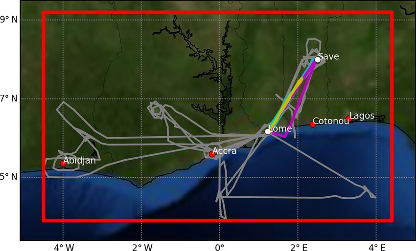
A. Deroubaix et al.: Diurnal urban pollution transport over southern West Africa 479
Table 3. Main characteristics of the two numerical tracer experiments using high-resolution modeling at 2 km grid spacing with tracer
emissions relevant for biomass burning (BB) and urban pollutants (URB).
Tracer Experiment 1 Tracer Experiment 2
Tracer type URB tracers only BB and URB tracers
Release duration 1–7 July 5–7 July (BB) and 1–7 July (URB)
Release altitude lowest level at 1500 m (BB) and lowest level (URB)
Release location five cities from 1◦ W to 2◦ E at 4.5◦ N (BB) and five cities (URB)
Number of tracer five (each city) two (BB and URB)
with increasing trends over the period of 2001–2012 (An- and observed dynamical and thermodynamical variables are
dela and Van Der Werf, 2014). Part of this pollution is trans- compared in order to identify the different layers. The mod-
ported over the Gulf of Guinea and the BB plume reaches the eled variables have been interpolated along the balloon tra-
Guinea coast, as seen during the AMMA campaign (Sauvage jectories and aircraft flight tracks using a spatial bilinear in-
et al., 2005; Reeves et al., 2010). The BB pollutant concen- terpolation and then temporal and vertical linear interpola-
trations observed along the Guinea coast depend on the syn- tions with a 3 min time step.
optic wind patterns (Menut et al., 2018). The presence of this
layer is confirmed over the Gulf of Guinea using CALIPSO 3.2.1 Identification from radiosondes
data acquired on 5 July (Fig. A2), which gives a layer al-
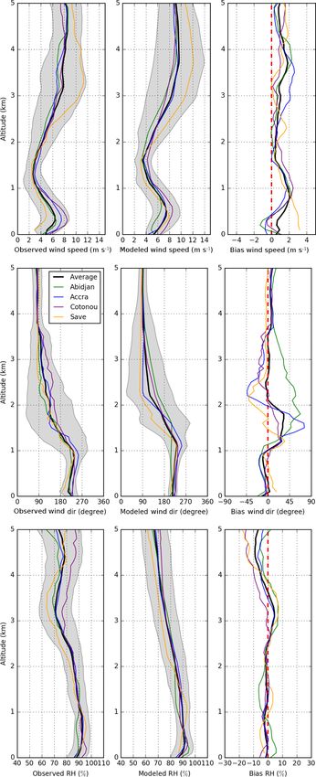
titude between 1 and 3 km above mean sea level (a.m.s.l.). For wind speed, the vertical profiles observed at the four lo-
It is worth noting that during this period, there is no evi- cations have a similar shape (Fig. 3). The mean wind speed
dence of mineral dust transport over the studied cities. The increases from the surface to 300 m a.m.s.l., then decreases to
dates 3 and 5 July 2016 are two contrasting days in terms 3 m s−1 at 1.5 km a.m.s.l. and finally increases to a maximum
of AOD values over the Gulf of Guinea (Fig. 2). On 2 July, of about 8 m s−1 between 3 and 5 km a.m.s.l. The model pre-
AOD values are low over the continent and moderate over dicts a vertical wind profile in good agreement with obser-
the ocean (Fig. A1), which is in agreement with Flamant vations from the surface to 300 m a.m.s.l. but there is an in-
et al. (2018a), who have shown that the BB layer is present creasing positive bias from 300 m to 1 km a.m.s.l., reaching
close to the Guinea coast but it does not reach the coast. On +2 m s−1 at 1 km a.m.s.l. At 300 m a.m.s.l., observed wind
3 July, AOD values are low to moderate over our domain speed reaches 6 m s−1 on average, which shows the NLLJ
(AOD < 0.5, Fig. 2). On 4 July, there is a pattern of high signature (Schuster et al., 2013). The model reproduces
AOD (AOD > 0.5) 100 km south of the coast (Fig. A1). On this signature with wind speed reaching 7 m s−1 but over-
5 July, the BB layer reaches the coastline (Fig. 2), then on estimates its altitude (at 400 m a.m.s.l.) at the three coastal
6 July it seems to penetrate inland but clouds prevent AOD sites (Abidjan, Accra, Cotonou).
retrievals over Togo and Benin (Fig. A1). On 7 July, this layer The vertical profile observed at Savè stands out from the
is no longer visible close to the Guinea coast (Fig. A1). three other cities with lower wind speed below 1 km and
For 6 July, Flamant et al. (2018b) have shown a clear large- higher wind speed above 2 km a.m.s.l. The lower wind speed
scale BB signature between Abidjan and Accra with in situ near the surface may be related to the greater distance from
measurements made onboard the research aircraft. Moreover the coast, resulting in a stronger deceleration by friction,
Brito et al. (2018) have analyzed atmospheric chemistry and which is not reproduced by the model. When looking at
demonstrated mixing of urban pollutants with advected BB 3 km a.m.s.l., this is close to the altitudinal maximum of the
into the region. This interpretation has been supported by AEJ. Savè is located at a latitude closer to the AEJ core,
backward trajectories locating the origin of the BB plume which is seen at about 10◦ N (Knippertz et al., 2017). The
in central Africa. jet is clearly observed only at Savè, with wind speeds of up
to 10 m s−1 at 3 km a.m.s.l., which is modeled in good agree-
3.2 Vertical layers in the lowermost troposphere ment.
For wind direction, the four cities have again similar
In this section, we combine observations from the high- profiles. The mean observed and modeled vertical profiles
resolution radiosondes (Sect. 3.2.1) and the three aircraft are composed of three distinct layers. From the surface to
(Sect. 3.2.2) over the period of 1–7 July. For radiosondes, 1 km a.m.s.l., the monsoon layer corresponds to wind com-
we analyze 32 vertical profiles in Abidjan, 32 in Accra, 26 ing from the sector between 210 and 240◦ . From 2 to
in Cotonou, and 51 in Savè (Fig. 3). For aircraft data, we 5 km a.m.s.l., wind direction is also almost constant between
analyzed 11 flights including six of the ATR 42, four of the 80 and 120◦ . In between these two layers, which are well de-
Falcon, and one of the Twin Otter (Table 4). Aircraft obser- fined in terms of direction, there is a layer characterized by a
vations are acquired only during the daytime. The modeled quick change of direction from 240 to 120◦ . This layer asso-
www.atmos-chem-phys.net/19/473/2019/ Atmos. Chem. Phys., 19, 473–497, 2019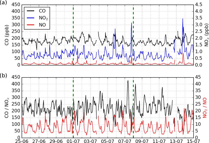
480                                         A. Deroubaix et al.: Diurnal urban pollution transport over southern West Africa

Figure 3. Observed and modeled mean vertical profiles of wind speed (m s−1 ) and direction (360◦ circle with 0 and 360◦ is the north and
90◦ is the east) and relative humidity (RH in %) averaged for all profiles over the period of 1–7 July 2016 at Abidjan in Côte d’Ivoire (green
line), Accra in Ghana (blue line), Cotonou in Benin (purple line), and Savè in Benin (orange line). The mean and standard deviation at the
four locations are represented by the black line and the gray shading. WRF-derived variables are interpolated to the radiosonde positions.
The right panel presents the (mod–obs) mean vertical bias of each location and of the average of the four locations.
Atmos. Chem. Phys., 19, 473–497, 2019                                                        www.atmos-chem-phys.net/19/473/2019/
A. Deroubaix et al.: Diurnal urban pollution transport over southern West Africa                                                          481

Table 4. Observed and modeled distribution (first quartile, median, third quartile), mean and bias (absolute and relative) of relative humidity
(%), and wind direction (◦ ) and speed (m s−1 ) measured by the three aircraft over the period of 1–7 July 2016 separated into three altitude
ranges: surface to 1 km, 1 to 2 km, and 2 to 4 km a.m.s.l.

        Var          N              Q1             Median (Q2)               Q3                Mean                      Bias
                             Obs          Mod       Obs     Mod        Obs         Mod       Obs      Mod     Absolute     Relative (%)
        0 to 1 km
        RH          349    90.75          85.24    94.80    88.65    98.61         93.50    94.19    88.12       −6.07            −6 %
        W. speed    349     3.80           3.98     5.25     5.55     6.47          6.80     5.31     5.51        0.19             4%
        W. dir.     349   220.08         214.17   229.43   228.47   244.41        237.67   231.78   228.19       −3.59            −2 %
        1 to 2 km
        RH          116    91.41          88.10    95.58    90.85    98.77         94.79    94.33    90.86       −3.47           −4 %
        W. speed    116     2.10           1.88     2.90     2.80     4.04          3.94     3.30     3.04       −0.26           −8 %
        W. dir.     116   191.17         207.29   244.71   246.59   285.29        272.28   228.56   228.41       −0.15           > 1%
        2 to 4 km
        RH          62      76.34         73.99    84.43    76.86    90.44         85.18    76.12    79.63        3.51             5%
        W. speed    62       3.34          2.23     4.71     5.69     9.08          9.75     6.37     6.67        0.30             5%
        W. dir.     62      55.73         45.76    72.12    69.04   137.67        145.84   107.36   105.24       −2.12            −2 %

ciated with weak wind speed is a directional shear layer. On              shear layer associated with high RH > 90 % and with low
average, the monsoon layer depth seems to be overestimated                wind speed and changing wind direction; (iii) between 2 and
by about 200 m because the modeled wind direction is biased               4 km a.m.s.l., this is the AEJ layer with RH < 80 %, reversed
by about +20◦ between 1.2 and 2 km a.m.s.l.                               wind direction coming from the northeast, and wind speed
   For the three variables, the profiles of their standard devi-          up to 8 m s−1 . In order to evaluate the model, aircraft mea-
ation present the same modeled and observed characteristics               surements during the daytime are separated into three corre-
(gray shading in Fig. 3). For wind speed, the standard devi-              sponding altitude ranges (Table 4).
ation is about 2 m s−1 from the surface to 2 km a.m.s.l., and                From the surface to 1 km a.m.s.l., the modeled wind speed
it increases up to 4 m s−1 from 2 to 4 km a.m.s.l. For wind               and direction match well with the observations (absolute bias
direction, the standard deviation is low (about 45◦ ) from the            lower than 0.2 m s−1 and 4◦ , respectively). The observed dis-
surface to 1 km a.m.s.l.; it increases from 1 to 2 km in the di-          tribution of the monsoon wind is captured by the model up to
rectional shear layer and it decreases from 2 to 4 km a.m.s.l.            1 km a.m.s.l. (interquartile range 3.80–6.47 m s−1 for the ob-
For RH, the standard deviation is about 10 % from the sur-                servations and 3.98–6.80 m s−1 in the simulation). The mod-
face to 2 km a.m.s.l., and it increases in the AEJ layer but the          eled distribution of RH shows a dry bias in the monsoonal
model does not reproduce the low observed RH values in this               flow (of −6 %).
layer.                                                                       In the directional shear layer, from 1 to 2 km a.m.s.l., ob-
   This analysis shows that the modeled monsoon layer is too              served and modeled wind speed distributions are narrower
deep when it arrives at the coast. Further inland the monsoon             than in the monsoon layer (interquartile ranges being 2.10–
flow is too fast when it reaches Savè. The comparison be-                 4.04 m s−1 and 1.88–3.94 m s−1 , respectively), showing that
tween observed and modeled meteorology also reveals that                  this layer is well defined over the domain. The modeled
the model reproduces the several vertical layers in terms of              wind direction is in good agreement with observations (rel-
wind direction and speed and thus most likely the transport               ative bias lower than 1 %), although with a wider distribu-
that we want to characterize using the tracer experiments well            tion (observed interquartile range 191.17–285.29◦ and mod-
enough.                                                                   eled 214.17–237.67◦ ) than in the monsoon layer (observed
                                                                          interquartile range 220.08–244.41◦ and modeled 207.29–
3.2.2    Identification from research aircraft                            272.28◦ ).
                                                                             In the main easterly layer, from 2 to 4 km a.m.s.l., the ob-
                                                                          served distribution of wind speed is wider at lower altitudes,
The atmospheric vertical structure can be separated into three
                                                                          which is in good agreement with the modeled distribution.
different layers (see Sect. 3.2.1): (i) from the surface to
                                                                          Observed and modeled RH and wind direction distributions
1 km a.m.s.l., there is the monsoon flow with RH > 90 %,
                                                                          are also consistent.
wind speed > 4 m s−1 and direction from the southwesterly
sector; (ii) between 1 and 2 km a.m.s.l., there is a directional

www.atmos-chem-phys.net/19/473/2019/                                                            Atmos. Chem. Phys., 19, 473–497, 2019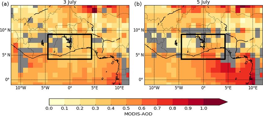
482                                      A. Deroubaix et al.: Diurnal urban pollution transport over southern West Africa

  In conclusion, during the daytime, the monsoon layer is            In contrast to the ATR 42 and Falcon flights, the Twin Ot-
reproduced with a dry bias. The low (relative) biases of wind     ter flew only one time over Savè and made three vertical pro-
speed (+4 %) and direction (−2 %) in this layer are of prime      files up to 3 km a.m.s.l. During the Twin Otter flight in the
importance to accurately model the URB transport.                 afternoon, the range of wind speed increases compared to the
                                                                  two previous flights, reaching between 1 and 12 m s−1 . The
3.3   From the coast to the north: 5 July Lomé–Savè               model reproduces the wind in the monsoon layer well but
      flights                                                     does not capture the wind direction changes between 1 and
                                                                  3 km a.m.s.l. There is no clear change of the direction during
As we want to understand northward pollution transport, we        the first sounding, but during the latter two soundings, wind
need to focus on the wind direction and speed from the coast      direction changes from southwesterly winds at 1 km a.m.s.l.
to the north. In this section, we analyze the spatial vari-       (about 225◦ ) to northeasterly winds at 3 km a.m.s.l. (about
ability in the wind over the Lomé–Savè transect. We com-          45◦ ). The model predicts a too sharp wind direction change
pare aircraft measurements of wind to modeled values us-          from 1 to 3 km a.m.s.l., which shows that the directional
ing data acquired during three specific flights conducted on      shear layer depth is underestimated.
5 July at different times of day with similar flight plans (see      Overall below 1 km a.m.s.l., wind speed ranges from 4
Fig. 1) and similar altitude ranges (i.e., flying mostly below    to 10 m s−1 with a direction from about 250◦ , which is in
2 km a.m.s.l.). The French ATR 42 flight took place between       good agreement with the model. Knippertz et al. (2017) have
08:00 and 11:00 UTC, that of the German Falcon between            shown that 5 July was during a period when the AEJ weak-
11:20 and 15:00 UTC, and that of the British Twin Otter be-       ens and becomes more fragmented, which has led to rela-
tween 16:00 and 17:50 UTC.                                        tively patchy signals in wind and vorticity. This results in
   Using ceilometer measurements, Flamant et al. (2018b)          observed wind direction mostly greater than the third quartile
have described the cloud base height evolution on 5 July at       of the distribution measured over the period of 1–7 July 2016
Savè, which was between 200 and 1000 m during the ATR 42          (Q3 = 244◦ below 1 km a.m.s.l.; see Table 4).
fight, between 400 and 1800 m during the Falcon flight, and          The three aircraft cover the same region from 08:00 to
between 1000 and 3800 m during the Twin Otter flight. This        17:00 UTC. It is thus possible to quantify the evolution of dy-
was a cloudy day, which allowed the operational center to         namical variables during the daytime. We have selected a box
plan for characterizing the diurnal cycle of low level clouds     crossed many times by the aircraft in order to compare hourly
(Flamant et al., 2018b).                                          averages of in situ wind speed and direction observations to
   During the ATR 42 flight in the morning, measurements          the modeled values. The box is delimited in latitude from 6.6
of wind speed range from 2 to 10 m s−1 (Fig. 4). The high-        to 7.8◦ N, in longitude from 1.5 to 2.2◦ E, and in altitude from
est values are observed close to the coast (greater than          300 to 1000 m a.m.s.l. (Fig. A3). When the three flights cross
8 m s−1 ) during the two times the aircraft passes there. The     this box, the average and standard deviation are calculated
model reproduces the spread of the observed values below          from observed values. For the model, we present the average
2 km a.m.s.l. When the altitude reaches 2 km a.m.s.l., ob-        and standard deviation of each hour calculated from all grid
served wind speed decreases below 4 m s−1 . Wind direction        cells included in the box. Wind speed observations decrease
ranges from 240 to 300◦ , even at about 2 km a.m.s.l. The         from 08:00 to 13:00 UTC (Fig. A3), then increase again in
model predicts a constant direction at 250◦ , except when         the afternoon (but there are only a few measurements made
flying above 2 km a.m.s.l. because the modeled direction          by the Twin Otter aircraft in the two boxes at 17:00 UTC).
changes, revealing an underestimation of the modeled PBL          The model does not capture the morning evolution, when the
depth.                                                            NLLJ is eroded, well. We note that the minimum of wind
   In the morning, the monsoon layer is modeled with an           speed is modeled and observed in the early afternoon, when
overestimation of the wind speed and with a sharp directional     vertical mixing is strongest. Observed wind directions are al-
shear at 2 km a.m.s.l., whereas we observe an important vari-     most constant in the box at about 225◦ . There is a change
ability in wind speed without reaching the directional shear      of the direction between 16:00 and 18:00 UTC for both the
layer up to 2 km a.m.s.l. This behavior of the model sug-         model and the observations, which shows the establishment
gests that low-level clouds are not well represented, leading     of the NLLJ.
to modeled PBL depth underestimation.                                On the one hand, these comparisons with aircraft measure-
   During the Falcon flight around midday, wind speed also        ments reinforce our confidence in the model to adequately re-
decreases from the beginning of the flight at the coast (up to    produce the wind speed and direction and thus the main char-
10 m s−1 ) to 100 km further north (less than 4 m s−1 ). Wind     acteristics of pollution transport between Lomé and Savè.
direction varies smoothly from 250◦ at the coast to 300◦ close    On the other hand, this analysis confirms that the PBL depth
to Savè. The model is able to reproduce the weakening of the      is not accurately modeled, especially in the morning, which
monsoon layer linked to daytime dry convection (Adler et al.,     could in turn impact the pollution mixing and dilution. Dur-
2017; Deetz et al., 2018), and the variability in observed and    ing the day, the surface concentration could be overestimated
modeled wind direction and speed is in better agreement.

Atmos. Chem. Phys., 19, 473–497, 2019                                               www.atmos-chem-phys.net/19/473/2019/
A. Deroubaix et al.: Diurnal urban pollution transport over southern West Africa 483 Figure 4. Time series on 5 July 2016 of (a) the French ATR 42, (b) German Falcon, and (c) British Twin Otter aircraft data, composed of three panels for each aircraft: (top) altitude (m) with the latitude (◦ N), (middle) wind speed (m s−1 ), and (bottom) wind direction (degrees). Modeled values with the WRF model are interpolated along the flight positions (red line). Observed value averages are the black dots with the hourly standard deviation (error bars). www.atmos-chem-phys.net/19/473/2019/ Atmos. Chem. Phys., 19, 473–497, 2019
484 A. Deroubaix et al.: Diurnal urban pollution transport over southern West Africa
values noticed in the evening are associated with high NO2
but not with high NO concentrations.
Given the short lifetime of NO (less than 1 h) in the PBL
(Monks et al., 2009), the analysis of NO concentration gives
some clues to understand NO2 variability because NO is
mostly linked to local sources (i.e., not transported). The
baseline of NO concentration is 0.09 ppb (median). High NO
concentrations (> 0.5 ppb) are measured on 1 and 7 July in
the evening. Moreover, there is an increase every evening,
which shows that there are local sources close to the instru-
ment location, probably associated with charcoal stove cook-
ing or traffic time.
In order to identify periods of high NO2 associated with
low NO concentrations, we have computed the NO2 /NO
ratio (Fig. 5b). This ratio is expected to increase at night
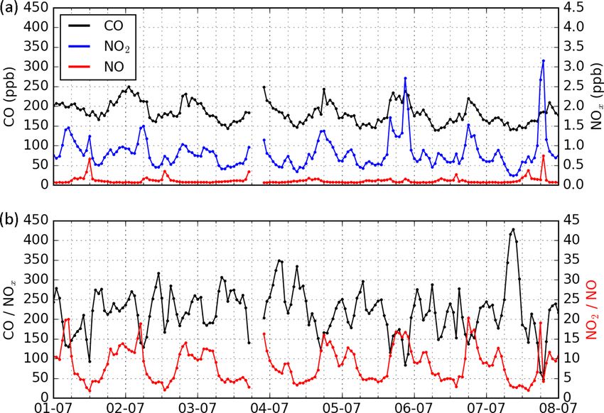
Figure 5. Time series of (a) carbon monoxide (CO), nitrogen diox- by the ozone titration (O3 + NO reaction). During the day-
ide (NO2 ), and nitrogen monoxide (NO) hourly concentration aver- time, it depicts local or transported pollution (respectively a
ages (ppb) observed at Savè (Benin) for the period of 1–7 July 2016
low or high NO2 /NO ratio). Every day we note a sharp in-
and (b) of the ratios CO/NOx (in black) and NO2 /NO (in red). The
crease from 18:00 to 00:00 UTC (NO2 /NO > 15) associated
vertical dashed lines indicate periods of 6 h starting at 00:00 UTC.
with low NO concentrations (NO < 0.2 ppb), which suggests
transported pollutants.
In order to identify periods of high CO associated with
and the concentration at the PBL top height underestimated, low NOx concentrations, we have computed the CO/NOx
especially going further away from the sources. ratio (Fig. 5b). When a BB layer reaches the Guinea coast,
gaseous nitrogen oxide concentrations are lower than 0.1 ppb
(Capes et al., 2009; Reeves et al., 2010) because gaseous ni-
4 Inland pollution transport from the coast trogen oxides have been converted into the particulate phase
during the transport over the southeast Atlantic. We therefore
Firstly, this section investigates CO and NOx concentrations expect an increase in CO and constant NOx , when the BB
at the Savè super-site (Sect. 4.1). Secondly, we analyze the layer reaches Savè without being mixed with URB (contain-
contribution of the major cities along the coastline to the pol- ing NOx in the gaseous phase). At Savè, the CO/NOx ratio
lution budget in Savè (Sect. 4.2). Thirdly, we study how URB is not higher after the arrival of the BB layer on 5 July (see
plumes and the BB layer observed on 5 July interact at the Sect. 3.1). There is an increase in CO together with a NOx
coast and are transported inland. increase; thus when the BB layer reaches Savè, it is mixed
with urban pollution or transported above the PBL.
4.1 Surface pollutant concentrations at Savè In order to determine the diurnal cycle of the three pol-
lutants, we present observed hourly averages over 1–7 July
We analyze the temporal evolution of CO, NO2 , and NO con- together with the maximum and minimum of each hour
centrations. Trace gas concentrations were measured at the measured (Fig. 6). There is a clear diurnal cycle of hourly
ground level at the Savè DACCIWA super-site. We study the CO concentration averages with the minimum occurring at
hourly temporal variability in observed concentrations over 08:00 UTC (about 160 ppb) and with the maximum occurring
the studied period (1 to 7 July). between 18:00 and 22:00 UTC (greater than 200 ppb) over
During this period, the hourly CO concentration varies be- the period of 1–7 July (Fig. 6) and also over the entire cam-
tween 140 and 250 ppb (Fig. 5a). Moreover, looking at the paign period (Fig. A5). This time is in agreement with Adler
entire campaign period (25 June to 15 July), hourly CO con- et al. (2017) and Deetz et al. (2018), who have found us-
centration ranges from 110 to 250 ppb (Fig. A4a). Comparing ing the super-site instrumentation that the coastal front starts
these two periods, we note that our studied period seems rep- moving northward after 16:00 UTC, reaching Savè in the
resentative for the diurnal cycle over the campaign period. evening. It also corresponds to the highest hourly minimum
There is a clear diurnal cycle with the maximum occurring (190 ppb) and maximum (250 ppb). It is worth noting that
every day at the beginning of the night (between 220 and CO concentration remains greater than 180 ppb from 22:00
250 ppb) and the minimum at the beginning of the day. to 04:00 UTC.
Hourly NO2 concentration ranges from 0.2 to 3.5 ppb. We For NO2 , we also note a clear diurnal cycle with low
note also that every day there are periods of high NO2 con- hourly concentration averages between 08:00 and 15:00 UTC
centrations in the evening and low NO2 concentrations from and with high hourly concentration averages (greater than
the morning to the afternoon. It is worth noting that high CO 1 ppb) from 18:00 to 21:00 UTC over the studied period and
Atmos. Chem. Phys., 19, 473–497, 2019 www.atmos-chem-phys.net/19/473/2019/A. Deroubaix et al.: Diurnal urban pollution transport over southern West Africa 485
we analyze Tracer Experiment 1 described in the model sec-
tion (see Table 3 in Sect. 2.3.2).
In order to present this experiment, the synoptic wind pat-
terns and the pollution plumes of the coastal cities with the
URB tracers are displayed in a single figure (Fig. 7). This
figure represents an average of the modeled plumes over
the period of 1–7 July in the monsoon layer (from surface
to 1 km). Results are presented in an arbitrary unit with the
same isocontour value (Iso1) of tracer concentration for each
city (color shadings in Fig. 7).
Over the Gulf of Guinea, we can see markedly higher wind
speed than over the continent. This figure shows that the
pollution plumes of Accra, Lomé, and Cotonou could reach
Savè, while the direction of the Lagos and Abidjan plumes is
not oriented towards Savè.
We now focus on the temporal variability reproduced by
the tracer experiment at Savè (light green dot in Fig. 7). The
Figure 6. Hourly diurnal cycles of (a) carbon monoxide (CO in tracer concentration of the five cities has been interpolated
black), (b) nitrogen dioxide (NO2 in blue), and nitrogen monox-
to Savè coordinates (Fig. 8a). The tracer emissions started
ide (NO in red) concentrations (ppb) observed at Savè (Benin).
Means of each hour are presented by the lines over the period of
on 1 July at 00:00 UTC. The first tracer plume that reaches
1–7 July 2016 and the upper and lower shading limits correspond Savè is that from Cotonou in the evening. We can see that
to the hourly ranges (maximum and minimum of each hour over the tracers emitted from Cotonou reach Savè every day in the
period). evening, typically at around 19:00 UTC. In the morning, the
Lomé pollution plume reaches Savè, while the Accra pollu-
tion plume reaches Savè in the afternoon. There is a short
also over the entire campaign period (Fig. A5). The two small period when hourly concentrations are at a maximum ev-
NO increases (from 0.2 to 0.6 ppb) at 12:00 and 19:00 UTC ery day, and this peak is associated with the arrival of the
are consistent with the usual time of local activities such Cotonou plume in the evening. This pattern is seen repeat-
as traffic and charcoal cooking. At 21:00 UTC, there is a edly over the entire 1–7 July period. The model clearly pre-
high NO2 concentration, as well as a high CO concentration, dicts identified periods when Savè is under the influence of
which is not associated with a high NO concentration, sug- different cities, which implies that these periods correspond
gesting pollution transport because it is the time of the coastal to pollution plumes characterized by different chemical ages.
front passage (Adler et al., 2017; Deetz et al., 2018). From 5 to 6 July, the contribution of Cotonou decreases
The NO2 diurnal cycle is similar to the one of CO with a and the Accra and Lomé contributions increase, which sug-
minimum at 08:00 UTC (about 0.6 ppb) and a maximum be- gests a modification of wind patterns. From midnight to the
tween 18:00 and 21:00 UTC. The main difference of the NO2 end of the night, there is no city plume reaching Savè. How-
and CO diurnal cycles occurs at night between 21:00 and ever, we have seen in Sect. 4.1 that a high CO concentration
02:00 UTC because CO remains high (≈ 200 ppb), whereas persists during the night.
NO2 decreases from 1.3 to 0.7 ppb. This result could be The average diurnal cycle of tracers is presented with the
linked to a higher ratio of BB compared to URB. contribution of each city (Fig. 8b). It confirms that there are
In conclusion, at Savè, there are similar diurnal cycles of distinct periods when Savè is under the successive influences
CO and NO2 with maxima between 18:00 and 21:00 UTC. of Lomé in the morning (06:00 to 12:00 UTC), of Accra in
Moreover NO concentration is very low at 21:00 UTC, indi- the afternoon (12:00 to 18:00 UTC), and of Cotonou in the
cating pollution transport from the coastal urban agglomera- evening (18:00 to 01:00 UTC). Lagos tracers do not reach
tions and not local production. The BB layer could interact Savè because of the southwesterly monsoon flow.
with the URB plumes in the PBL, thus increasing the CO The observed increases in surface concentration may be
concentration. We need to understand how the BB layer is explained by a couple processes: long-range transport of the
mixed with URB at the coast and how it is transported fur- URB plume and/or a local collapse of the nocturnal boundary
ther inland. layer, quickly concentrating locally emitted pollutants. In our
case, the dominant effect is the long-range transport, which is
4.2 Contribution of major coastal cities to the pollution mainly associated with the transport of the Cotonou plume.
budget at Savè Moreover, during the entire campaign, we did not note any
increase in NO at night (Figs. A4 and A5). These results sug-
This section aims at identifying which major cities have a gest that the Cotonou plume affects Savè during a short pe-
significant contribution to inland pollution at Savè. For this, riod with a maximum between 21:00 and 22:00 UTC (about
www.atmos-chem-phys.net/19/473/2019/ Atmos. Chem. Phys., 19, 473–497, 2019You can also read