Automated quantification of floating wood pieces in rivers from video monitoring: a new software tool and validation
←
→
Page content transcription
If your browser does not render page correctly, please read the page content below
Earth Surf. Dynam., 9, 519–537, 2021
https://doi.org/10.5194/esurf-9-519-2021
© Author(s) 2021. This work is distributed under
the Creative Commons Attribution 4.0 License.

             Automated quantification of floating wood pieces
                    in rivers from video monitoring:
                   a new software tool and validation
             Hossein Ghaffarian1 , Pierre Lemaire1,2 , Zhang Zhi1 , Laure Tougne2 , Bruce MacVicar3 , and
                                                    Hervé Piégay1
               1 Univ.Lyon, UMR 5600, Environnement-Ville-Société CNRS, Site EVS, 69362 Lyon, France
                             2 Univ. Lyon, UMR 5205, Laboratoire d’InfoRmatique en Image

                                   et Systèmes d’information CNRS, 69676 Lyon, France
             3 Department of Civil and Environmental Engineering, Univ. Waterloo, Waterloo, Ontario, Canada

                         Correspondence: Hossein Ghaffarian (hossein.ghaffarian@ens-lyon.fr)

                              Received: 9 November 2020 – Discussion started: 20 November 2020
                           Revised: 21 April 2021 – Accepted: 26 April 2021 – Published: 11 June 2021

      Abstract. Wood is an essential component of rivers and plays a significant role in ecology and morphology.
      It can be also considered a risk factor in rivers due to its influence on erosion and flooding. Quantifying and
      characterizing wood fluxes in rivers during floods would improve our understanding of the key processes but are
      hindered by technical challenges. Among various techniques for monitoring wood in rivers, streamside videogra-
      phy is a powerful approach to quantify different characteristics of wood in rivers, but past research has employed
      a manual approach that has many limitations. In this work, we introduce new software for the automatic detec-
      tion of wood pieces in rivers. We apply different image analysis techniques such as static and dynamic masks,
      object tracking, and object characterization to minimize false positive and missed detections. To assess the soft-
      ware performance, results are compared with manual detections of wood from the same videos, which was a
      time-consuming process. Key parameters that affect detection are assessed, including surface reflections, light-
      ing conditions, flow discharge, wood position relative to the camera, and the length of wood pieces. Preliminary
      results had a 36 % rate of false positive detection, primarily due to light reflection and water waves, but post-
      processing reduced this rate to 15 %. The missed detection rate was 71 % of piece numbers in the preliminary
      result, but post-processing reduced this error to only 6.5 % of piece numbers and 13.5 % of volume. The high
      precision of the software shows that it can be used to massively increase the quantity of wood flux data in rivers
      around the world, potentially in real time. The significant impact of post-processing indicates that it is necessary
      to train the software in various situations (location, time span, weather conditions) to ensure reliable results.
      Manual wood detections and annotations for this work took over 150 labor hours. In comparison, the presented
      software coupled with an appropriate post-processing step performed the same task in real time (55 h) on a
      standard desktop computer.

Published by Copernicus Publications on behalf of the European Geosciences Union.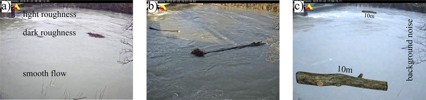
520                   H. Ghaffarian et al.: Automated quantification of floating wood pieces in rivers from video monitoring

1   Introduction                                                   trap most or all of the transported wood, as was observed by
                                                                   Boivin et al. (2015), to quantify wood flux at the flood event
Floating wood has a significant impact on river morphology         or annual scale. All these approaches allow the assessment
(Gurnell et al., 2002; Gregory et al., 2003; Wohl, 2013; Wohl      of the wood budget and in-channel wood exchange between
and Scott, 2017). It is both a component of stream ecosys-         geographical compartments within a given river reach and
tems and a source of risk for human activities (Comiti et al.,     over a given period (Schenk et al., 2014; Boivin et al., 2015,
2006; Badoux et al., 2014; Lucía et al., 2015). The depo-          2017).
sition of wood at given locations can cause a reduction of            For finer-scale information on the transport of wood dur-
the cross-sectional area, which can both increase upstream         ing flood events, video recording of the water surface is suit-
water levels (and the risk for neighboring communities) and        able for estimating instantaneous fluxes and size distribu-
laterally concentrate the flow downstream, which can lead          tions of floating wood in transport (Ghaffarian et al., 2020).
to damaged infrastructure (Lyn et al., 2003; Zevenbergen et        Classic monitoring cameras installed on the riverbank are
al., 2006; Mao and Comiti, 2010; Badoux et al., 2014; Ruiz-        cheap and relatively easy to acquire, set up, and maintain.
Villanueva et al., 2014; De Cicco et al., 2018; Mazzorana et       As is seen in Table 1, a wide range of sampling rates and
al., 2018). Therefore, understanding and monitoring the dy-        spatial–temporal scales have been used to assess wood bud-
namics of wood within a river are fundamental to assess and        gets in rivers. MacVicar and Piégay (2012) and Zhang et
mitigate risk. An important body of work on this topic has         al. (2021) (in review), for instance, monitored wood fluxes
grown over the last 2 decades, which has led to the devel-         at 5 frames per second (fps) and a resolution of 640 × 480
opment of many monitoring techniques (Marcus et al., 2002;         up to 800 × 600 pixels. Boivin et al. (2017) used a simi-
MacVicar et al., 2009a; MacVicar and Piégay, 2012; Benac-          lar camera and frame rate as MacVicar and Piégay (2012)
chio et al., 2015; Ravazzolo et al., 2015; Ruiz-Villanueva et      to compare periods of wood transport with and without the
al., 2019; Ghaffarian et al., 2020; Zhang et al., 2021) and con-   presence of ice. Senter et al. (2017) analyzed the complete
ceptual and quantitative models (Braudrick and Grant, 2000;        daytime record of 39 d of videos recorded at 4 fps and a res-
Martin and Benda, 2001; Abbe and Montgomery, 2003; Gre-            olution of 2048 × 1536 pixels. Conceptually similar to the
gory et al., 2003; Seo and Nakamura, 2009; Seo et al., 2010).      video technique, time-lapse imagery can be substituted for
A recent review by Ruiz-Villanueva et al. (2016), however,         large rivers where surface velocities are low enough and the
argues that the area remains in relative infancy compared to       field of view is large. Kramer and Wohl (2014) and Kramer et
other river processes such as the characterization of channel      al. (2017) applied this technique in the Slave River (Canada)
hydraulics and sediment transport. Many questions remain           and recorded one image every 1 and 10 min. Where pos-
open areas of inquiry including wood hydraulics, which is          sible, wood pieces within the field of view are then visu-
needed to understand wood recruitment, movement and trap-          ally detected and measured using simple software to mea-
ping, and wood budgeting; better parametrization is needed         sure the length and diameter of the wood to estimate wood
to understand and model the transfer of wood in watersheds         flux (pieces per second) or wood volume (m3 s−1 ) (MacVicar
at different scales.                                               and Piégay, 2012; Senter et al., 2017). Critically for this ap-
   In this domain, the quantification of wood mobility and         proach, the time it takes for the researchers to extract in-
wood fluxes in real rivers is a fundamental limitation             formation about wood fluxes has limited the fraction of the
that constrains model development. Most early works were           time that can be reasonably analyzed. Given the outdoor lo-
based on repeated field surveys (Keller and Swanson, 1979;         cation for the camera, the image properties depend heavily on
Lienkaemper and Swanson, 1987), with more recent efforts           lighting conditions (e.g., surface light reflections, low light,
taking advantage of aerial photos or satellite images (Marcus      ice, poor resolution, or surface waves), which may also limit
et al., 2003; Lejot et al., 2007; Lassettre et al., 2008; Senter   the accuracy of frequency and size information (Muste et
and Pasternack, 2011; Boivin et al., 2017) to estimate wood        al., 2008; MacVicar et al., 2009a). In such situations, sim-
delivery at larger timescales of 1 year up to several decades.     pler metrics such as a count of wood pieces, a classification
Others have monitored wood mobility once introduced by             of wood transport intensity, or even just a binary presence–
tracking wood movement in floods (Jacobson et al., 1999;           absence may be used to characterize the wood flux (Boivin
Haga et al., 2002; Warren and Kraft, 2008). Tracking tech-         et al., 2017; Kramer et al., 2017).
nologies such as active and passive radio frequency identi-           A fully automatic wood detection and characterization al-
fication transponders (MacVicar et al., 2009a; Schenk et al.,      gorithm can greatly improve our ability to exploit the vast
2014) or GPS emitters and receivers (Ravazzolo et al., 2015)       amounts of data on wood transport that can be collected from
can improve the precision of this strategy. To better under-       streamside video cameras. From a computer science perspec-
stand wood flux, specific trapping structures such as reser-       tive, however, automatic detection and characterization re-
voirs or hydropower dams can be used to sample the flux            main challenging issues. In computer vision, detecting ob-
over time interval windows (Moulin and Piégay, 2004; Seo           jects within videos typically consists of separating the fore-
et al., 2008; Turowski et al., 2013). Accumulations upstream       ground (the object of interest) from the background (Rous-
of a retention structure can also be monitored where they          sillon et al., 2009; Cerutti et al., 2011, 2013). The basic hy-

Earth Surf. Dynam., 9, 519–537, 2021                                                  https://doi.org/10.5194/esurf-9-519-2021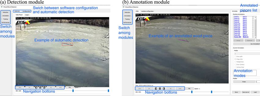
H. Ghaffarian et al.: Automated quantification of floating wood pieces in rivers from video monitoring                                 521

Table 1. Characteristics of streamside video monitoring techniques in different studies.

   Article                         Sampling            Temporal scales                          Camera resolution      Study site
   MacVicar and Piégay (2012)      15 min segments     Three floods, 18 h, 5 fps                640 × 480              Ain, France
   Kramer and Wohl (2014)          Total duration      32 d, 12 761 frames, 0.017 fps           n/a                    Slave, Canada
   Boivin et al. (2017)            Total duration      Three floods, 150 h, 25 fps              640 × 480              St. Jean, Canada
   Kramer et al. (2017)            Total duration      11 months, 0.0017 fps                    1268 × 760             Slave, Canada
   Senter et al. (2017)            15 min segments     39 d, 180 h, 4 fps                       2048 × 1536            North Yuba, USA
   Ghaffarian et al. (2020)        Total duration      Two floods, 80 h, 1 fps                  600 × 800              Isère, France
   Zhang et al. (2021)             Total duration      Seven floods and one windy period,       from 640 × 480 up to   Ain, France
                                                       183 h, 5 fps                             800 × 600

pothesis is that the background is relatively static and covers             approximately 90 % of the wood pieces was detected (i.e.,
a large part of the image, allowing it to be matched between                about 10 % of detections were missed), which confirmed the
successive images. In riverine environments, however, such                  potential utility of this approach. An additional set of false
an assumption is unrealistic because the background shows                   detections related to surface wave conditions amounted to
a flowing river, which can have rapidly fluctuating properties              approximately 15 % of the total detection. However, the de-
(Ali and Tougne, 2009). Floating objects are also partially                 veloped algorithm was not always stable and was found to
submerged in water that has high suspended material con-                    perform poorly when applied to a larger dataset (i.e., video
centrations during floods, making them only partially visible               segments more than 1 h).
(e.g., a single piece of wood may be perceived as multiple                     The objectives of the presented work are to describe and
objects) (MacVicar et al., 2009b). Detecting such an object                 validate a new algorithm and computer interface for quantify-
in motion within a dynamic background is an area of active                  ing floating wood pieces in rivers. First, the algorithm proce-
research (Ali et al., 2012, 2014; Lemaire et al., 2014; Piégay              dure is introduced to show how wood pieces are detected and
et al., 2014; Benacchio et al., 2017). Accurate object detec-               characterized. Second, the computer interface is presented
tion typically relies on the assumption that objects of a single            to show how manual annotation is integrated with the algo-
class (e.g., faces, bicycles, animals) have a distinctive aspect            rithm to train the detection procedure. Third, the procedure
or set of features that can be used to distinguish between                  is validated using data from the Ain River. The validation pe-
types of objects. With the help of a representative dataset,                riod occurred over 6 d in January and December 2012 when
machine-learning algorithms aim to define the most salient                  flow conditions ranged from ∼ 400 m3 s−1 , which is below
visual characteristics of the class of interest (Lemaire et al.,            bankfull discharge but above the wood transport threshold,
2014; Viola and Jones, 2006). When the objects have a wide                  to more than 800 m3 s−1 .
intra-class aspect range, a large amount of data can compen-
sate by allowing the application of deep learning algorithms
(Gordo et al., 2016; Liu et al., 2020). To our knowledge, such              2   Monitoring site and camera settings
a database is not available in the case of floating wood.
   The camera installed on the Ain River in France has been                 The Ain River is a piedmont river with a drainage area of
operating more or less continuously for over 10 years, and                  3630 km2 at the gauging station of Chazey-sur-Ain, with a
vast improvements in data storage mean that these data can                  mean flow width of 65 m, a mean slope of 0.15 %, and a
be saved indefinitely (Zhang et al., 2021). The ability to pro-             mean annual discharge of 120 m3 s−1 . The lower Ain River is
cess this image database to extract the wood fluxes allows us               characterized by an active channel shifting within a forested
to integrate this information over floods, seasons, and years,              floodplain (Lassettre et al., 2008). An AXIS221 Day/Night™
which would allow us to significantly advance our under-                    camera with a resolution of 768 × 576 pixels was installed
standing of the variability within and between floods over a                at this station to continuously record the water surface of
long time period. An unsupervised method to identify float-                 the river at a maximum frequency of 5 fps (Fig. 1). This
ing wood in these videos by applying intensity, gradient, and               camera replaced a lower-resolution camera at the same lo-
temporal masks was developed by Ali and Tougne (2009)                       cation used by MacVicar and Piégay (2012). The specific lo-
and Ali et al. (2011). In this model, the objects were tracked              cation of the camera is on the outer bank of a meander, on
through the frame to ensure that they followed the direction                the side closest to the thalweg, at a height of 9.8 m above
of flow. An analysis of about 35 min of the video showed that               the base flow elevation. The meander and a bridge pier up-
                                                                            stream help to steer most of the floating wood so that it

https://doi.org/10.5194/esurf-9-519-2021                                                         Earth Surf. Dynam., 9, 519–537, 2021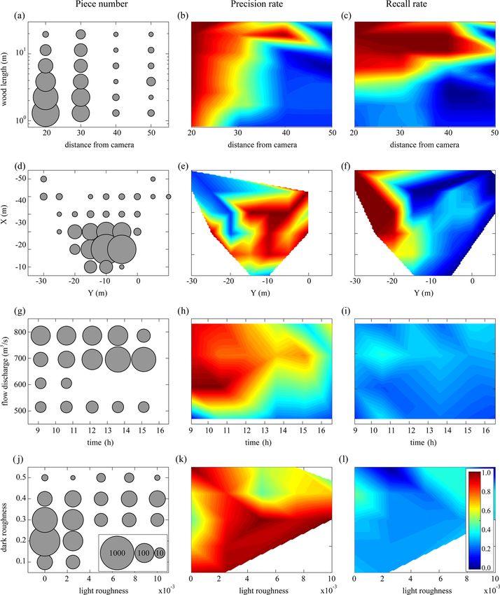
522 H. Ghaffarian et al.: Automated quantification of floating wood pieces in rivers from video monitoring
passes relatively close to the camera where it can be read- area in the upper left. The advantage of this approach is that
ily detected with a manual procedure (MacVicar and Pié- it is computationally very fast. However, misclassification is
gay, 2012). The flow discharge is available from the website possible, particularly when light conditions change.
(http://www.hydro.eaufrance.fr/, last access: 1 June 2020). The second mask, called the dynamic probability mask,
The survey period examined on this river was during 2012, outlines each pixel’s recent history. The corresponding ques-
from which two flood events (1–7 January and 15 December) tion is the following: is this pixel likely to represent wood
were selected for annotation. A range of discharges from 400 now given its past and present characteristics? Again, this
to 800 m3 s−1 occurred during these periods (Fig. 1e), which step is based on what is most common in our database: it
is above a previously observed wood transport threshold of is assumed that a wood pixel is darker than a water pixel.
∼ 300 m3 s−1 (MacVicar and Piégay, 2012). A summary of Depending on lighting conditions like shadows cast on wa-
automated and manual detections for the 6 d is shown in Ta- ter or waves, this is not always true; i.e., water pixels can
ble 3. be as dark as wood pixels. However, pixels displaying suc-
cessively water then wood tend to become immediately and
3 Methodological procedure for automatic detection significantly darker, while pixels displaying wood then water
of wood tend to become significantly lighter. Meanwhile, the intensity
of pixels that keep on displaying wood tends to be rather sta-
The algorithm for wood detection comprises a number of ble. Thus, we assign wood pixel probability according to an
steps that seek to locate objects moving through the field of updated version of the function proposed by Ali et al. (2011)
view in a series of images and then identify the objects most (Fig. 4a) that takes four parameters. This function H is an up-
likely to be wood. The algorithm used in this work modifies dating function, which produces a temporal probability mask
the approach described by Ali et al. (2011). The steps work from the inter-frame pixel value. On a probability map, a
from a pixel to image to video scale, with the context from pixel value ranges from −1 (likely not wood) to 1 (likely
the larger scale helping to assess whether the information at wood). The temporal mask value for a pixel at location (xy)
the smaller scale indicates the presence of floating wood or and at time t is PT (x, y, t) = H (1t , I )+PT (x, y, t − 1). We
not. In a still image, a single pixel is characterized by its loca- apply a threshold to the output of PT (x, y, t) so that it always
tion within the image, its color, and its intensity. Looking at stays within the interval [0, 1]. The idea is that a pixel that be-
its surrounding pixels on an image scale allows information comes suddenly and significantly darker is assumed to likely
to be spatially contextualized. Meanwhile, the video data add be wood. H (1t , I ) is such that under those conditions, it in-
temporal context so that previous and future states of a given creases the pixel probability map value (parameters τ and β).
pixel can be used to assess its likeliness of representing float- A pixel that becomes lighter over time is unlikely to corre-
ing wood. On a video scale, the method can embed expecta- spond to wood (parameter α). A pixel for which the intensity
tions about how wood pieces should move through frames, is stable and that was previously assumed to be wood shall
how big they should be, and how lighting and weather condi- still correspond to wood, while a pixel for which the intensity
tions can evolve to change the expectations of wood appear- is stable and for which the probability to be wood was low
ance, location, and movement. The specific steps followed by is unlikely to represent wood now. A small decay factor (δ)
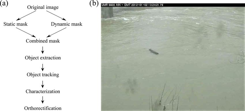
the algorithm are shown in a simple flowchart (Fig. 2a). An was introduced in order to prevent divergence (in particular,
example image with a wood piece in the middle of the frame it prevents noisy areas from being activated too frequently).
is also shown for reference (Fig. 2b). The final wood probability mask is created using a com-
bination of both the static and dynamic probability masks.
Wood objects thus had to have a combination of the cor-
3.1 Wood probability masks
rect pixel color and the expected temporal behavior of water–
In the first step, each pixel was analyzed individually and in- wood–water color. The masks were combined assuming that
dependently. The static probability mask answers the follow- both probabilities are independent, which allowed us to use
ing question: is one pixel likely to belong to a wood block the Bayesian probability rule in which the probability masks
given its color and intensity? The algorithm assumes that the are simply multiplied, pixel by pixel, to obtain the final prob-
wood pixels can be identified by pixel light intensity (i) fol- ability value for each pixel of every frame.
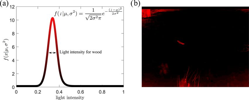
lowing a Gaussian distribution (Fig. 3a). To set the algorithm
parameters, pixel-wise annotations of wood under all the ob- 3.2 Wood object identification and characterization
served lighting conditions were used to determine the mean
(µ) and standard deviation (σ ) of wood piece pixel intensity. From the probability mask it is necessary to group pixels
Applying this algorithm produces a static probability mask with high wood probabilities into objects and then to sepa-
(Fig. 3b). From this figure, it is possible to identify the sec- rate these objects from the background to track them through
tors where wood presence is likely, which includes the float- the image frame. For this purpose, pixels were classified as
ing wood piece seen in Fig. 2b, but also includes standing high or low probability based on a threshold applied to the
vegetation in the lower part of the image and a shadowed combined probability mask. Then, the high-probability pix-
Earth Surf. Dynam., 9, 519–537, 2021 https://doi.org/10.5194/esurf-9-519-2021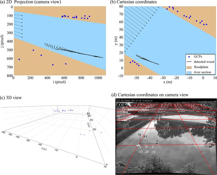
H. Ghaffarian et al.: Automated quantification of floating wood pieces in rivers from video monitoring                                     523

Figure 1. Study site at Pont de Chazey: (a) location of the Ain River catchment in France and location of the gauging station, (b) camera
position and its view angle in yellow, (c) overview of the gauging station with the camera installation point, and (d) view of the river channel
from the camera. (e) Daily mean discharge series for the monitoring period from 1 to 7 January and on 15 December.

Figure 2. (a) Flowchart of the detection software and (b) an example of the frame on which these different flowchart steps are applied.

https://doi.org/10.5194/esurf-9-519-2021                                                          Earth Surf. Dynam., 9, 519–537, 2021
524                     H. Ghaffarian et al.: Automated quantification of floating wood pieces in rivers from video monitoring

Figure 3. Static probability mask, (a) Gaussian distribution of light intensity range for a piece of wood, and (b) employment of a probability
mask on the sample frame.

Figure 4. Dynamic probability mask, (a) updating function H (1t , I ) adapted from Ali et al. (2011), and (b) employment of a probability
mask on the sample frame.

els were grouped into connected components (that is, small,              ject passes between two consecutive frames (Zhang et al.,
contiguous regions on the image) to define the objects. At               2021). Here PT (passing time) is the time that one piece of
this stage, a pixel size threshold was applied to the detected           wood passes through the camera field of view, and 1T is the
objects so that only the bigger objects were considered to               time between two consecutive frames; practically, it is rec-
represent woody objects on the water surface (Fig. 5a the big            ommended to use videos with PT/1T > 5 in this software.
white region in the middle). A number of smaller compo-                  In our case, tracking wood is rather difficult for classical ob-
nents were often related to non-wood objects, for example                ject tracking approaches in computer vision: the background
waves, reflections, or noise from the camera sensor or data              is very noisy, the acquisition frequency is low, and the ob-
compression.                                                             ject’s appearance can be highly variable due to temporarily
   After the size thresholding step, movement direction and              submerged parts and highly variable 3D structures. Given
velocity were used as filters to distinguish real objects from           these considerations it was necessary to use very basic rules
false detections. The question here is the following: is this            for this step. The rules are therefore based on loose expecta-
object moving through the image frame the way we would                   tions, in terms of pixel intervals, regarding the motions of the
expect floating wood to move? To do this, the spatial and                objects depending on the camera location and the river prop-
temporal behavior of components was analyzed. First, to deal             erties. How many pixels is the object likely to move between
with partly immersed objects, we agglomerated multiple ob-               image frames from left to right? How many pixels from top
jects within frames as components of a single object if the              to bottom? How many appearances are required? How many
distance separating them was less than a set threshold. Sec-             frames can we miss because of temporary immersions? Us-
ond, we associated wood objects in successive frames to-                 ing these rules, computational costs remained low and the
gether to determine if the motion of a given object was com-             analysis could be run in real time while also providing good
patible with what is expected from driftwood. This can be                performance.
achieved according to the dimensionless parameter PT/1T ,                   The final step was to characterize each object which at this
which provides a general guideline for the distance an ob-               point in the process are considered wood objects. Each ap-

Earth Surf. Dynam., 9, 519–537, 2021                                                          https://doi.org/10.5194/esurf-9-519-2021
H. Ghaffarian et al.: Automated quantification of floating wood pieces in rivers from video monitoring                                    525

Figure 5. (a) Object extraction by (i) combining static and dynamic masks and (ii) applying a threshold to retain only high-probability pixels.
(b) Object tracking as a filter to deal with partly immersed objects and to distinguish moving objects from static waves.

pears several times in different frames, and a procedure is               metric 2D space thanks to a perspective transform assuming a
needed to either pick a single representative occurrence or               virtual pinhole camera on the image and estimating the posi-
use a statistical tool to analyze multiple occurrences to esti-           tion of the camera and its principal point (center of the view).
mate characterization data. In this step, all images contain-             An example of orthorectification on a detected wood piece in
ing the object are transformed from pixel to Cartesian co-                a set of continuous frames and pixel coordinates (Fig. 6a)
ordinates (as will be described in the next section), and the             is presented in Fig. 6b in metric coordinates. The transform
median length is calculated and used as the most representa-              matrix is obtained with the help of at least four non-colinear
tive state. This approach also matched the manual annotation              points (Fig. 6c, blue GCPs – ground control points – acquired
procedure whereby we tended to pick the view of the object                with DGPS) from which we know both the relative 2D metric
that covers the largest area to make measurements. For the                coordinates for a given water level (Fig. 6b, blue points) and
current paper, every object is characterized from the raw im-             their corresponding localization within the image (Fig. 6a,
age based on its size and its location. It is worth saying that           blue points). To achieve better accuracy, it is advised to ac-
detection was only possible during the daylight.                          quire additional points and to solve the subsequent overde-
                                                                          termined system with the help of a least square regression
3.3   Image rectification                                                 (LSR). Robust estimators such as RANSAC (Forsyth and
                                                                          Ponce, 2012) can be useful tools to prevent acquisition noise.
Warping images according to a perspective transform results               After identifying the virtual camera position, the perspective
in an important loss of quality. On warped images, areas of               transform matrix then becomes parameterized with the water
the image farther from the camera provide little detail and               level. Handling the variable water level was performed for
are overall very blurry and non-informative. Therefore, im-               each piece of wood by measuring the relative height between
age rectification was necessary to calculate wood length, ve-             the camera and the water level at the time of detection based
locity, and volume from the saved pixel-based characteriza-               on information recorded at the gauging station to which the
tion of each object. To do so, the fish-eye lens distortion was           camera was attached. The transformation matrix on the Ain
first corrected. A fish-eye lens distortion is a characteristic           River at the base flow elevation with the camera as the ori-
of the lens that produces visual distortion intended to create            gin is shown in Fig. 6d. Straight lines near the edges of the
a wide panoramic or hemispherical image. This effect was                  image appear curved because the fish-eye distortion has been
corrected by a standard MATLAB process using the Com-                     corrected on this image; conversely, a straight line, in reality,
puterVisionToolbox™ (Release 2017b).                                      is presented without any curvature in the image.
   Ground-based cameras also have an oblique angle of view,
which means that pixel-to-meter correspondence is variable
and images need to be orthorectified to obtain estimates of               4   User interface
object size and velocity in real terms (Muste et al., 2008). Or-
thorectification refers to the process by which image distor-             The software was developed to provide a single environment
tion is removed and the image scale is adjusted to match the              for the analysis of wood pieces on the surface of the water
actual scale of the water surface. Translating from pixels to             from streamside videos. It consists of four distinct modules:
Cartesian coordinates required us to assume that our camera               detection, annotation, training, and performance. The home
follows the pinhole camera model and that the river can be                screen allows the operator to select any of these modules.
assimilated to a plane of constant altitude. Under such con-              From within a module, a menu bar on the left side of the
ditions, it is possible to translate from pixel coordinates to a          interface allows operators to switch from one module to an-

https://doi.org/10.5194/esurf-9-519-2021                                                         Earth Surf. Dynam., 9, 519–537, 2021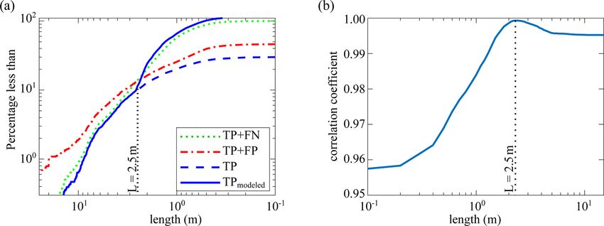
526                     H. Ghaffarian et al.: Automated quantification of floating wood pieces in rivers from video monitoring

Figure 6. Image rectification process. The non-colinear GCPs localization within the image (a) and the relative 2D metric coordinates for a
given water level (b). The different solid lines represent the successive detection in a set of consecutive frames. (c) 3D view of non-colinear
GCPs in metric coordinates. (d) Rectifying transformation matrix on the Ain River at a low flow level with the camera at (0,0,0).

other. In the following sections, the operation of each of these          the output of different masks and the original frames. A con-
modules is described.                                                     figuration tab is available and provides many parameters or-
                                                                          ganized by various categories. The main configuration tab is
                                                                          divided into seven parts. The first part is dedicated to general
4.1   Detection module                                                    configurations such as frames skipped between each compu-
                                                                          tation and defining the areas within the frame where wood
The detection module is the heart of the software. This mod-
                                                                          is not expected (e.g., bridge pier or riverbank). In the second
ule allows, from learned or manually specified parameters,
                                                                          and third parts, the parameters of the intensity and tempo-
the detecting of floating objects without human intervention
                                                                          ral masks are listed (see Sect. 3.1). The default values are
(see Fig. 7). This module contains two main parts: (i) the de-
                                                                          µ = 0.2 and σ = 0.08 for the intensity mask and τ = 0.25
tection tab, which allows the operator to open, analyze and
                                                                          and β = 0.45 for the temporal mask. In the fourth and fifth
export the results from one video or a set of videos; and (ii)
                                                                          parts, object tracking and characterization parameters are re-
the configuration tab, which allows the operator to load and
                                                                          spectively defined as described in Sect. 3.2. Detection time
save the software configuration by defining the parameters of
                                                                          is defined in the sixth part using an optical character recogni-
wood detection (as described in Sect. 3), saving and extract-
                                                                          tion technique. Finally, the parameters of the orthorectifica-
ing the results, and displaying the interface.
                                                                          tion (see Sect. 3.3) are defined in the seventh part. The detec-
   The detection process works as a video file player. The
                                                                          tion software can be used to process videos in batch (“script”
video file (or a stream URL) is loaded to let the software read
                                                                          tab), without generating a visual output, to save computing
the video until the end. When required, the reader generates
                                                                          resources.
a visual output, showing how the masks behave by adding
color and information to the video content (see Fig. 7a). A
small textual display area shows the frequency of past de-                4.2   Annotation module
tections. Meanwhile, the software generates a series of files
summarizing the positive outputs of the detection. They con-              As mentioned in Sect. 2, the detection procedure requires the
sist of YAML and CSV files, as well as image files to show                classification of pixels and objects into wood and non-wood

Earth Surf. Dynam., 9, 519–537, 2021                                                          https://doi.org/10.5194/esurf-9-519-2021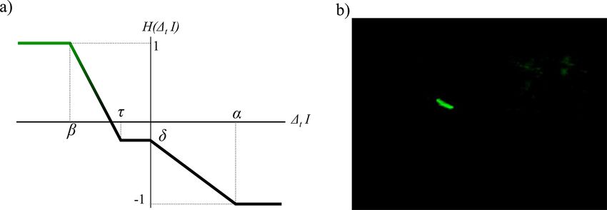
H. Ghaffarian et al.: Automated quantification of floating wood pieces in rivers from video monitoring                             527

Figure 7. User interface of (a) the detection module and (b) the annotation module of the automatic detection software.

categories. To train and validate the automatic detection pro-          scription to each annotation. Each annotation is linked to a
cess, a ground truth or set of videos with manual annotations           single frame of the video; however, a frame can contain sev-
is required. Such annotations can be performed using differ-            eral annotations. An annotated video therefore consists of a
ent techniques. For example, objects can be identified with             video file and a collection of drawings, possibly with textual
the help of a bounding box or selection of end points, as in            descriptions, associated with frames. It is possible to link an-
MacVicar and Piégay (2012), Ghaffarian et al. (2020), and               notations from one frame to another to signify that they be-
Zhang et al. (2021). It is also possible to sample wood pixels          long to the same piece of wood. These data can be used to
without specifying instances or objects and to sample pixels            learn the movement of pieces of wood in the frame.
within annotated objects. Finally, objects and/or pixels can
be annotated multiple times in a video sequence to increase             4.3   Performance module
the amount and detail of information in such an annotation
database. This annotation process is time-consuming, so a               The performance module allows the operator to set rules to
trade-off must be made regarding the purpose of the anno-               compare automatic and manual wood detection results. This
tated database and its required accuracy. Manual annotations            section also allows the operator to use a bare, pixel-based
are especially important when they are intended to be used              annotation or specify an orthorectification matrix to extract
within a training procedure, for which different lighting con-          wood size metrics directly from the output of an automatic
ditions, camera parameters, wood properties, and river hy-              detection.
draulics must be balanced. The rationale for manual annota-                For this module an automatic detection file is first loaded,
tions in the current study is presented in Sect. 5.1.                   and then the result of this detection is compared with a man-
   Given that the tool is meant to be as flexible as possible,          ual annotation for that video if the latter is available. Com-
the annotation module was developed to allow the operator to            parison results are then saved in the form of a summary file
perform annotation in different ways depending on the pur-              (*.csv format), allowing the operator to perform statistical
pose of the study. As shown in Fig. 7.b, this module con-               analysis of the results or the detection algorithm. A manual
tains three main parts: (i) the column on the far left allows           annotation file can only be loaded if it is associated with an
the operator to switch to another module (detection, learn-             automatic detection result.
ing, or performance), (ii) the central part consists of a video            The performance of the detected algorithm can be realized
player with a configuration tab for extracting the data, and            on several levels.
(iii) the right part contains the tools to generate, create, vi-          – Object. The idea is to annotate one (or more) occur-
sualize, and save annotations. The tools allow rather quick                 rence of a single object and to operate the comparison at
coarse annotation, similar to what was done by MacVicar and                 bounding box scale. A detected object may comprehend
Piégay (2012) and Boivin et al. (2015), while still allowing                a whole sequence of occurrences on several frames. It is
the possibility of finer pixel-scale annotation. The principle              validated when only a single occurrence happens to be
of this module is to associate annotations with the frames of               related to an annotation. This is the minimum possible
a given video. Annotating a piece of wood is like drawing                   effort required to have an extensive overview of the ob-
its shape directly on a frame of the video using the drawing                ject frequency on such an annotation database. This ap-
tools provided by the module. It is possible to add a text de-              proach can, however, lead us to misjudge wrongly de-

https://doi.org/10.5194/esurf-9-519-2021                                                      Earth Surf. Dynam., 9, 519–537, 2021
528                    H. Ghaffarian et al.: Automated quantification of floating wood pieces in rivers from video monitoring

       tected sequences as true positives (see below) or vice      Despite overlapping occurrences of wood objects in the two
       versa.                                                      databases, the objects could vary in position and size between
                                                                   them. For the current study we set the TP threshold as the
    – Occurrence. The idea is to annotate, even roughly, every     case in which either at least 50 % of the automatic and an-
      occurrence of every woody object so that the compari-        notated bounding box areas were common or at least 90 %
      son can happen between bounding boxes rather than at         of an automatic bounding box area was part of its annotated
      pixel level. Every occurrence of any detected object can     counterpart.
      be validated individually. This option requires substan-        In addition to the raw counts of TPs, FPs, and FNs, we
      tially more annotation work than the object annotation.      defined two measures of the performances of the application,
    – Pixel. This case implies that every pixel of every oc-       where
      currence of every object is annotated as wood. It is           – recall rate (RR) is the fraction of wood objects automat-
      very powerful in evaluating algorithm performances and           ically detected (TP / (TP + FN)), and
      eventually refining its parameters with the help of some
      machine-learning technique. However, it requires exten-        – precision rate (PR) is the fraction of detected objects
      sive annotation work.                                            that are wood (TP / (TP + FP)).
                                                                   The higher the PR and the RR are, the more accurate our ap-
5     Performance assessment                                       plication is. However, both rates tend to interact. For exam-
                                                                   ple, it is possible to design an application that displays a very
5.1    Assessment procedure
                                                                   high RR (which means that it does not miss many objects)
To assess the performance of the automatic detection algo-         but suffers from a very low PR (it outputs a high amount of
rithm, we used videos from the Ain River in France that were       inaccurate data) and vice versa. Thus, we have to find a bal-
both comprehensively manually annotated and automatically          ance that is appropriate for each application.
analyzed. According to the data annotated by the observer,            It was well known from previous manual efforts to char-
the performance of the software can be affected by different       acterize wood pieces and develop automated detection tools
conditions: (i) wood piece length, (ii) distance from the cam-     that it is easier to detect certain wood objects than others.
era, (iii, iv) wood x and y position, (v) flow discharge, (vi)     In general, the ability to detect wood objects in the dynamic
daylight, and (vii, viii) light and darkness of the frame (see     background of a river in flood was found to vary with the
Table 2). If, for example, software detects a 1 cm piece at a      size of the wood object, its position in the image frame, the
distance of 100 m from the camera, there is a high probabil-       flow discharge, the amount and variability of the light, inter-
ity that this is a false positive detection. Therefore, knowing    ference from other moving objects such as spiders, and other
the performance of the software in different conditions, it is     weather conditions such as wind and rain. In this section, we
possible to develop some rules to enhance the quality of data.     describe and define the metrics that were used to understand
The advantage of this approach is that all eight parameters in-    the variability of the detection algorithm performance.
troduced here are easily accessible in the detection process.         In general, more light results in better detection. The light
In this section the monitoring details and annotation meth-        condition can be changed by varying a set of factors such
ods are introduced before the performance of the software          as weather conditions or the amount of sediment carried by
is evaluated by comparing the manual annotations with the          the river. In any case, the daylight is a factor that can change
automatic detections.                                              the light condition systematically, i.e., low light early in the
   Ghaffarian et al. (2020) and Zhang et al. (2021) show that      morning (Fig. 8a), bright light at midday with the potential
the wood discharge (m3 per time interval) can be measured          for direct light and shadows (Fig. 8b), and low light again in
from the flux or frequency of wood objects (piece number per       the evening, though it is different from the morning because
time interval). An object-level detection was thus sufficient      the hue is more bluish (Fig. 8c). This effect of the time of day
for the larger goals of this research at the Ain River, which is   was quantified simply by noting the time of the image, which
to get a complete budget of transported wood volume.               was marked on the top of each frame of the recorded videos.
   A comparison of annotated with automatic object detec-             Detection is also strongly affected by the frame “rough-
tions gives rise to three options.                                 ness”, defined here as the variation in light over small dis-
                                                                   tances in the frame. The change in light is important for the
    – True positive (TP). An object is correctly detected and is   recognition of wood objects, but light roughness can also oc-
      recorded in both the automatic and annotated database.       cur when there is a region with relatively light pixels due to
    – False positive (FP). An object is incorrectly detected       something such as reflection of the surface of the water, and
      and is recorded only in the automatic database.              dark roughness can occur when there is a region with rel-
                                                                   atively dark pixels due to something such as shadows from
    – False negative (FN). An object is not detected automat-      the surface water waves or surrounding vegetation. Detect-
      ically and is only recorded in the annotated database.       ing wood is typically more difficult around light roughness,

Earth Surf. Dynam., 9, 519–537, 2021                                                  https://doi.org/10.5194/esurf-9-519-2021
H. Ghaffarian et al.: Automated quantification of floating wood pieces in rivers from video monitoring 529
Table 2. Parameters used to assess the performance of the software.
Parameter Rationale Metric
Piece length Larger objects are easier to detect. Detecting an object in pixel coordinates.
Distance Objects closer to the camera are easier to detect. Transferring coordinates to metric.
x position Some particular areas of turbulent flow in the field of Calculating length, position, and distance.
y position view affect detection (e.g., presence of a bridge pier).
Discharge Flow discharge affects water color, turbulence, Recorded water elevation data and calibrated
and the amount of wood. rating curve at hydrologic station.
Time Luminosity of the frames varies with time of day. Time of day as indicated on top of each frame.
Dark roughness Small spots with sharp contrast (either lighter or darker) Percent of pixels below an intensity threshold.
Light roughness affect detection. Percent of pixels above an intensity threshold.
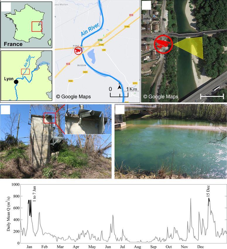
Figure 8. Different light conditions during (a) morning, (b) noon, and (c) late afternoon result in different frame roughnesses and different
detection performances. (c) Wood position can highly affect the quality of detection. Pieces that are passing in front of the camera are detected
much better than the pieces far from the camera.
which results in false negatives, while the color map of a could not be analyzed due to the presence of a spider that
darker surface is often close to that of wood, which results moved around in front of the camera.
in false positives. Both of these conditions can be seen in Flow discharge is another key variable in wood detection.
Fig. 8 (highlighted in Fig. 8a). In general, the frame rough- Increasing flow discharge generally means that water levels
ness increases on windy days or when there is an obstacle are higher, which brings wood close to the near bank of the
in the flow, such as downstream of the bridge pier in the river closer to the camera. This change can make small pieces
current case. The light roughness was calculated for the cur- of wood more visible, but it also reduces the angle between
rent study by defining a light intensity threshold and calculat- the camera position and pixels, which makes wood farther
ing the ratio of pixels of higher value among the frame. The from the camera harder to see. High flows also tend to in-
dark roughness is calculated in the same way, but in this case crease surface waves and velocity, which can increase the
the pixels less than the threshold were counted. In this work roughness of the frame and lead to the wood being intermit-
thresholds equal to 0.9 and 0.4 were used for light and dark tently submerged or obscured. More suspended sediment is
roughness, respectively. carried during high flows, which can change water surface
The oblique view of the camera means that the distance color and increase the opacity of the water.
of the wood piece from the camera is another important fac-
tor in detection (Fig. 8c). The effect of distance on detection
5.2 Detection performance
interacts with wood length; i.e., shorter pieces of wood that
are not detectable near the camera may not be detectable to- Automatic detection software performance was evaluated
ward the far bank due to the pixel size variation (Ghaffarian based on the event based TP, FP, and FN raw numbers as
et al., 2020). Moreover, if a piece of wood passes through a well as the precision (PR) and recall rates (RR) using the
region with high roughness (Fig. 8c) or amongst bushes or default parameters in the software. On average, manual an-
trees (Fig. 8c, right-hand side) it is more likely that the soft- notation resulted in the detection of approximately twice as
ware is unable to detect it. In our case, 1 d of video record many wood pieces as the detection software (Table 3). Mea-
https://doi.org/10.5194/esurf-9-519-2021 Earth Surf. Dynam., 9, 519–537, 2021530 H. Ghaffarian et al.: Automated quantification of floating wood pieces in rivers from video monitoring
sured over all the events, RR = 29 %, which indicates that is fully dependent on piece length so that for lengths of the
many wood objects were not detected by the software, while order of 10 m (L = O(10)) RR is very good. By contrast,
among detected objects about 36 % were false detections when L = O(0.1 ∼ 1), the RR is too small. There is a tran-
(PR = 64 %). sient region when L = O(1), which slightly depends on the
To better understand model performance, we first tested distance from the camera. One can say that the wood length
the correlation between the factors identified in the previ- is the most crucial parameter that affects the recall rate inde-
ous section by calculating each of the eight parameters for pendent of the operator annotation. Based on Fig. 9f, the RR
all detections as one vector and then calculating the corre- is much better on the left side of the frame than on the right
lation between each pair of parameters (Table 4). As shown side. It can be because the operator’s eye needs some time
(the bold values), the pairs of dark–light roughness, length– to detect a piece of wood, so most of the annotations are on
distance, and discharge–time were highly correlated (corre- the right side of the frame. Having a small number of detec-
lations of 0.59, 0.46, and 0.37, respectively). For this reason, tions on the left side of the frame results in the small value
they were considered together to evaluate the performance of FN, which is followed by high values of RR in this region
of the algorithm within a given parameter space. The x/y (RR = TP/(TP+FN). Therefore, while the position of detec-
positions were also considered as a pair despite a relatively tion plays a significant role in the recall rate, it is completely
low correlation (0.15) because they represent the position of dependent on the operator bias. By contrast, frame rough-
an object. As a note, the correlation between time and dark ness, daytime, and flow discharge do not play a significant
roughness is higher than discharge and time, but we used the role in the recall rate (Fig. 9i, l).
discharge–time pair because discharge has a good correla-
tion only with time. As recommended by MacVicar and Pié-
gay (2012), wood lengths were determined on a log-base-2 5.3 Post-processing
transformation to better compare different classes of floating
This section is separated into two main parts. First, we show
wood, similar to what is done for sediment sizes.
how to improve the precision of the software by a posteri-
The presentation of model performance by pairs of cor-
ori distinction between TP and FP. After removing FPs from
related parameters clarifies certain strengths and weaknesses
the detected pieces, in the second part, we test a process to
of the software (Fig. 9). As expected, the results in Fig. 9b
predict the annotated data that the software missed, i.e., false
indicate that, first, the software is not so precise for small
negatives.
pieces of wood (less than the order of 1 m); second, there is
an obvious link between wood length and the distance from
the camera so that by increasing the distance from the cam- 5.3.1 Precision improvement
era, the software is precise only for larger pieces of wood.
Based on Fig. 9e, the software precision is usually better on To improve the precision of the automatic wood detection
the right side of the frame than the left side. This spatial gra- we first ran the software to detect pieces and extracted the
dient in precision is likely because the software requires an eight key parameters for each piece as described in Sect. 5.1.
object to be detected in at least 5 continuous frames for it to Having the value of the eight key parameters (four pairs of
be recognized as a piece of wood (see Sect. 3.2 and Fig. 5 for parameters in Fig. 9) for each piece of wood, we then es-
more information), which means that most of the true posi- timated the total precision of each object, as the average of
tives are on the right side of the frame where five continuous four precisions from each panel in Fig. 9. In the current study
frames have already been established. Also, the presence of the detected piece was considered to be a true positive if the
the bridge pier (at X ∼ = −30 to −40 m based on Fig. 9e) up- total precision exceeded 50 %. To check the validity of this
stream produces lots of waves that decrease the precision of process, we used cross-validation by leaving one day out,
the software. Figure 9h shows that the software is much more calculating the precision matrices based on five other days,
precise during the morning when there is enough light rather and applying the calculated PR matrices on the day that was
than evening when the sunshine decreases. However, at low left out. As is seen in Table 5, this post-processing step in-
flow (Q < 550 m3 s−1 ) the software precision decreases sig- creases the precision of the software to 85 %, which is an en-
nificantly. Finally, based on Fig. 9k, the software does not hancement of 21 %. The degree to which the precision is im-
work well in two roughness conditions: (i) in a dark smooth proved is dependent on the day left out for cross-validation.
flow (light roughness ∼ = 0) when there are some dark patches If, for example, the day left out had similar conditions as the
(shadows) on the surface (dark roughness ∼ = 0.3) and (ii) mean, the PR matrices were well trained and were able to
when roughness increases and there is a lot of noise in a distinguish between TP and FP (e.g., 2 January with 42 %
frame (see Fig. 8). enhancement). On the other hand, if we have an event with
To estimate the fraction of wood pieces that the software new characteristics (e.g., very dark and cloudy weather or at
did not detect, the recall rate (RR) is calculated in different discharges different from what we have in our database), the
conditions, and a linear interpolation was applied to RR as PR matrices were relatively blind and offered little improve-
presented in Fig. 9 (third column). According to Fig. 9c, RR ment (e.g., 15 December with 10 % enhancement).
Earth Surf. Dynam., 9, 519–537, 2021 https://doi.org/10.5194/esurf-9-519-2021H. Ghaffarian et al.: Automated quantification of floating wood pieces in rivers from video monitoring 531
Table 3. Summary of automated and manual detections.
Date Discharge (m3 s−1 ) Water level (m) Detection Number Precision Recall
Qmax Qmin hmax hmin time (h) annot. det. rate % rate %
1 January 2012 718 633 −7.4 −7.8 7 to 17 2282 972 77 33
2 January 2012 772 674 −7.2 −7.6 7 to 17 802 380 52 24
4 January 2012 475 423 −8.4 −8.6 7 to 17 140 158 20 22
6 January 2012 786 763 −7.2 −7.2 7 to 17 712 384 54 29
7 January 2012 462 430 −8.5 −8.6 7 to 17 117 73 40 25
15 December 2012 707 533 −7.5 −8.2 9 to 14 1296 503 72 28
Total 786 423 −7.2 −8.6 55 h 5349 2470 64 29
Table 4. Correlation between parameters. Values in bold show significant correlation.
Dark Light Length Distance x position y position Discharge Time
roughness roughness
Dark roughness 0.59 −0.02 −0.04 0.04 0.1 0 0.57
Light roughness 0.59 −0.03 −0.03 0.03 0.09 −0.04 0.29
Length −0.02 −0.03 0.46 −0.45 −0.35 −0.02 −0.01
Distance −0.04 −0.03 0.46 −1 −0.16 0.14 −0.05
x position 0.04 0.03 −0.45 −1 0.15 −0.15 0.05
y position 0.1 0.09 −0.35 −0.16 0.15 0 0.07
Discharge 0 −0.04 −0.02 0.14 −0.15 0 0.37
Time 0.57 0.29 −0.01 −0.05 0.05 0.07 0.37
One difficulty with the post-processing reclassification of low the threshold, on the other hand, the automatic detec-
wood pieces is that this new step can also introduce error tion software is likely to deviate from the manual counts.
by classifying real objects as false positives (making them a The length distribution obtained from the manual annotations
false negative) or vice versa. Using the training data, we were (TP + FN) (Fig. 10a) was assumed to be the most realistic
able to quantify this error and categorize it as post-processed distribution that can be estimated from the video monitor-
false negatives (FNpp ) with an associated recall rate (RRpp ). ing technique, and it was therefore used as the benchmark.
As shown in Table 5, the precision enhancement process lost Also shown are the raw results of the automatic detection
only around 14 % of TPs (RRpp = 86 %). software (TP + FP) and the raw results with the false posi-
tives removed (TP). At this stage, the difference between the
TP and the TP + FN lines are the false negatives (FN) that
5.3.2 Estimating missed wood pieces based on the
the software has missed. Comparison between the two lines
recall rate
shows that they tend to deviate by 2–3 m. The correlation co-
The automated software detected 29 % of the manually an- efficient between the length distribution of TP as one vector
notated wood pieces (Table 5). In the previous section, meth- and TP + FN as the other vector was calculated for thresh-
ods were described that enhance the precision of the software olds varying from 1 cm to 15 m in length, and 2.5 m was de-
by ensuring that these automatically detected pieces are TPs. fined as the optimum threshold length for recall estimation
The larger question, however, is how to estimate the missing (Fig. 10b).
pieces. Based on Fig. 9, both PR and RR are much higher In the next step we wanted to estimate the pieces less than
for very large objects in most areas of the image and in most 2.5 m that the software missed. During the automatic detec-
lighting conditions. However, the smaller pieces were found tion process, when the software detects a piece of wood, ac-
to be harder to detect, making the wood length the most im- cording to Fig. 9 (third column), the RR can be calculated
portant factor governing the recall rate. Based on this idea, for this piece (same protocol as precision enhancement in
the final step in post-processing is to estimate smaller wood Sect. 5.3.1). Therefore, if, for example, the average recall rate
pieces that were not detected by the software using the length for a piece of wood is 50 %, there is likely to be another piece
distribution extracted by the annotations. in the same condition (defined by the eight different parame-
The estimation is based on the concept of a threshold ters described in Table 2) that the software could not detect.
piece length. Above the threshold, wood pieces are likely To correct for these missed pieces, additional pieces were
to be accurately counted using the automatic software. Be- added to the database; note that these pieces were imaginary
https://doi.org/10.5194/esurf-9-519-2021 Earth Surf. Dynam., 9, 519–537, 2021532 H. Ghaffarian et al.: Automated quantification of floating wood pieces in rivers from video monitoring
Figure 9. Correction matrices: (a, b, c) wood lengths as a function of the distance from the camera, (d, e, f) detection position, (g, h, i)
flow discharges during the daytime, and (j, k, l) light and dark roughnesses. The first column shows the number of all annotated pieces. The
second and third columns show the precision and recall rates of the software, respectively.
pieces inferred from the wood length distribution and were proposed the following equation for calculating wood dis-
not detected by the software. Figure 10a shows the length charge from the wood flux:
distribution after adding these virtual pieces to the database
(blue line, total of 5841 pieces). The result shows good agree- Qw = 0.0086F 1.24 , (1)
ment between this and the operator annotations (green line,
total of 6249 pieces), which results in a relative error of only where Qw is the wood discharge (m3 per 15 min) and F is
6.5 % in the total number of wood pieces. the wood flux (piece number per 15 min). Using this equa-
On the Ain River, by separating videos into 15 min seg- tion, the total volume of wood was calculated based on three
ments, MacVicar and Piégay (2012) and Zhang et al. (2021) different conditions: (i) operator annotation (TP + FN), (ii)
raw data from the detection software (TP + FP), and (iii)
Earth Surf. Dynam., 9, 519–537, 2021 https://doi.org/10.5194/esurf-9-519-2021You can also read