Biogeophysical impacts of forestation in Europe: first results from the LUCAS (Land Use and Climate Across Scales) regional climate model ...
←
→
Page content transcription
If your browser does not render page correctly, please read the page content below
Earth Syst. Dynam., 11, 183–200, 2020
https://doi.org/10.5194/esd-11-183-2020
© Author(s) 2020. This work is distributed under
the Creative Commons Attribution 4.0 License.

          Biogeophysical impacts of forestation in Europe: first
         results from the LUCAS (Land Use and Climate Across
             Scales) regional climate model intercomparison
      Edouard L. Davin1 , Diana Rechid2 , Marcus Breil3 , Rita M. Cardoso4 , Erika Coppola5 , Peter Hoffmann2 ,
          Lisa L. Jach6 , Eleni Katragkou7 , Nathalie de Noblet-Ducoudré8 , Kai Radtke9 , Mario Raffa10 ,
        Pedro M. M. Soares4 , Giannis Sofiadis7 , Susanna Strada5 , Gustav Strandberg11 , Merja H. Tölle12 ,
                                 Kirsten Warrach-Sagi6 , and Volker Wulfmeyer6
                    1 Department        of Environmental Systems Science, ETH Zurich, Zurich, Switzerland
            2 Climate       Service Center Germany (GERICS), Helmholtz-Zentrum Geesthacht, Hamburg, Germany
           3 Institute of Meteorology and Climate Research, Karlsruhe Institute of Technology, Karlsruhe, Germany
            4 Instituto Dom Luiz (IDL), Faculdade de Ciências, Universidade de Lisboa, 1749-016 Lisboa, Portugal
                5 International Center for Theoretical Physics (ICTP), Earth System Physics Section, Trieste, Italy
                        6 Institute of Physics and Meteorology, University of Hohenheim, Stuttgart, Germany
                      7 Department of Meteorology and Climatology, School of Geology, Aristotle University

                                                 of Thessaloniki, Thessaloniki, Greece
               8 Laboratoire des Sciences du Climat et de l’Environnement; UMR CEA-CNRS-UVSQ, Université

                           Paris-Saclay, Orme des Merisiers, bât 714, 91191 Gif-sur-Yvette CÉDEX, France
       9 Chair of Environmental meteorology, Brandenburg University of Technology, Cottbus-Senftenberg, Germany
                10 REgional Models and geo-Hydrological Impacts, Centro Euro-Mediterraneo sui Cambiamenti

                                                        Climatici, Lecce, Italy
                         11 Swedish Meteorological and Hydrological Institute and Bolin Centre for Climate

                                                    Research, Norrköping, Sweden
         12 Department of Geography, Climatology, Climate Dynamics and Climate Change, Justus Liebig University

                                                      Gießen, Gießen, Germany
                            Correspondence: Edouard L. Davin (edouard.davin@env.ethz.ch)

                                 Received: 31 January 2019 – Discussion started: 8 February 2019
                     Revised: 29 November 2019 – Accepted: 4 December 2019 – Published: 20 February 2020

      Abstract. The Land Use and Climate Across Scales Flagship Pilot Study (LUCAS FPS) is a coordinated com-
      munity effort to improve the integration of land use change (LUC) in regional climate models (RCMs) and to
      quantify the biogeophysical effects of LUC on local to regional climate in Europe. In the first phase of LUCAS,
      nine RCMs are used to explore the biogeophysical impacts of re-/afforestation over Europe: two idealized ex-
      periments representing respectively a non-forested and a maximally forested Europe are compared in order to
      quantify spatial and temporal variations in the regional climate sensitivity to forestation. We find some robust
      features in the simulated response to forestation. In particular, all models indicate a year-round decrease in sur-
      face albedo, which is most pronounced in winter and spring at high latitudes. This results in a winter warming
      effect, with values ranging from + 0.2 to +1 K on average over Scandinavia depending on models. However,
      there are also a number of strongly diverging responses. For instance, there is no agreement on the sign of tem-
      perature changes in summer with some RCMs predicting a widespread cooling from forestation (well below
      −2 K in most regions), a widespread warming (around +2 K or above in most regions) or a mixed response.
      A large part of the inter-model spread is attributed to the representation of land processes. In particular, dif-
      ferences in the partitioning of sensible and latent heat are identified as a key source of uncertainty in summer.
      Atmospheric processes, such as changes in incoming radiation due to cloud cover feedbacks, also influence the

Published by Copernicus Publications on behalf of the European Geosciences Union.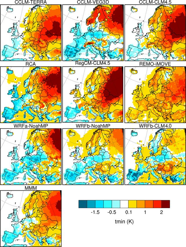
184                                                           E. L. Davin et al.: Biogeophysical impacts of forestation in Europe

       simulated response in most seasons. In conclusion, the multi-model approach we use here has the potential to
       deliver more robust and reliable information to stakeholders involved in land use planning, as compared to results
       based on single models. However, given the contradictory responses identified, our results also show that there
       are still fundamental uncertainties that need to be tackled to better anticipate the possible intended or unintended
       consequences of LUC on regional climates.

1   Introduction                                                     and considering timescales from extreme events to seasonal
                                                                     and multi-decadal trends and variability. LUCAS is designed
Land use change (LUC) affects climate through biogeophys-            in successive phases that will go from idealized to realis-
ical processes influencing surface albedo, evapotranspiration        tic high-resolution scenarios and intends to cover both land
and surface roughness (Bonan, 2008; Davin and de Noblet-             cover changes and land management impacts.
Ducoudré, 2010). The quantification of these effects is still           In the first phase of LUCAS, which is the focus of this
subject to particularly large uncertainties, but there is grow-      study, idealized experiments over Europe are performed in
ing evidence that LUC is an important driver of climate              order to benchmark the RCM sensitivity to extreme LUC.
change at local to regional scales. For instance, the Land-          Two experiments (FOREST and GRASS) are performed us-
Use and Climate, IDentification of robust impacts (LUCID)            ing a set of nine RCMs. The FOREST experiment represents
model intercomparison indicated that while LUC likely had            a maximally forested Europe, while in the GRASS experi-
a modest biogeophysical impact on global temperature since           ment trees are replaced by grassland. Comparing FOREST
the pre-industrial era, it may have affected temperature in a        to GRASS therefore indicates the theoretical potential of a
similar proportion to greenhouse gas forcing in some regions         maximum-forestation (encompassing both reforestation and
(de Noblet-Ducoudré et al., 2012). Results from the Coupled          afforestation) scenario over Europe. Given that forestation is
Model Intercomparison Project Phase 5 (CMIP5) confirmed              one of the most prominent land-based mitigation strategies
the importance of LUC for regional climate trends and for            put forward in scenarios compatible with the Paris Agree-
temperature extremes (Kumar et al., 2013; Lejeune et al.,            ment goals (Grassi et al., 2017; Griscom et al., 2017; Harper
2017, 2018).                                                         et al., 2018), it is essential to understand its full consequences
   In this light, it is particularly important to represent LUC      beyond CO2 mitigation. These experiments are not meant
forcings not only in global climate models but also in re-           to represent realistic scenarios, but they enable a system-
gional climate simulations. Yet, LUC forcings were not in-           atic assessment and mapping of the biogeophysical impact
cluded in previous regional climate model (RCM) intercom-            of forestation across regions and seasons. Experiments of
parisons (Christensen and Christensen, 2007; Jacob et al.,           this type have already been performed using single regional
2014; Mearns et al., 2012; Solman et al., 2013), which are           or global climate models (Cherubini et al., 2018; Claussen
the basis for numerous regional climate change assessments           et al., 2001; Davin and de Noblet-Ducoudré, 2010; Strand-
providing information for impact studies and the design of           berg et al., 2018), but here they are performed for the first
adaptation plans (Gutowski Jr. et al., 2016). RCMs have been         time using a multi-model ensemble approach, thus providing
applied individually to explore different aspects of land use        an unprecedented opportunity to assess uncertainties in the
impacts on regional climates (Davin et al., 2014; Gálos et al.,      climate response to vegetation perturbations. In the follow-
2013; Lejeune et al., 2015; Tölle et al., 2018; Wulfmeyer et         ing, we focus on the analysis of the surface energy balance
al., 2014), but the robustness of such results is difficult to as-   and temperature response at the seasonal timescale, while fu-
sess due to their reliance on single RCMs and due to the lack        ture studies within LUCAS will explore further aspects (sub-
of a common protocol. There is therefore a need for a coor-          daily timescale and extreme events, land–atmosphere cou-
dinated effort to better integrate LUC effects in RCM pro-           pling, etc.). We aim to quantify the potential effect of foresta-
jections. The Land Use and Climate Across Scales (LUCAS)             tion over Europe, identify robust model responses, and in-
initiative (https://www.hzg.de/ms/cordex_fps_lucas/, last ac-        vestigate the possible sources of uncertainty in the simulated
cess: 10 February 2020) has been designed with this goal in          impacts.
mind. LUCAS is endorsed as a Flagship Pilot Study (FPS) by
the World Climate Research Program-Coordinated Regional              2     Methods
Climate Downscaling Experiment (WCRP-CORDEX) and
was initiated by the European branch of CORDEX (EURO-                2.1    RCM ensemble
CORDEX) (Rechid et al., 2017). The objectives of the LU-
CAS FPS are to promote the inclusion of the missing LUC              Two experiments (GRASS and FOREST) were performed
forcing in RCM multi-model experiments and to identify the           with an ensemble of nine RCMs, whose names and char-
associated impacts with a focus on regional to local scales          acteristics are presented in Table 1. All experiments were

Earth Syst. Dynam., 11, 183–200, 2020                                                   www.earth-syst-dynam.net/11/183/2020/
E. L. Davin et al.: Biogeophysical impacts of forestation in Europe                                                             185

performed at 0.44◦ (∼ 50 km) horizontal resolution on the               The starting point for both maps is a MODIS-based
EURO-CORDEX domain (Jacob et al., 2014) with lateral                 present-day land cover map at 0.5◦ resolution (Lawrence and
boundary conditions and sea surface temperatures prescribed          Chase, 2007) providing the global distribution of 17 plant
based on 6-hourly ERA-Interim reanalysis (Dee et al., 2011).         functional types (PFTs). Crops and shrubs which are present
The simulations are analysed over the period 1986–2015, and          in the original map are not considered in the FOREST and
the earlier years (1979–1985 or a subset of these years de-          GRASS experiments and are set to zero. To create the FOR-
pending on models; see Table 1) were used as spin-up period.         EST map, the fractional coverage of trees is expanded until
The model outputs were aggregated to monthly values for use          trees occupy 100 % of the non-bare soil area. The proportion
in this study. When showing results averaged across all nine         of various tree types (i.e. broadleaf to needleleaf and decidu-
RCMs, we refer to it as the multi-model mean (MMM).                  ous to evergreen) is conserved as in the original map as well
   A notable characteristic of the multi-model ensemble is           as the fractional coverage of bare soil, which prevents ex-
that some RCMs share the same atmospheric scheme (i.e.               panding vegetation on land areas where it could not realisti-
same version and configuration) but are coupled to different         cally grow (e.g. in deserts). If no trees are present in a given
land surface models (LSMs) or share the same LSM in com-             grid cell with less than 100 % bare soil, the zonal mean forest
bination with different atmospheric schemes (see Table 1).           composition is taken as a representative value. This results in
This allows us to evaluate the respective influence of atmo-         a map with only tree PFTs (PFT names) and bare soil, all
spheric versus land process representation. For instance, the        other vegetation types being shrunk to zero. It is important
same version of COSMO-CLM (CCLM) is used in com-                     to note that this FOREST map does not represent a poten-
bination with three different LSMs (TERRA_ML, VEG3D                  tial vegetation map, which would imply a more conservative
and CLM4.5). Comparing results from these three CCLM-                assumption in terms of forest expansion potential. Indeed,
based configurations enables us to isolate the role of land          trees can grow even in regions where they would not natu-
process representation in this particular model. Conversely,         rally occur because of various human interventions (assisted
CLM4.5 is used in combination with two different RCMs                afforestation, forest management, fire suppression, etc.). This
(CCLM and RegCM), which allows us to diagnose the in-                FOREST map is therefore in line with the idea of consider-
fluence of atmospheric processes on the results. Different           ing both reforestation and afforestation potential, while still
configurations of WRF (Weather Research and Forecasting)             excluding forest expansion over dryland regions where irri-
are also used: WRFa-NoahMP and WRFb-NoahMP differ                    gation measures would likely be necessary.
only in their atmospheric set-up, while WRFb-NoahMP and                 The GRASS map is then derived from the FOREST map
WRFb-CLM4.0 share the same atmospheric set-up but with               by converting all tree PFTs into grassland PFTs, the C3 -to-C4
different LSMs.                                                      ratio being conserved as in the original MODIS-based map
   While the simulations we present are not suitable for             as well as the bare soil fraction.
model evaluation because of the idealized land cover char-              Since the various RCMs use different land use classifi-
acteristics, it is worthwhile to note that the RCMs included         cation schemes (see Table 1), the PFT-based FOREST and
here have been part of previous evaluation studies over Eu-          GRASS maps were converted into model-specific land use
rope (e.g. Kotlarski et al., 2014; Davin et al., 2016). Although     classes for implementation into the respective RCMs. The
for a given RCM the model version and configuration may              specific conversion rules used in each RCM are summarized
differ from previously evaluated configurations, the system-         in Table 1 (note that for three out of the nine RCMs, no con-
atic biases highlighted in these previous studies are likely still   version was required). Urban areas, inland water and glacier,
relevant here. In particular, a majority of RCMs suffer from         if included in a given RCM, were conserved as in the stan-
predominantly cold and wet biases in most European regions,          dard dataset of the respective RCM.
while the opposite is true in summer in Mediterranean re-
gions (Kotlarski et al., 2014). The conditions that are too dry
                                                                     3     Results
over southern Europe have been related in particular to land
surface process representation including evapotranspiration          3.1    Temperature response
(Davin et al., 2016).
                                                                     The effect of forestation (FOREST minus GRASS) on sea-
                                                                     sonal mean winter 2 m temperature is shown in Fig. 1. All
2.2   FOREST and GRASS vegetation maps                               RCMs simulate a warming pattern which is strongest in
                                                                     the northeast of Europe. This warming effect weakens to-
Two vegetation maps have been created for use in the Phase           ward the southwest of the domain even changing sign for in-
1 LUCAS experiments (Fig. S1 in the Supplement). The veg-            stance in the Iberian Peninsula (except for REMO-iMOVE).
etation map used in the experiment FOREST is meant to rep-           In summer (Fig. 2), there is a very large spread of model re-
resent a theoretical maximum of tree coverage, while in the          sponses with some RCMs predicting a widespread cooling
vegetation map used in the experiment GRASS, trees are en-           from forestation (CCLM-TERRA and RCA), a widespread
tirely replaced by grassland.                                        warming (RegCM-CLM4.5, REMO-iMOVE and the WRF

www.earth-syst-dynam.net/11/183/2020/                                                   Earth Syst. Dynam., 11, 183–200, 2020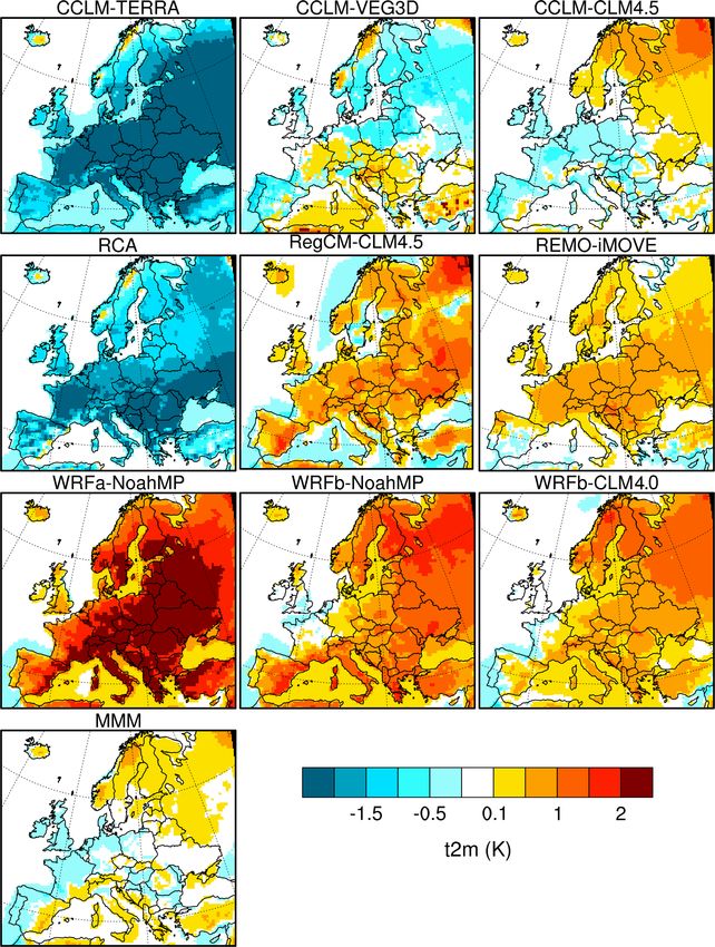
E. L. Davin et al.: Biogeophysical impacts of forestation in Europe
www.earth-syst-dynam.net/11/183/2020/
Table 1. Names and characteristics of the RCMs used. NET-Temperate: needleleaf evergreen tree – temperate; NET-Boreal: needleleaf evergreen tree – boreal; NDT-Boreal: needleleaf
deciduous tree – boreal; BET-Tropical: broadleaf evergreen tree – tropical; BET-Temperate: broadleaf evergreen tree – temperate; BDT-Tropical: broadleaf deciduous tree – tropical;
BDT-Temperate: broadleaf deciduous tree – temperate; BDT-Boreal: broadleaf deciduous tree – boreal; BES-Temperate: broadleaf evergreen shrub – temperate; BDS-Temperate:
broadleaf deciduous shrub – temperate; BDS-Boreal: broadleaf deciduous shrub – boreal. Institution IDs are as follows: JLU – Justus-Liebig-Universität Gießen; BTU: Brandenburgische
Technische Universität; KIT – Karlsruhe Institute of Technology; ETH – Eidgenössische Technische Hochschule Zürich; SMHI – Swedish Meteorological and Hydrological Institute;
ICTP – International Centre for Theoretical Physics; GERICS – Climate Service Center Germany; IDL – Instituto Amaro Da Costa; UHOH – University of Hohenheim; AUTH –
Aristotle University of Thessaloniki.
Model name CCLM-TERRA CCLM-VEG3D CCLM-CLM4.5 RCA RegCM-CLM4.5 REMO-iMOVE WRFa-NoahMP WRFb-NoahMP WRFb-CLM4.0
Institute ID JLU/BTU/CMCC KIT ETH SMHI ICTP GERICS IDL UHOH AUTH
RCM COSMO_5.0_clm9 COSMO_5.0_clm9 COSMO_5.0_clm9 RCA4 RegCM4.6.1 REMO2009 WRF381 WRF381 WRF381
(Giorgi et al., 2012)
Land settings
Land surface scheme TERRA-ML (Schrodin and VEG3D (Breil et CLM4.5 (Oleson et (Samuelsson et al., CLM4.5 (Oleson et iMOVE (Wilhelm NoahMP NoahMP CLM4.0 (Oleson et
Heise, 2001) al., 2018) al., 2013) 2006) al., 2013) et al., 2014) al., 2010)
Land cover classes (classes ef- 1: BET 1: bare soil 1: bare soil 1: bare soil 1: bare soil 1: tr. br. everg. 1: NET 1: NET 1: NET
fectively used in FOREST and 2: BDT closed 2: water 2: NET- 2: open land 2: NET- 2: tr. br. decidu- 2: NDT 2: NDT 2: NDT
GRASS in bold) 3: BDT open 3: urban Temperate 3: needleleaf for- Temperate ous 3: BET 3: BET 3: BET
4: NET 4: deciduous for- 3: NET-Boreal est 3: NET-Boreal 3: temp. br. everg. 4: BDT 4: BDT 4: BDT
5: NDT est 4: NDT-Boreal 4: broadleaf forest 4: NDT-Boreal 4: temp. br. decid- 5: mixed forests 5: mixed forests 5: mixed forests
6: mixed leaf trees 5: coniferous for- 5: BET-Tropical 5: BET-Tropical uous 6: closed shrubland 6: closed shrubland 6: closed shrubland
7: fresh water flooded trees est 6: BET- 6: BET- 5: everg. conif. 7: open shrubland 7: open shrubland 7: open shrubland
8: saline water flooded trees 6: mixed forest Temperate Temperate 6: deciduous 8: wooded savan- 8: wooded savan- 8: wooded savan-
9: mosaic tree/natural veget. 7: cropland 7: BDT-Tropical 7: BDT-Tropical conif. nah nah nah
10: burnt tree cover 8: special crops 8: BDT- 8: BDT- 7: everg. shrubs 9: savannah 9: savannah 9: savannah
11: everg. shrubs closed/open 9: grassland Temperate Temperate 8: deciduous 10: grassland 10: grassland 10: grassland
12: deciduous shrubs 10: shrubland 9: BDT-Boreal 9: BDT-Boreal shrubs 11: wetlands 11: wetlands 11: wetlands
closed/open 10: BDS- 10: BDS- 9: C3 grasses 12: cropland 12: cropland 12: cropland
13: herbac. veget. closed/open Temperate Temperate 10: C4 grasses 13: urban and 13: urban and 13: urban and
14: grass 11: BES- 11: BES- 11: tundra built-up built-up built-up
15: flooded shrubs or herbac. Temperate Temperate 12: swamps 14: crop- 14: crop- 14: crop-
16: cultivated and managed 12: BDS-Boreal 12: BDS-Boreal 13: C3 crops land/natural land/natural land/natural
17: mosaic crop/tree/net veget. 13: C3 arctic 13: C3 arctic 14: C4 crops vegetation mosaic vegetation mosaic vegetation mosaic
18: mosaic crop/shrub/grass grass grass 15: urban 15: snow and ice 15: snow and ice 15: snow and ice
19: bare areas 14: C3 grass 14: C3 grass 16: bare 16: barren or 16: barren or 16: barren or
20: water 15: C4 grass 15: C4 grass sparsely sparsely sparsely
21: snow and ice 16: crop 1 16: crop 1 vegetated vegetated vegetated
Earth Syst. Dynam., 11, 183–200, 2020
22. artificial surface 17: crop 2 17: crop 2 17: water 17: water 17: water
23: undefined 18: wooded tundra 18: wooded tundra 18: wooded tundra
19: mixed tundra 19: mixed tundra 19: mixed tundra
20: barren tundra 20: barren tundra 20: barren tundra
21: lakes 21: lakes 21: lakes
Conversion method to imple- bare soil = 19 bare soil = 1 no conversion bare soil = 1 no conversion bare soil = 16 bare soil = 16 bare soil = 16 bare soil = 16
ment the PFT-based input veg- NET-Temperate = 4 NET-Temperate = needed NET-Temperate = needed NET-Temperate = NET-Temperate = NET-Temperate = NET-Temperate =
etation maps (FOREST and NET-Boreal = 4 5 3 5 1 1 1
GRASS) NDT-Boreal = 5 NET-Boreal = 5 NET-Boreal = 3 NET-Boreal = 5 NET-Boreal = 1 NET-Boreal = 1 NET-Boreal = 1
BET-Temperate = 1 NDT-Boreal = 5 NDT-Boreal = 3 NDT-Boreal = 6 NDT-Boreal = 2 NDT-Boreal = 2 NDT-Boreal = 2
BDT-Temperate = 2 BET-Temperate = BET-Temperate = BET-Temperate = BET-Temperate = BET-Temperate = BET-Temperate =
BDT-Boreal = 3 4 4 3 3 3 3
C3 arctic BDT-Temperate = BDT-Temperate = BDT-Temperate = BDT-Temperate = BDT-Temperate = BDT-Temperate =
grass = 14 4 4 4 4 4 4
C3 grass = 14 BDT-Boreal = 4 BDT-Boreal = 4 BDT-Boreal = 4 BDT-Boreal = 4 BDT-Boreal = 4 BDT-Boreal = 4
C4 grass = 14 C3 arctic C3 arctic grass = 2 C3 arctic grass = 9 C3 arctic C3 arctic C3 arctic
grass = 9 C3 grass = 2 C3 grass = 9 grass = 10 grass = 10 grass = 10
C3 grass = 9 C4 grass = 2 C4 grass = 10 C3 grass = 10 C3 grass = 10 C3 grass = 10
C4 grass = 9 C4 grass = 10 C4 grass = 10 C4 grass = 10
186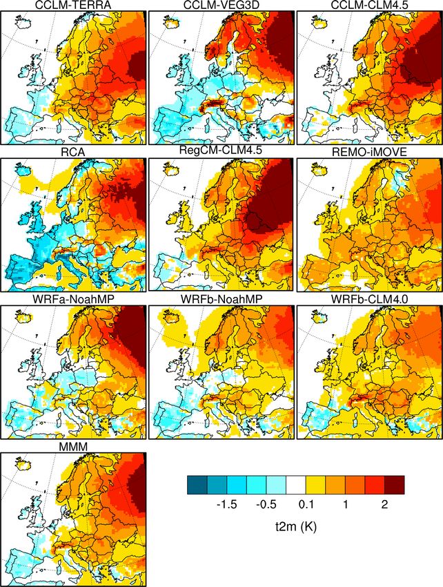
Table 1. Continued.
Model name CCLM-TERRA CCLM-VEG3D CCLM-CLM4.5 RCA RegCM-CLM4.5 REMO-iMOVE WRFa-NoahMP WRFb-NoahMP WRFb-CLM4.0
Institute ID JLU/BTU/CMCC KIT ETH SMHI ICTP GERICS IDL UHOH AUTH
RCM COSMO_5.0_clm9 COSMO_5.0_clm9 COSMO_5.0_clm9 RCA4 RegCM4.6.1 REMO2009 WRF381 WRF381 WRF381
(Giorgi et al., 2012)
Land settings
Representation of sub-grid- single class single class tile approach tile approach tile approach tile approach single class single class tile approach
scale vegetation heterogeneity
Leaf area index prescribed seasonal cycle (sinus prescribed seasonal prescribed seasonal Calculated monthly prescribed seasonal Calculated daily prescribed seasonal prescribed seasonal prescribed seasonal
function depending on altitude cycle (sinus func- cycle based on based on vegetation cycle based on based on atmo- cycle based on cycle based on cycle based on
and latitude with vegetation- tion depending on MODIS (Lawrence type, soil tempera- MODIS (Lawrence spheric forcing and lookup tables lookup tables MODIS (Lawrence
dependent minimum and max- altitude and latitude and Chase, 2007) ture and soil mois- and Chase, 2007) soil moisture state and Chase, 2007)
imum values) with vegetation- ture
dependent mini-
mum and maxi-
mum values)
www.earth-syst-dynam.net/11/183/2020/
Total soil depth and number of nine thermally active layers nine layers down to 15 layers for ther- five layers down to 15 layers for ther- five thermally four layers down to four layers down to 10 layers down to
hydrologically/thermally active down to 7.5 m; first eight hydro- 7.5 m mal calculations 2.89 m mal calculations active layers down 1m 1m 3.43 m
soil layers logically active down to 3.9 m down to 42 m; first down to 42 m; first to 10 m; one water
10 hydrologically 10 hydrologically bucket
active down to active down to
3.43 m 3.43 m
Atmospheric settings
Initialization and spin-up Initialization with ERA- Initialization with Initialization with Initialization with Initialization with Initialization with Initialization with Initialization with Initialization with
Interim, 1979–1985 as spin-up ERA-Interim, ERA-Interim, ERA-Interim, ERA-Interim ex- ERA-Interim, ERA-Interim, ERA-Interim, ERA-Interim,
1979–1985 as 1979–1985 as 1979–1985 as cept soil moisture, 1979–1985 as 1979–1985 as 1983–1985 as 1984–1985 as
spin-up spin-up spin-up which is based on spin-up spin-up spin-up spin-up
a climatological
E. L. Davin et al.: Biogeophysical impacts of forestation in Europe
average (Giorgi et
al., 1989); 1985 as
spin-up
Lateral boundary formulation Davies (1976) Davies (1976) Davies (1976) Davies (1976) with Giorgi et al. (1993) Davies (1976) exponential relax- exponential relax- exponential relax-
a cosine-based re- ation ation ation
laxation function
Buffer (no. of grid cells) 13 13 13 8 12 8 15 10 10
No. of vertical levels 40 40 40 24 23 27 50 40 40
Turbulence and planetary Level 2.5 closure for turbu- Level 2.5 closure Level 2.5 closure (Vogelezang and The University of Vertical diffusion MYNN (Mellor– MYNN Level 2.5 MYNN Level 2.5
boundary layer scheme lent kinetic energy as prognos- for turbulent kinetic for turbulent kinetic Holtslag, 1996) Washington turbu- after Louis (1979) Yamada– PBL (Nakanishi PBL (Nakanishi
tic variable (Mellor and Ya- energy as prognos- energy as prognos- lence closure model for the Prandtl Nakanishi–Niino and Niino, 2006; and Niino, 2006;
mada, 1982) tic variable (Mellor tic variable (Mellor (Bretherton et al., layer, extended model) Level Nakanishi and Nakanishi and
and Yamada, 1982) and Yamada, 1982) 2004; Grenier et al., level-2 scheme 2.5 PBL (plan- Niino, 2009) Niino, 2009)
2001) after Mellor and etary boundary
Yamada (1974) in layer) (Nakanishi
the Ekman layer and Niino, 2006;
and the free atmo- Nakanishi and
sphere including Niino, 2009)
modifications in the
presence of clouds
Radiation scheme Ritter et al. (1992) Ritter et al. (1992) Ritter et al. (1992) Savijärvi and Savi- Radiative transfer Morcrette et al. Rapid Radiative RRTMG scheme RRTMG scheme
järvi (1990); Wyser model from the (1986) with modi- Transfer Model (Iacono et al., 2008) (Iacono et al., 2008)
et al. (1999) NCAR Community fications for addi- (RRTMG) scheme
Climate Model 3 tional greenhouse (Iacono et al., 2008)
(CCM 3) (Kiehl et gases, ozone and
al., 1996) various aerosols.
Earth Syst. Dynam., 11, 183–200, 2020
187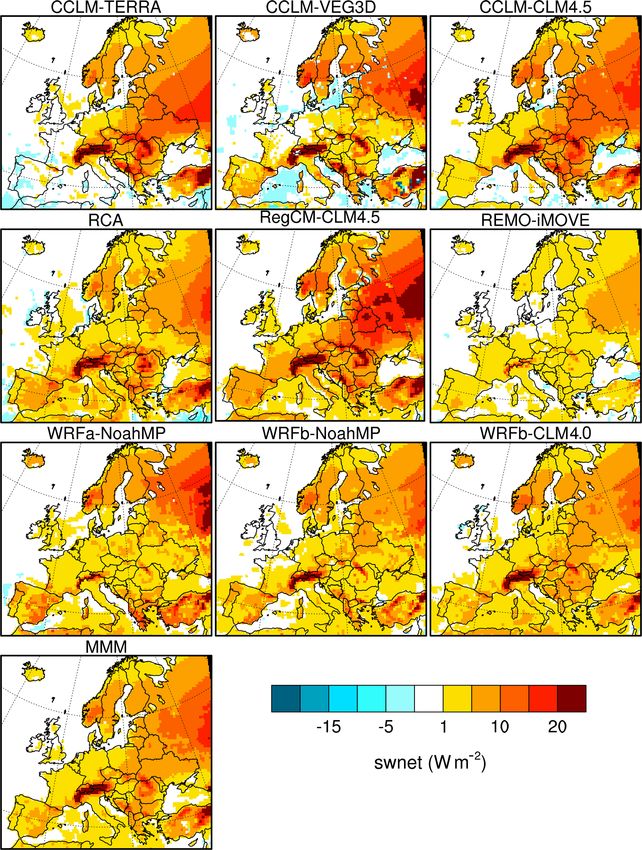
E. L. Davin et al.: Biogeophysical impacts of forestation in Europe
Figure 1. Seasonally averaged 2 m temperature (FOREST minus
models) or a mixed response (CCLM-VEG3D and CCLM-
CLM4.5). Overall this highlights the strong seasonal con-
trasts in the temperature effect of forestation and the larger
Looking separately at the response for daytime and
nighttime 2 m temperatures also indicates important diur-
nal contrasts. The winter warming effect is stronger and
more widespread for daily maximum temperature (Fig. 3),
while daily minimum temperature shows a more contrasted
cooling–warming dipole across the domain (Fig. 5). In sum-
mer, diurnal contrasts are even more pronounced with a ma-
jority of models showing an opposite sign of change for daily
maximum and minimum temperatures over most of Europe
(Figs. 4 and 6), namely a daytime warming effect and a
nighttime cooling effect. Exceptions are RCA and CCLM-
TERRA, which indicate a cooling for both daily maximum
and minimum temperatures and REMO-iMOVE exhibiting a
In terms of magnitude, the temperature signal is substan-
tial. In all RCMs, there is at least one season with abso-
lute temperature changes above 2◦ in some regions, for in-
stance in winter and spring over northern Europe (Fig. S2).
www.earth-syst-dynam.net/11/183/2020/
uncertainties associated with the summer response.
warming for both daytime and nighttime.
GRASS) for winter (DJF).
Table 1. Continued.
Model name CCLM-TERRA CCLM-VEG3D CCLM-CLM4.5 RCA RegCM-CLM4.5 REMO-iMOVE WRFa-NoahMP WRFb-NoahMP WRFb-CLM4.0
Institute ID JLU/BTU/CMCC KIT ETH SMHI ICTP GERICS IDL UHOH AUTH
RCM COSMO_5.0_clm9 COSMO_5.0_clm9 COSMO_5.0_clm9 RCA4 RegCM4.6.1 REMO2009 WRF381 WRF381 WRF381
(Giorgi et al., 2012)
Atmospheric settings
Earth Syst. Dynam., 11, 183–200, 2020
Convection scheme Tiedtke (1989) Tiedtke, (1989) Tiedtke (1989) Bechtold et al. Tiedtke (1996) for (Tiedtke, 1989) Grell and Freitas (Kain, 2004); no (Kain, 2004); no
(2001) cumulus convec- with modifications (2014) for cumulus shallow convection shallow convection
tion after Nordeng convection and
(1994) Global/Regional
Integrated Model
system (GRIMs)
Scheme (Hong
et al., 2013) for
shallow convection
Microphysics scheme one-moment cloud micro- one-moment cloud one-moment cloud values from tables Subgrid Explicit Sundqvist (1978); two-moment, six- Thompson et al. Thompson et al.
physics scheme (Seifert and microphysics microphysics Moisture scheme Roeckner et al. class scheme (Lim (2004) (2004)
Beheng, 2001) scheme (Seifert and scheme (Seifert and (SUBEX) (Pal et (1996) and Hong, 2010)
Beheng, 2001) Beheng, 2001) al., 2000)
Greenhouse gases historical (Meinshausen et al., historical (Mein- historical (Mein- historical (Mein- historical (Mein- historical (Mein- historical (Mein- constant constant
2011) shausen et al., shausen et al., shausen et al., shausen et al., shausen et al., shausen et al., (CO2 = 379 ppm) (CO2 = 379 ppm)
2011) 2011) 2011) 2011) 2011) 2011)
Aerosols constant (Tanré, 1984) Tegen et al. (1997) constant (Tanré, constant not accounted for constant (Teich- Tegen et al. (1997) Tegen et al. (1997) Tegen et al. (1997)
climatology 1984) mann et al., 2013) climatology climatology climatology
188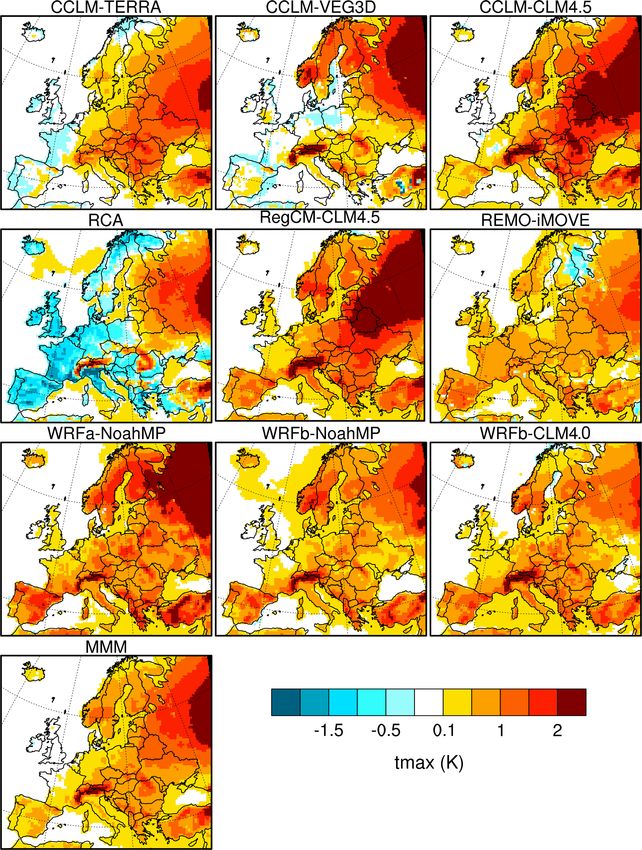
E. L. Davin et al.: Biogeophysical impacts of forestation in Europe                                                        189

Figure 2. Seasonally averaged 2 m temperature (FOREST minus       Figure 3. Seasonally averaged daily maximum 2 m temperature
GRASS) for summer (JJA).                                          (FOREST minus GRASS) for winter (DJF).

The magnitude of changes is even more pronounced for daily        incoming radiation is higher in these seasons, thus imply-
maximum temperature.                                              ing a larger surface radiation gain despite the smaller abso-
                                                                  lute change in albedo. Notable outliers are REMO-iMOVE,
3.2   Surface energy balance                                      exhibiting a smaller albedo decrease across all seasons and
                                                                  thus a less pronounced increase in net shortwave radiation,
Changes in surface energy fluxes over land are summa-             and CCLM-TERRA and RCA, which despite the albedo in-
rized for eight European regions (the Alps, the British Isles,    crease simulate a net shortwave radiation decrease in sum-
eastern Europe, France, the Iberian Peninsula, the Mediter-       mer (only over Scandinavia in the case of RCA). In the lat-
ranean, mid-Europe and Scandinavia) as defined in the PRU-        ter two models, an increase in evapotranspiration triggers an
DENCE project (Christensen et al., 2007). Here we discuss         increase in cloud cover and a subsequent decrease in incom-
results for two selected regions representative of northern Eu-   ing shortwave radiation (not shown) offsetting the change in
rope (Scandinavia; Fig. 9) and southern Europe (the Mediter-      surface albedo. The spatial pattern of surface net shortwave
ranean; Fig. 10), while results for the full set of regions are   radiation change is relatively consistent across RCMs in win-
provided in the Supplement (Figs. S11 to S18). One of the         ter with maximum net shortwave radiation increases well
most robust features across models and seasons is an increase     above 10 W m−2 in high-elevation regions and the northeast
in surface net shortwave radiation. This increase is a direct     of Europe (Fig. 7). In summer, the magnitude of net short-
consequence of the impact of forestation on surface albedo.       wave radiation changes is overall larger as is the inter-model
Indeed all RCMs consistently simulate a year-round decrease       spread (Fig. 8). CCLM-TERRA is the only RCM to simu-
in surface albedo due to the lower albedo of forest compared      late a widespread decrease in net shortwave radiation, while
to grassland (Fig. S7). This decrease is strongest in winter      RCA and CCLM-VEG3 also simulate net shortwave radia-
and at high latitudes owing to the snow-masking effect of         tion decreases in some areas in particular in northern Europe.
forest. However, the strongest increase in net shortwave ra-      All other RCMs simulate a widespread increase in net short-
diation occurs in spring and summer in both regions because       wave radiation over land, with WRFa-NoahMP and WRFb-

www.earth-syst-dynam.net/11/183/2020/                                                Earth Syst. Dynam., 11, 183–200, 2020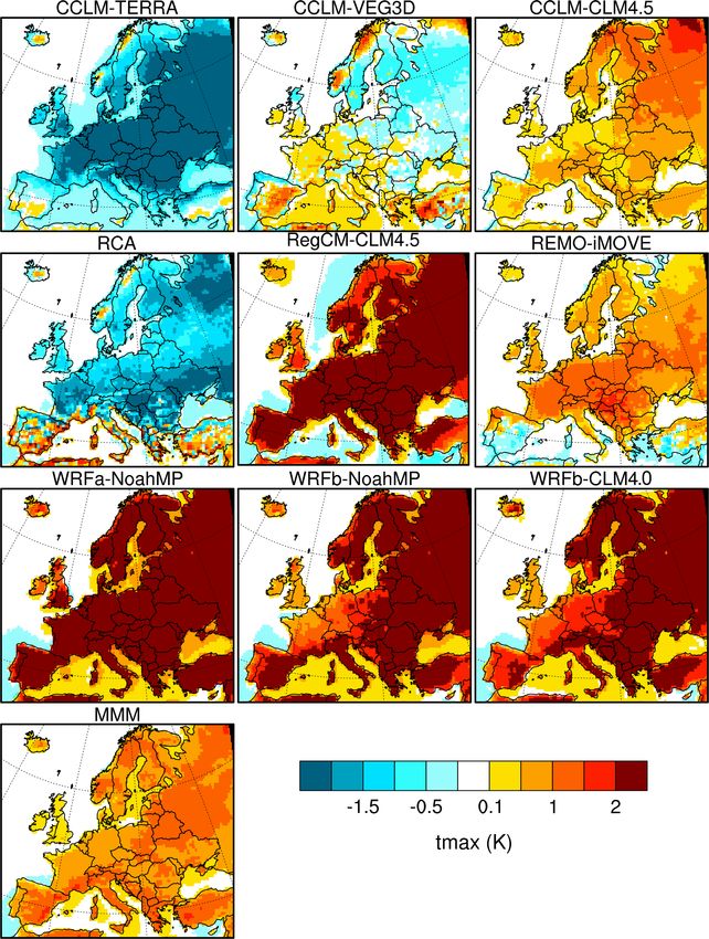
190 E. L. Davin et al.: Biogeophysical impacts of forestation in Europe
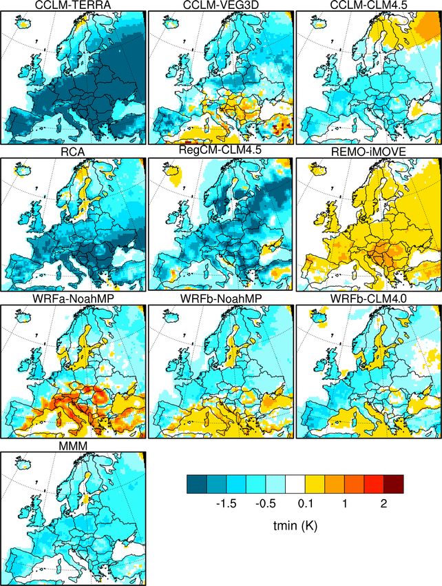
Figure 4. Seasonally averaged daily maximum 2 m temperature Figure 5. Seasonally averaged daily minimum 2 m temperature
(FOREST minus GRASS) for summer (JJA). (FOREST minus GRASS) for winter (DJF).
NoahMP exhibiting the strongest increase with values well 3.3 Origin of the inter-model spread
above 20 W m−2 in most regions.
To a large extent, sensible heat flux follows shortwave ra- Changes in albedo and in the partitioning of turbulent heat
diation changes (i.e. a majority of models suggest an increase fluxes are essential in determining the temperature effect of
in sensible heat). This is also largely the case for ground forestation. The dominant influence of albedo decrease is ev-
heat flux (calculated here indirectly as the residual of the ident in winter and spring over northern Europe as illustrated
surface energy balance), which increases in autumn, winter for instance by the quasilinear inter-model relationship be-
and spring in most models due to the overall increase in ab- tween the magnitude of changes in albedo and in 2 m temper-
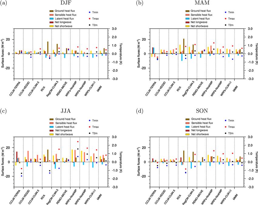
sorbed radiation. Changes in the latent heat flux exhibit a ature over Scandinavia in spring (Fig. 11a). The role of turbu-
higher degree of disagreement across models and seasons. lent heat fluxes partitioning can be illustrated by examining
For instance in spring, latent heat flux increases together with changes in evaporative fraction (EF), calculated as the ratio
sensible heat over Scandinavia (Fig. 9), while it decreases between latent heat and the sum of latent and sensible heat.
in most models over the Mediterranean (Fig. 10). In sum- The advantage of using EF instead of latent heat flux is that
mer, the agreement is low over Scandinavia, and there is the former provides a metric relatively independent of albedo
a tendency for decreasing latent heat in the Mediterranean. change (since albedo change does influence the magnitude
At the European scale, there is a clear tendency of increas- of turbulent heat fluxes through changes in available energy).
ing latent heat flux in spring particularly over northern Eu- Taking the example of Scandinavia in summer (Fig. 11b), it
rope, whereas in summer most RCMs (with the exception of appears that there is a relatively linear relationship between
CCLM-TERRA) indicate both increasing and decreasing la- changes in temperature and in EF. In other words, models
tent heat depending on regions (Fig. S10). showing a decrease in EF following forestation tend to sim-
ulate a warming and models showing an increase in EF sim-
ulate a cooling.
In order to assess more systematically the role of individ-
ual drivers across regions and seasons, we perform a regres-
Earth Syst. Dynam., 11, 183–200, 2020 www.earth-syst-dynam.net/11/183/2020/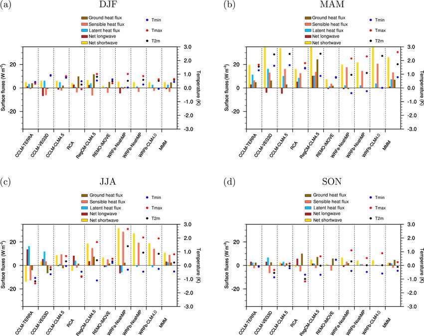
E. L. Davin et al.: Biogeophysical impacts of forestation in Europe                                                        191

Figure 6. Seasonally averaged daily minimum 2 m temperature       Figure 7. Seasonally averaged net surface shortwave radiation
(FOREST minus GRASS) for summer (JJA).                            (FOREST minus GRASS) for winter (DJF).

sion analysis using changes in albedo, EF and incoming sur-       model variance in summer over Scandinavia and in spring,
face shortwave radiation as explanatory variables and 2 m         summer and autumn over the Mediterranean. Finally, incom-
temperature as the variable to be explained. The rationale        ing surface shortwave radiation explains a substantial part
for using albedo, EF and incoming surface shortwave radi-         of the inter-model variance across most seasons although it
ation as explaining factors is that the first two capture the     is not a dominating factor. It is important to note the two
intrinsic LUC-induced changes in land surface characteris-        main caveats of this simplified approach: (1) the explanatory
tics representing respectively the radiative and non-radiative    variables are likely not fully independent due to the tightly
impacts of LUC, whereas incoming surface shortwave radi-          coupled processes in the models; (2) other factors not in-
ation captures some of the potential subsequent atmospheric       cluded as explanatory variables may contribute to the tem-
feedbacks (e.g. through cloud cover changes). Here we dis-        perature response (e.g. changes in surface roughness, other
cuss the results of the regression analysis for Scandinavia and   atmospheric feedbacks). Nevertheless, the fact that a large
the Mediterranean (Fig. 12), while results for the full set of    part of the variance can be explained by this simple linear
regions are provided in the Supplement (Figs. S19 and S20).       model is an indication of the essential role of these selected
Combining albedo, EF and incoming surface shortwave ra-           processes. An exception is the winter season during which a
diation into a multiple linear regression effectively explains    very limited part of the inter-model spread can be explained,
a large fraction of the inter-model variance of the simulated     suggesting that other processes may play a dominant role.
temperature response (around 80 % of variance explained for       One potential process that could explain differences across
both regions and all seasons except winter where the ex-          RCMs is the occurrence of precipitation feedbacks. We note
plained variance is much lower). Albedo change alone ex-          however that precipitation changes are small in all RCMs
plains the largest part of the inter-model variance in spring     with no clear consensus among models (Fig. S5). One possi-
over Scandinavia and in winter over the Mediterranean, indi-      ble exception is the summer precipitation decrease in WRFa-
cating a dominance of radiative processes during these sea-       NoahMP, which could be related to the use of the Grell–
sons. EF change alone explains the largest part of the inter-     Freitas convection scheme (Table 1), while precipitation is

www.earth-syst-dynam.net/11/183/2020/                                                Earth Syst. Dynam., 11, 183–200, 2020
192                                                         E. L. Davin et al.: Biogeophysical impacts of forestation in Europe

                                                                   tering applying the Ward’s clustering criterion (Ward, 1963).
                                                                   For the 2 m temperature response, the cluster analysis in-
                                                                   dicates a relatively high degree of similarity in winter be-
                                                                   tween RCMs sharing the same atmospheric scheme, as il-
                                                                   lustrated in particular by the clustering of CCLM-TERRA
                                                                   and CCLM-CLM4.5 and of WRFb-NoahMP and WRFb-
                                                                   CLM4.0 (Fig. 13). In contrast, CCLM-TERRA and CCLM-
                                                                   CLM4.5 are relatively far apart in summer suggesting a
                                                                   stronger influence of land processes during this season. This
                                                                   tendency, however, does not arise in the WRF-based RCMs,
                                                                   with WRFb-NoahMP and WRFb-CLM4.0 showing a high
                                                                   degree of similarity even in summer. A possible explanation
                                                                   could be that NoahMP and CLM4.0 are structurally less dif-
                                                                   ferent than TERRA and CLM4.5.

                                                                   4   Discussion and conclusions

                                                                   Results from nine RCMs show that, compared to grassland,
                                                                   forests imply warmer temperatures in winter and spring over
                                                                   northern Europe. This result is robust across RCMs and is
                                                                   a direct consequence of the lower albedo of forests, which
                                                                   is the dominating factor during these seasons. In summer
                                                                   and autumn, however, the RCMs disagree on the direction
                                                                   of changes, with responses ranging from a widespread cool-
                                                                   ing to a widespread warming above 2◦ in both cases. Al-
                                                                   though albedo change plays an important role in all seasons
                                                                   by increasing absorbed surface radiation, in summer inter-
Figure 8. Seasonally averaged net surface shortwave radiation      model differences in the temperature response are to a large
(FOREST minus GRASS) for summer (JJA).
                                                                   extent induced by differences in EF. These conclusions are
                                                                   overall consistent with previous studies based on global cli-
                                                                   mate models. Results from the LUCID and the CMIP5 model
less affected in WRFb-NoahMP and WRFb-CLM4.0, which                intercomparisons have indeed highlighted a robust, albedo-
use the Kain–Fritsch scheme. The stronger summer tem-              induced, winter cooling effect due to past deforestation at
perature increase in WRFa-NoahMP compared to WRFb-                 mid-latitudes (Lejeune et al., 2017), in other words implying
NoahMP and WRFb-CLM4.0 may therefore be linked to this             a winter warming effect of forestation. On the other hand,
precipitation feedback.                                            no robust summer response has been identified in these inter-
   Comparing results from different RCMs sharing either the        comparisons, mainly attributed to a lack of agreement across
same LSM or the same atmospheric model can help pro-               models concerning evapotranspiration changes (Lejeune et
vide additional insights into the respective role of land versus   al., 2017, 2018; de Noblet-Ducoudré et al., 2012).
atmospheric processes. By comparing for instance the tem-             Resolving this lack of consensus will require intensified
perature response across RCMs (Figs. 1 to 6), it appears, in       efforts to confront models and observations and identify pos-
summer particularly, that the three RCMs based on CCLM             sible model deficiencies (Boisier et al., 2013, 2014; Duveiller
(i.e. same atmospheric model with three different LSMs)            et al., 2018a; Meier et al., 2018). For instance, a key feature
span almost the full range of RCM responses while CCLM-            emerging from observation-based studies is the fact that mid-
CLM4.5 and RegCM-CLM4.5 (i.e. same LSM and differ-                 latitude forests are colder during the day and warmer dur-
ent atmospheric models) have generally similar patterns of         ing the night compared to grassland (Duveiller et al., 2018b;
change. This suggests that the summer temperature response         Lee et al., 2011; Li et al., 2015). It is striking that none of
to forestation is conditioned primarily by land process repre-     the LUCID and CMIP5 models reflect this diurnal behaviour
sentation more than by atmospheric processes. To quantify          (Lejeune et al., 2017), nor do the RCMs analysed in this
objectively the level of similarity or dissimilarity between       study (i.e. a majority of RCMs have a diurnal signal op-
different RCMs, we compute the Euclidean distance across           posite to observations, two other RCMs indicate a cooling
latitude and longitude between each RCM pairs for each sea-        effect of forests for both day and night, and one exhibits a
son for differences in 2 m temperature and precipitation. This     warming effect for both day and night). It is however im-
distance matrix is then used as a basis for a hierarchical clus-   portant to note that this apparent contradiction may not be

Earth Syst. Dynam., 11, 183–200, 2020                                                www.earth-syst-dynam.net/11/183/2020/
E. L. Davin et al.: Biogeophysical impacts of forestation in Europe 193 Figure 9. Changes in temperature and in surface energy balance components (FOREST minus GRASS) averaged over Scandinavia for DJF, MAM, JJA and SON. Results for other regions are shown in the Supplement. only attributable to model deficiencies and could be in part under equivalent soil moisture conditions) in particular due related to discrepancies on the scale of processes considered to unrealistic choices of root distribution, photosynthetic pa- in models and observations. Indeed, observation-based esti- rameters and water uptake formulation. After improvement mates capture mainly local changes in surface energy balance of these aspects in CLM4.5, evapotranspiration was found to and temperature due to land cover and are unlikely to reflect be more realistically simulated, also resulting in an improved the type of large-scale atmospheric feedbacks triggered in daytime temperature difference between grassland and for- coupled climate models (especially given the large-scale na- est (Meier et al., 2018). An important insight from this first ture of the forest expansion considered in our experiments). phase of RCM experiments is therefore that particular atten- Similarly, the fact that a majority of RCMs simulate a sum- tion should be given to model evaluation and benchmarking mer decrease in evapotranspiration over many regions fol- in future phases of the LUCAS initiative. lowing forestation is at odds with current observational evi- An additional insight from this study concerns the role dence (Chen et al., 2018; Duveiller et al., 2018b; Meier et al., of land versus atmospheric processes. Some of the partici- 2018) and might play a role in the simulated summer daytime pating RCMs share the same atmospheric scheme (i.e. the warming in most RCMs. Although the reasons behind this same version and configuration) but are coupled to different behaviour may be model-specific, some recent work based on land surface models or share the same land surface model in the CLM4.5 model, which is used in two of the RCMs here, combination with different atmospheric schemes. This repre- sheds some light on the possible processes involved (Meier sents a unique opportunity to objectively determine the origin et al., 2018). It was found that while evapotranspiration is of uncertainties in the simulated response. For instance, we higher in spring under forested conditions in CLM4.5, trees find that land process representation is heavily involved in become more water stressed than grassland in summer (even the large model spread in summer temperature response. The www.earth-syst-dynam.net/11/183/2020/ Earth Syst. Dynam., 11, 183–200, 2020
194                                                         E. L. Davin et al.: Biogeophysical impacts of forestation in Europe

Figure 10. Changes in temperature and in surface energy balance components (FOREST minus GRASS) averaged over the Mediterranean
for DJF, MAM, JJA and SON. Results for other regions are shown in the Supplement.

Figure 11. Illustrative relationships between changes (FOREST minus GRASS) in 2 m temperature and albedo in spring (a) and between
changes in 2 m temperature and EF (evaporative fraction) in summer (b) for Scandinavia.

Earth Syst. Dynam., 11, 183–200, 2020                                                 www.earth-syst-dynam.net/11/183/2020/
E. L. Davin et al.: Biogeophysical impacts of forestation in Europe                                                                    195

Figure 12. Fraction of inter-model variance in 2 m temperature change (FOREST minus GRASS) explained by changes in albedo, evapora-
tive fraction, incoming surface shortwave radiation or the three combined. Alb: inter-model correlation (Rsquared) between changes in albedo
and 2 m temperature. EF: inter-model correlation (Rsquared) between changes in evaporative fraction and 2 m temperature. SWin: inter-
model correlation (Rsquared) between changes in incoming surface shortwave radiation and 2 m temperature. Alb + EF + SWin: Rsquared
of a multi-linear regression combining the three predictors. Results for other regions are shown in the Supplement.

Figure 13. Dendrogram of the clustering analysis based on the 2 m temperature response (FOREST minus GRASS) for DJF and JJA. The
underlying distance matrix between RCM pairs is based on the Euclidean distance across latitude and longitude for the given season.

range of responses generated by using three different LSMs              nevertheless also play a substantial or even dominant role for
within the same atmospheric scheme (CCLM) is almost as                  example in winter or for other variables such as precipitation.
large as the full model range in summer. Supporting this con-              In this first phase of LUCAS, we relied on idealized exper-
clusion, a simple regression-based analysis shows that, ex-             iments at relatively low resolution (50 km) to gain insights
cept in winter, changes in albedo and EF can explain most               into the biogeophysical role of forests across a range of Eu-
of the inter-model spread in temperature sensitivity, in other          ropean climates. Future phases of LUCAS will evolve to-
words indicating that land processes primarily determine the            ward increasing realism for instance by (1) investigating tran-
simulated temperature response. Atmospheric processes can               sient historical LUC forcing as well as RCP (representative
                                                                        concentration pathways)-based LUC scenarios, (2) consider-

www.earth-syst-dynam.net/11/183/2020/                                                        Earth Syst. Dynam., 11, 183–200, 2020
196 E. L. Davin et al.: Biogeophysical impacts of forestation in Europe
ing a range of land use transitions beyond grassland to for- Susanna Strada has been supported by the TALENTS3 Fellowship
est conversion and (3) assessing the added-value of higher Programme (FP code 1718349004) funded by the autonomous re-
(kilometre-scale) resolution when assessing local LUC im- gion Friuli Venezia Giulia via the European Social Fund (Oper-
pacts. Finally, the most societally relevant adverse effects or ative Regional Programme 2014–2020) and administered by the
benefits from land management strategies may become ap- AREA Science Park (Padriciano, Italy). CCLM-TERRA simula-
tions were performed at the German Climate Computing Center
parent only when addressing changes in extreme events such
(DKRZ) through support from the Federal Ministry of Education
as heatwaves or droughts (Davin et al., 2014; Lejeune et al., and Research in Germany (BMBF). Merja H. Tölle acknowledges
2018), an aspect which will receive more attention in future the funding of the German Research Foundation (DFG) through
analyses based on LUCAS simulations. grant 401857120. We thank Richard Wartenburger for providing
the R scripts that have been used to perform the cluster analysis.
We acknowledge the support of LUCAS by WCRP-CORDEX as a
Data availability. The data and scripts used are available upon re- Flagship Pilot Study.
quest from the corresponding author.
Financial support. This research has been supported by the
Supplement. The supplement related to this article is available Swiss National Science Foundation (grant no. 200021_172715).
online at: https://doi.org/10.5194/esd-11-183-2020-supplement.
Review statement. This paper was edited by Somnath Baidya
Author contributions. ELD, DR, MB, RMC, EC, PH, LLJ, EK, Roy and reviewed by two anonymous referees.
KR, MR, PMMS, GS, SS, GS, MHT and KWS performed the RCM
simulations, using vegetation maps produced by ELD. ELD de-
signed the research, analysed the data and wrote the paper. All au-
thors contributed to interpreting the results and revising the text. References
Bechtold, P., Bazile, E., Guichard, F., Mascart, P., and
Richard, E.: A mass-flux convection scheme for regional
Competing interests. The authors declare that they have no con-
and global models, Q. J. Roy. Meteor. Soc., 127, 869–886,
flict of interest.
https://doi.org/10.1002/qj.49712757309, 2001.
Boisier, J. P., de Noblet-Ducoudré, N., and Ciais, P.: Inferring
past land use-induced changes in surface albedo from satel-
Acknowledgements. Edouard L. Davin acknowledges support lite observations: a useful tool to evaluate model simulations,
from the Swiss National Science Foundation (SNSF) through the Biogeosciences, 10, 1501–1516, https://doi.org/10.5194/bg-10-
CLIMPULSE project and thanks the Swiss National Supercomput- 1501-2013, 2013.
ing Centre (CSCS) for providing computing resources. Rita M. Car- Boisier, J. P., de Noblet-Ducoudré, N., and Ciais, P.: Historical land-
doso and Pedro M. M. Soares acknowledge the projects LEADING use-induced evapotranspiration changes estimated from present-
(PTDC/CTA-MET/28914/2017) and FCT- UID/GEO/50019/2019 day observations and reconstructed land-cover maps, Hydrol.
– Instituto Dom Luiz. Peter Hoffmann is funded by the Cli- Earth Syst. Sci., 18, 3571–3590, https://doi.org/10.5194/hess-18-
mate Service Center Germany (GERICS) of the Helmholtz- 3571-2014, 2014.
Zentrum Geesthacht in the frame of the HICSS (Helmholtz-Institut Bonan, G. B.: Forests and climate change: Forcings, feedbacks,
Climate Service Science) project LANDMATE. Lisa L. Jach, and the climate benefits of forests, Science, 320, 1444–1449,
Kirsten Warrach-Sagi and Volker Wulfmeyer acknowledge sup- https://doi.org/10.1126/science.1155121, 2008.
port by the state of Baden-Württemberg through bwHPC and Breil, M., Schädler, G. and Laube, N.: An Improved Soil
thank the Anton and Petra Ehrmann-Stiftung Research Training Moisture Parametrization for Regional Climate Simula-
Group “Water-People-Agriculture” for financial support. The work tions in Europe, J. Geophys. Res.-Atmos., 123, 7331–7339,
of Eleni Katragkou and Giannis Sofiadis was supported by com- https://doi.org/10.1029/2018JD028704, 2018.
putational time granted from the Greek Research & Technology Bretherton, C. S., McCaa, J. R., Grenier, H., Bretherton,
Network (GRNET) in the National HPC facility – ARIS – under C. S., McCaa, J. R. and Grenier, H.: A New Parame-
project ID pr005025_thin. Nathalie de Noblet-Ducoudré thanks the terization for Shallow Cumulus Convection and Its Ap-
“Investments d’Avenir” Programme overseen by the French Na- plication to Marine Subtropical Cloud-Topped Bound-
tional Research Agency (ANR) (LabEx BASC; ANR-11-LABX- ary Layers. Part I: Description and 1D Results, Mon.
0034). RCA simulations were performed on the Swedish climate Weather Rev., 132, 864–882, https://doi.org/10.1175/1520-
computing resource Bi provided by the Swedish National Infras- 0493(2004)1322.0.CO;2, 2004.
tructure for Computing (SNIC) at the Swedish National Supercom- Chen, L., Dirmeyer, P. A., Guo, Z., and Schultz, N. M.: Pair-
puting Centre (NSC) at Linköping University. G. Strandberg was ing FLUXNET sites to validate model representations of land-
partly funded by a research project financed by the Swedish Re- use/land-cover change, Hydrol. Earth Syst. Sci., 22, 111–125,
search Council VR (Vetenskapsrådet) on “Quantification of the bio- https://doi.org/10.5194/hess-22-111-2018, 2018.
geophysical and biogeochemical forcings from anthropogenic de- Cherubini, F., Huang, B., Hu, X., Tölle, M. H., and Strømman,
forestation on regional Holocene climate in Europe, LandClim II”. A. H.: Quantifying the climate response to extreme land cover
Earth Syst. Dynam., 11, 183–200, 2020 www.earth-syst-dynam.net/11/183/2020/E. L. Davin et al.: Biogeophysical impacts of forestation in Europe 197 changes in Europe with a regional model, Environ. Res. Lett., for the assessment of the biogeophysical effects of a poten- 13, 074002, https://doi.org/10.1088/1748-9326/aac794, 2018. tial afforestation in Europe, Carbon Balance Manag., 8, 3, Christensen, J. H. and Christensen, O. B.: A summary of the https://doi.org/10.1186/1750-0680-8-3, 2013. PRUDENCE model projections of changes in European cli- Giorgi, F., Bates, G. T., Giorgi, F., and Bates, G. T.: The Climato- mate by the end of this century, Climatic Change, 81, 7–30, logical Skill of a Regional Model over Complex Terrain, Mon. https://doi.org/10.1007/s10584-006-9210-7, 2007. Weather Rev., 117, 2325–2347, https://doi.org/10.1175/1520- Christensen, J. H., Carter, T. R., Rummukainen, M., and Amana- 0493(1989)1172.0.CO;2, 1989. tidis, G.: Evaluating the performance and utility of regional cli- Giorgi, F., Marinucci, M. R., Bates, G. T., De Canio, G., mate models: the PRUDENCE project, Climatic Change, 81, 1– Giorgi, F., Marinucci, M. R., Bates, G. T., and Canio, 6, https://doi.org/10.1007/s10584-006-9211-6, 2007. G. De: Development of a Second-Generation Regional Claussen, M., Brovkin, V., and Ganopolski, A.: Biogeophysical ver- Climate Model (RegCM2). Part II: Convective Processes sus biogeochemical feedbacks of large-scale land cover change, and Assimilation of Lateral Boundary Conditions, Mon. Geophys. Res. Lett., 28, 1011–1014, 2001. Weather Rev., 121, 2814–2832, https://doi.org/10.1175/1520- Davies, H. C.: A lateral boundary formulation for multi-level 0493(1993)1212.0.CO;2, 1993. prediction models, Q. J. Roy. Meteor. Soc., 102, 405–418, Giorgi, F., Coppola, E., Solmon, F., Mariotti, L., Sylla, M., Bi, https://doi.org/10.1002/qj.49710243210, 1976. X., Elguindi, N., Diro, G., Nair, V., Giuliani, G., Turuncoglu, Davin, E. L. and de Noblet-Ducoudré, N.: Climatic U., Cozzini, S., Güttler, I., O’Brien, T., Tawfik, A., Shal- impact of global-scale Deforestation: Radiative ver- aby, A., Zakey, A., Steiner, A., Stordal, F., Sloan, L., and sus nonradiative processes, J. Climate, 23, 97–112, Brankovic, C.: RegCM4: model description and preliminary https://doi.org/10.1175/2009JCLI3102.1, 2010. tests over multiple CORDEX domains, Clim. Res., 52, 7–29, Davin, E. L., Seneviratne, S. I., Ciais, P., Olioso, A., and https://doi.org/10.3354/cr01018, 2012. Wang, T.: Preferential cooling of hot extremes from cropland Grassi, G., House, J., Dentener, F., Federici, S., Den Elzen, M., and albedo management, P. Natl. Acad. Sci. USA, 111, 9757–9761, Penman, J.: The key role of forests in meeting climate targets https://doi.org/10.1073/pnas.1317323111, 2014. requires science for credible mitigation, Nat. Clim. Change, 7, Davin, E. L., Maisonnave, E., and Seneviratne, S. I.: Is land sur- 220–228, https://doi.org/10.1038/nclimate3227, 2017. face processes representation a possible weak link in current Grell, G. A. and Freitas, S. R.: A scale and aerosol aware Regional Climate Models?, Environ. Res. Lett., 11, 074027, stochastic convective parameterization for weather and air https://doi.org/10.1088/1748-9326/11/7/074027, 2016. quality modeling, Atmos. Chem. Phys., 14, 5233–5250, Dee, D. P., Uppala, S. M., Simmons, A. J., Berrisford, P., Poli, https://doi.org/10.5194/acp-14-5233-2014, 2014. P., Kobayashi, S., Andrae, U., Balmaseda, M. A., Balsamo, G., Grenier, H., Bretherton, C. S., Grenier, H., and Bretherton, C. S.: A Bauer, P., Bechtold, P., Beljaars, A. C. M., van de Berg, L., Bid- Moist PBL Parameterization for Large-Scale Models and Its Ap- lot, J., Bormann, N., Delsol, C., Dragani, R., Fuentes, M., Geer, plication to Subtropical Cloud-Topped Marine Boundary Layers, A. J., Haimberger, L., Healy, S. B., Hersbach, H., Holm, E. V, Mon. Weather Rev., 129, 357–377, https://doi.org/10.1175/1520- Isaksen, L., Kallberg, P., Koehler, M., Matricardi, M., McNally, 0493(2001)1292.0.CO;2, 2001. A. P., Monge-Sanz, B. M., Morcrette, J.-J., Park, B.-K., Peubey, Griscom, B. W., Adams, J., Ellis, P. W., Houghton, R. A., Lomax, C., de Rosnay, P., Tavolato, C., Thepaut, J.-N., and Vitart, F.: The G., Miteva, D. A., Schlesinger, W. H., Shoch, D., Siikamaki, J. ERA-Interim reanalysis: configuration and performance of the V, Smith, P., Woodbury, P., Zganjar, C., Blackman, A., Campari, data assimilation system, Q. J. Roy. Meteor. Soc., 137, 553–597, J., Conant, R. T., Delgado, C., Elias, P., Gopalakrishna, T., Ham- https://doi.org/10.1002/qj.828, 2011. sik, M. R., Herrero, M., Kiesecker, J., Landis, E., Laestadius, L., de Noblet-Ducoudré, N., Boisier, J.-P., Pitman, A., Bonan, G. B., Leavitt, S. M., Minnemeyer, S., Polasky, S., Potapov, P., Putz, F. Brovkin, V., Cruz, F., Delire, C., Gayler, V., van den Hurk, B. E., Sanderman, J., Silvius, M., Wollenberg, E., and Fargione, J.: J. J. M., Lawrence, P. J., van der Molen, M. K., Mueller, C., Natural climate solutions, P. Natl. Acad. Sci. USA, 114, 11645– Reick, C. H., Strengers, B. J., and Voldoire, A.: Determining 11650, https://doi.org/10.1073/pnas.1710465114, 2017. Robust Impacts of Land-Use-Induced Land Cover Changes on Gutowski Jr., W. J., Giorgi, F., Timbal, B., Frigon, A., Jacob, D., Surface Climate over North America and Eurasia: Results from Kang, H.-S., Raghavan, K., Lee, B., Lennard, C., Nikulin, G., the First Set of LUCID Experiments, J. Climate, 25, 3261–3281, O’Rourke, E., Rixen, M., Solman, S., Stephenson, T., and Tan- https://doi.org/10.1175/JCLI-D-11-00338.1, 2012. gang, F.: WCRP COordinated Regional Downscaling EXperi- Duveiller, G., Forzieri, G., Robertson, E., Li, W., Georgievski, ment (CORDEX): a diagnostic MIP for CMIP6, Geosci. Model G., Lawrence, P., Wiltshire, A., Ciais, P., Pongratz, J., Sitch, Dev., 9, 4087–4095, https://doi.org/10.5194/gmd-9-4087-2016, S., Arneth, A., and Cescatti, A.: Biophysics and vegetation 2016. cover change: a process-based evaluation framework for con- Harper, A. B., Powell, T., Cox, P. M., House, J., Huntingford, C., fronting land surface models with satellite observations, Earth Lenton, T. M., Sitch, S., Burke, E., Chadburn, S. E., Collins, W. Syst. Sci. Data, 10, 1265–1279, https://doi.org/10.5194/essd-10- J., Comyn-Platt, E., Daioglou, V., Doelman, J. C., Hayman, G., 1265-2018, 2018a. Robertson, E., van Vuuren, D., Wiltshire, A., Webber, C. P., Bas- Duveiller, G., Hooker, J., and Cescatti, A.: The mark of vegetation tos, A., Boysen, L., Ciais, P., Devaraju, N., Jain, A. K., Krause, change on Earth’s surface energy balance, Nat. Commun., 9, 679, A., Poulter, B., and Shu, S.: Land-use emissions play a criti- 3261–3281, https://doi.org/10.1038/s41467-017-02810-8, 2018. cal role in land-based mitigation for Paris climate targets, Nat. Gálos, B., Hagemann, S., Hänsler, A., Kindermann, G., Rechid, Commun., 9, 2938, https://doi.org/10.1038/s41467-018-05340- D., Sieck, K., Teichmann, C., and Jacob, D.: Case study z, 2018. www.earth-syst-dynam.net/11/183/2020/ Earth Syst. Dynam., 11, 183–200, 2020
You can also read