Retrieval of process rate parameters in the general dynamic equation for aerosols using Bayesian state estimation: BAYROSOL1.0 - GMD
←
→
Page content transcription
If your browser does not render page correctly, please read the page content below
Geosci. Model Dev., 14, 3715–3739, 2021
https://doi.org/10.5194/gmd-14-3715-2021
© Author(s) 2021. This work is distributed under
the Creative Commons Attribution 4.0 License.

Retrieval of process rate parameters in the general dynamic
equation for aerosols using Bayesian state estimation:
BAYROSOL1.0
Matthew Ozon1 , Aku Seppänen1 , Jari P. Kaipio1,3 , and Kari E. J. Lehtinen1,2
1 Department of Applied Physics, University of Eastern Finland, Kuopio, Finland
2 FinnishMeteorological Institute, Kuopio, Finland
3 Department of Mathematics, Faculty of Science, University of Auckland, Auckland, New Zealand

Correspondence: Matthew Ozon (matthew.ozon@uef.fi)

Received: 16 July 2020 – Discussion started: 16 October 2020
Revised: 24 March 2021 – Accepted: 5 May 2021 – Published: 22 June 2021

Abstract. The uncertainty in the radiative forcing caused by      manathan et al., 2001). Worldwide, particulate air pollutants
aerosols and its effect on climate change calls for research      are also responsible for up to 7 million premature deaths
to improve knowledge of the aerosol particle formation and        per year (WHO 2014). The Intergovernmental Panel on Cli-
growth processes. While experimental research has provided        mate Change (IPCC Assessment Report 2013 by Stocker et
a large amount of high-quality data on aerosols over the last     al., 2014, and IPCC Assessment Report 2014 by Pachauri
2 decades, the inference of the process rates is still inade-     et al., 2014) recognized the uncertainty in the radiative forc-
quate, mainly due to limitations in the analysis of data. This    ing caused by aerosols as the main individual factor limit-
paper focuses on developing computational methods to infer        ing the scientific understanding of future and past climate
aerosol process rates from size distribution measurements. In     changes.
the proposed approach, the temporal evolution of aerosol size        Some of the uncertainty is caused by the fact that the ini-
distributions is modeled with the general dynamic equation        tial stages of the new particle formation (NPF) processes
(GDE) equipped with stochastic terms that account for the         in the atmosphere are still not completely known. It has
uncertainties of the process rates. The time-dependent parti-     been known for close to 100 years that photochemically
cle size distribution and the rates of the underlying formation   driven NPF may occur in the atmosphere (Aitken, 1889).
and growth processes are reconstructed based on time series       The fact that it occurs regularly throughout the troposphere
of particle analyzer data using Bayesian state estimation –       has, however, only become clear during the last 15 years or
which not only provides (point) estimates for the process         so (Kulmala et al., 2004). Partly because of this, the sys-
rates but also enables quantification of their uncertainties.     tematic development of parameterizations describing tropo-
The feasibility of the proposed computational framework is        spheric NPF as an active research topic has only just begun.
demonstrated by a set of numerical simulation studies.            Studies with these models suggest that tropospheric NPF
                                                                  may have significant effects on CCN and, in turn, on the
                                                                  general global cloud albedo effects of atmospheric aerosols
                                                                  (Merikanto et al., 2010). One challenge in estimating the an-
1   Introduction                                                  thropogenic aerosol effect on climate is the need to know the
                                                                  preindustrial conditions and dynamics, which is the baseline
Aerosols scatter and absorb solar radiation and affect the        of forcing estimations (Hansen et al., 1981). Very recently,
permeability of the atmosphere to solar energy (the direct        Gordon et al. (2016) made new estimations of anthropogenic
effect). In addition, aerosol particles act as seeds for cloud    aerosol radiative forcing by assuming pure biogenic particle
droplets (cloud condensation nuclei, CCN) and, thus, influ-       formation, as suggested by Kirkby et al. (2016) based on the
ence the properties of clouds (the indirect effect; e.g., Ra-     Cosmics Leaving Outdoor Droplets (CLOUD) experiment at

Published by Copernicus Publications on behalf of the European Geosciences Union.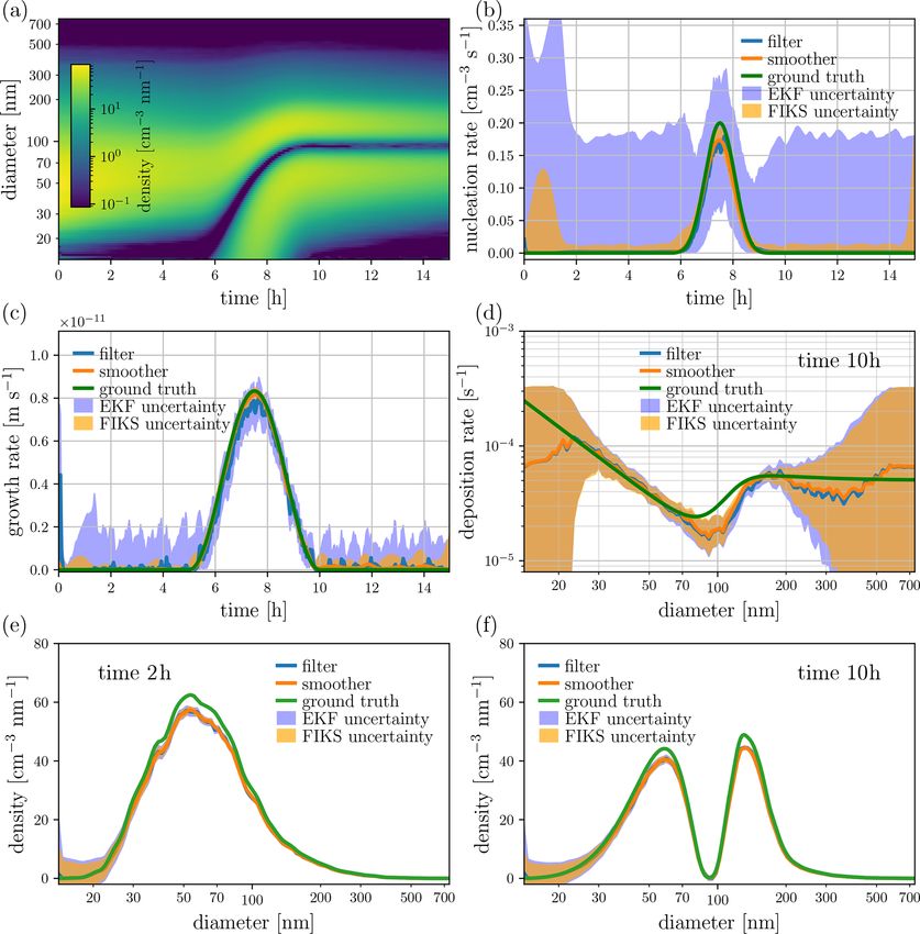
3716                                          M. Ozon et al.: Retrieval of process rate parameters in the GDE for aerosols

CERN. The increased particle formation rates under prein-         2012), suffering from potentially crude approximations and
dustrial conditions increased the CCN conditions as well as       permitting no proper estimation of the uncertainties. It is
the cloud albedo – resulting in a 0.22 W m−2 decrease in an-      likely that there are significant inaccuracies in quantities such
thropogenic aerosol forcing. As the NPF treatment in global       as particle formation and growth rates estimated previously,
climate models is typically based on parameterizing particle      and at least their uncertainties have typically not been quanti-
formation and growth rates (GRs) from chamber experiments         fied. Very recent studies by Kürten et al. (2018) have already
such as CLOUD or from field measurements, it is of great          shown that the difference between nucleation rates estimated
importance to analyze the data with care and pay attention to     by fitting a sophisticated aerosol model to data and a “tradi-
uncertainties.                                                    tional” simple method can be as large as a factor of 10.
   Most of the research dealing with NPF event analysis has          Studies on applying computational inversion methods to
used similar methodology as outlined in the “protocol” de-        estimating the most important quantities of interest with re-
scribed by Kulmala et al. (2012) and Dada et al. (2020).          spect to particle fate and effects in the atmosphere, the for-
Particle formation rates, at the detection limit of the instru-   mation and growth rates, are rare. Lehtinen et al. (2004)
ment (typically in the range from 2 to 3 nm), are usually         applied simple least-squares-based optimization of aerosol
estimated from the time evolution of either the total num-        microphysics to measured data. This method was later im-
ber concentration or the number concentration below a cer-        proved (more processes, less assumptions) by Verheggen and
tain size (e.g., 20 nm), correcting for coagulation loss and      Mozurkewich (2006) and Kuang et al. (2012). These studies,
condensation growth with very simple and approximate bal-         however, did not address the uncertainties in the estimated
ance equations. For condensational growth rate, there have        parameters. Henze et al. (2004) used the method of adjoint
been three main approaches: (1) fitting the growing nucle-        equations to estimate condensation rates based on measured
ation mode with a lognormal function, and the growth of the       evolution of the aerosol size distribution. Sandu et al. (2005)
mode GR is defined as the growth of the geometric mean            presented adjoint equations of the complete aerosol general
size of the mode (Leppä et al., 2011); (2) the so-called “max-    dynamic equation (GDE) which could be a basis for data-
imum concentration method” in which GR is estimated from          assimilation of aerosol dynamics. We are, however, not aware
the times when each measurement channel of the instrument         of the methodology being used later.
reaches its maximum concentration (Lehtinen and Kulmala,             In the statistical (Bayesian) framework of inverse prob-
2003); and (3) the so-called “appearance time method” in          lems (Kaipio and Somersalo, 2006), the uncertainties of the
which GR is estimated from concentration rise times of each       model quantities are modeled statistically, and it offers an
channel (Lehtipalo et al., 2014). Methods 1 and 2 are applica-    approach to uncertainty quantification, in addition to param-
ble to cases in which there is a clear nucleation mode grow-      eter estimation. In a time-invariant case, the Bayesian ap-
ing, as is the case, for example, for the multitude of events     proach was adopted to estimate aerosol size distributions by
analyzed from the Hyytiälä forest station in Finland (Maso        Voutilainen et al. (2001). Thus far, the only works where the
et al., 2005). For chamber experiments, where the aerosol         statistical approach has been taken to inverse problems in
size distribution approaches steady state (Dada et al., 2020),    aerosol size distribution dynamics are those on parameter es-
these two approaches cannot be used. Method 3 can then be         timation in aggregation–fragmentation models (Ramachan-
applied to the transition stage of the dynamics, before steady-   dran and Barton, 2010; Bortz et al., 2015; Shcherbacheva
state is reached. All of these methods suffer from distur-        et al., 2020), estimating the size distribution evolution us-
bances by other aerosol microphysical processes (e.g., coag-      ing Kalman filtering (Voutilainen and Kaipio, 2002; Viskari
ulation and deposition) and, in addition, cannot be used to es-   et al., 2012) and estimating evaporation rates using a Markov
timate uncertainties related to GR. Deposition rates are typ-     chain Monte Carlo method (Kupiainen-Määttä, 2016). How-
ically estimated by targeted experiments with either several      ever, the statistical inversion framework (and Bayesian state
different experiments with different monodisperse aerosol or      estimation in particular) has been applied to several other
in the absence of vapors and with low enough concentrations       problems which are mathematically similar to parameter esti-
that other microphysical processes do not affect the estima-      mation in aerosol dynamics. Unknown coefficients have been
tion.                                                             estimated in, for example, Fokker–Planck equations (Banks
   The last decade has been a huge leap forward in atmo-          et al., 1993; Dimitriu, 2002), age-structured population dy-
spheric NPF research. Instrument development, especially          namics models (Rundell, 1993; Cho and Kwon, 1997) as
advances in particle detection efficiency and mass spectrom-      well as algal and phytoplankton aggregation models (Ack-
etry, have allowed us to measure details of the dynamics          leh, 1997; Ackleh and Miller, 2018).
of the smallest clusters (e.g., Almeida et al., 2013). At the        In this paper, we approach the problem of estimating un-
same time, however, potentially superior advanced data anal-      known rate parameters in the aerosol general dynamic equa-
ysis methods have not been used. Instead, NPF and particle        tion in the framework of Bayesian state estimation. We model
growth rates have been analyzed with the abovementioned           the discretized particle size distribution as well as the un-
very simple regression or balance equation approaches (an         known nucleation, growth and deposition rates in GDE as
overview of the typical methods is given in Kulmala et al.,       multivariate random processes, and estimate them from se-

Geosci. Model Dev., 14, 3715–3739, 2021                                            https://doi.org/10.5194/gmd-14-3715-2021
M. Ozon et al.: Retrieval of process rate parameters in the GDE for aerosols                                                            3717

quential particle counter measurements using the extended                   flux, in particle-size space (cm−3 s−1 ), as a boundary con-
Kalman filter (EKF) and fixed interval Kalman smoother                      dition for the GDE. Hence, the nucleation J = J (t) is iden-
(FIKS). The feasibility of these estimators to quantify the                 tified with the flux of particles to the smallest size class by
process rate parameters and their uncertainties is tested with              condensation – that is,
series of numerical simulation studies.
                                                                            g dpmin , t n dpmin , t = J (t).                            (2)

2   Estimation of parameters in GDE                                         Similarly, for the outward flux of particles at the largest size
                                                                            class, we write
The temporal evolution of the aerosol size distribution n =
n(dp , t) can be described by a population balance equation                 g dp∞ , t n dp∞ , t = 0,                                     (3)
referred to as the GDE (Zhang et al., 1999; Prakash et al.,
2003; Lehtinen and Zachariah, 2001; Smoluchowski, 1916;                     which states that the growth of particles to a size exceeding
Friedlander and Wang, 1966). We write the continuous form                   dp∞ , the upper limit of the size range, is negligible.
of the GDE as                                                                  The time- and/or size-dependent parameters g, β, λ and J
                                                                            characterize the microphysical properties of aerosols: these
∂n              ∂g(dp , t)n(dp , t)                                         parameters, along with boundary conditions of the GDE,
   (dp , t) = −
∂t                     ∂dp                                                  completely determine the evolution of the aerosol size distri-
                                                                            bution. However, the process rate parameters are usually not
                |       {z        }
                      growth by condensation
                                                                            known. In this paper, we aim at estimating the growth, depo-
                    Z∞
                                                                            sition and nucleation rates (g, λ and J , respectively) based
    − n(dp , t)           β(dp , s)n(s, t)ds
                                                                            on particle size distribution measurements. For the coagula-
                    dp∗                                                     tion coefficient β, a fixed (known/approximate) value will be
                                                                            used.
      |                     {z               }
                    coagulation sink
                                                                               The analysis proposed in this paper is applicable to both
          Zdp                                                               differential mobility particle sizer (DMPS) and scanning mo-
      1             q                  q
    +           β    3
                          dp3 − q 3 , q n 3 dp3 − q 3 , t n(q, t)dq         bility particle sizer (SMPS) measurements. For the rest of the
      2
          dp∗                                                               paper, however, we refer to measurement modality as SMPS
      |                                 {z                       }          because the number of particle size classes is relatively high
                                 coagulation source                         in the numerical example cases.
    − λ(dp , t)n(dp , t) ,                                            (1)      An SMPS measurement is vector y k ∈ RM that represents
      |       {z       }                                                    an indirect observation of the particle size density n(dp , tk ),
       loss by deposition
                                                                            corrupted by Poisson distributed noise:
where dp is the particle diameter and t is time. Further,
                                                                                   ỹ k
                                                                            yk =        , s.t. ỹ k ∼ Poisson V zk , and zk = Hn dp , tk , (4)

g = g(dp , t) denotes the condensational growth rate, β =
                                                                                   V
β(s, dp − s) is the coagulation frequency and λ = λ(dp , t) is
the deposition rate.                                                        where V is a constant (the effective volume of the sample in
   The boundary conditions consist of fluxes of particles in                the condensation particle counter), H is a device-dependent
and out of the considered size range [dpmin , dp∞ ]. In real-               linear operator and M is the number of channels in the parti-
ity, the formation of particles occurs at very low size (typ-               cle counter. In the following, we assume that the rate of time
ically at the 1.5–2 nm scale) by nucleation; the theoretical                evolution is negligible compared with the time required to
size at which molecule clusters start being stable is referred              measure M channels, or one frame, with an SMPS. We de-
to as the critical size, and it is denoted dp∗ in Eq. (1). Note             note the measurement time of the kth frame by tk .
that we do not include an explicit source term in Eq. (1) to                   As SMPS measurements explicitly depend on the size den-
model the true nucleation (spawning particles out of vapor)                 sity n alone and not on g, λ and J , a measurement y k corre-
as we are considering typical size ranges for particle mobility             sponding to a single time instant does not carry enough in-
measurements (differential mobility particle sizer, DMPS, or                formation to estimate these parameters. However, as g, λ and
scanning mobility particle sizer, SMPS) which are above the                 J determine the temporal evolution of n, it might be possible
nucleation size. In practice, this means that dpmin is always               to estimate them on the basis of a sequence of measurements
chosen to be sufficiently larger than the critical size dp∗ . The           y k corresponding to a set of time instants tk , k = 1, . . ., K.
appearance of new particles to the measurement range then                      In this section, we formulate the problem of estimating the
occurs by condensational growth of freshly nucleated parti-                 time-dependent size density n and the process rate parame-
cles from below the measurement range. This process, some-                  ters g, λ and J as a Bayesian state estimation problem. To
times called apparent particle formation (e.g., Lehtinen et al.,            this end, we first discretize the GDE with respect to size and
2007), is conveniently treated as a particle-concentration                  time, and write it in a stochastic form in order to model its

https://doi.org/10.5194/gmd-14-3715-2021                                                       Geosci. Model Dev., 14, 3715–3739, 2021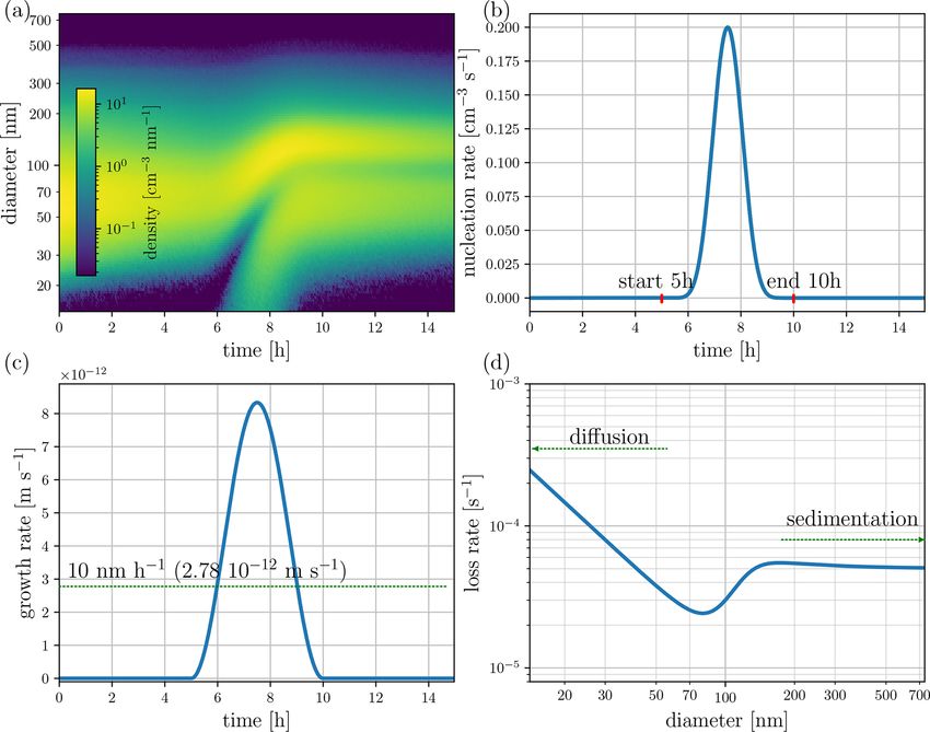
3718 M. Ozon et al.: Retrieval of process rate parameters in the GDE for aerosols
that is, Nik = i n(dp , tk )ddp , and a vector consisting of par-
R
uncertainties. We also model the process rate parameters as
discrete-time stochastic processes. This formulation allows ticle concentrations in all Q bins at time tk by N k , that
us to express the following questions in the Bayesian frame- is, N k = [N1k , . . ., NQ k ]T . We discretize the condensation and
work (Gelb, 1974):
deposition rates accordingly, and write g k = [g1k , . . ., gQ k ]T ,
– What are the expected values of n(dp , tk ), g(dp , tk ), λk = [λk1 , . . ., λkQ ]T . Further, the nucleation J is discretized
λ(dp , tk ) and J (tk ) at each time tk given a set of mea- with respect to time: J k denotes the nucleation rate at time
surements Y` = {y 1 , . . ., y ` } corresponding to discrete tk .
times t1 , . . ., t` ? Using Euler’s method for time integration and first-order
– How large are the uncertainties of the estimated quanti- upwind differencing for the condensation terms, we get the
ties? discrete-time evolution model for the particle number con-
centrations in bins i (Korhonen et al., 2004):
The state estimation problems are referred to as prediction, ! !
filtering and smoothing depending on whether ` < k, ` = k or k+1 k k k g1k
` > k, respectively. While filtering is a suitable choice for on- N1 = N1 + 1t J − + λ1 N1k + C1 (N k ) (5)
1d1
line monitoring and control problems, smoothing is usually ! !
k
a preferable choice when estimates are not needed online; k+1 k k
gi−1 k gik
Ni = Ni + 1t N − + λi Nik
the smoother estimates also utilize the future observations 1di−1 i−1 1di
y k+1 , . . ., y ` for the estimate corresponding to time tk .
The latter question refers to posterior uncertainties – that + Ci (N k ), (6)
is, uncertainties of the quantities given the measurements Y` . for all 1 < i ≤ Q, 1 ≤ k ≤ T,
In the Bayesian framework, these uncertainties can be quanti-
where Ci (N k ) is a nonlinear coagulation term; for details,
fied by computing, for example, posterior variances and cred-
see Lehtinen and Zachariah (2001). Here, the choice for ap-
ible intervals of the parameters.
proximating the derivative in the growth term in the dis-
In the simplest special case, where the evolution model
cretization of the GDE is made, assuming that the parti-
and observation model are linear with respect to all pa-
cle growth rate is positive. The modification to cases where
rameters and all error terms are additive and Gaussian, the
the aerosols evaporate, i.e., where growth rate is negative, is
Bayesian filtering and smoothing problems can be solved by
straightforward. Such a time discretization scheme can be-
Kalman filter and Kalman smoother recursions, respectively
come unstable; however, it is possible to apply a different
(Kalman, 1960; Gelb, 1974). In general cases, where models
method, e.g., implicit Euler or Crank–Nicholson (Trangen-
are nonlinear or non-Gaussian, only approximate solutions
stein, 2013). Equations (5) and (6) can be written equiva-
are available. In principle, the best approximations of the
lently in vector form as
posterior estimates are obtained with sequential Monte Carlo
methods, known as particle filters/smoothers (Särkkä, 2013).
N k+1 = A g k , λk N k + s J k + C β, N k . (7)
However, these methods are limited to small dimensional
cases, because of the high computational burden. Compu-
Here, A = A(g k , λk ) is a sparse matrix consisting of ele-
tationally more efficient approximations include ensemble,
ments Aij :
unscented and extended Kalman filters/smoothers (Särkkä,
2013). In this paper, we choose the extended Kalman filter
k
1 − 1t k gi + λi
i=j
(EKF) and fixed interval Kalman smoother (FIKS), but we
1di
note that the other filters and smoothers developed for nonlin- Aij (g k , λk ) = gk (8)
ear state estimation are applicable as well. In the next section,
1t k 1di−1
i−1
i = j +1 > 1
0 otherwise,
the feasibility of the EKF and FIKS for the GDE parameter
estimation problem will be tested numerically.
s = s(J k ) ∈ RQ is a vector of the form s(J k ) =
2.1 Evolution model [1t k J k , 0, . . ., 0]T , and the nonlinear term C(β, N k ) is
defined accordingly.
2.1.1 Discretized, stochastic GDE Finally, we complement the discretized GDE with a
stochastic term k ∈ RQ to account for modeling errors
To approximate the GDE (1) numerically, we partition the caused by factors such as discretization and uncertainties of
particle size variable dp into Q intervals (or bins) i of the boundary conditions, and we write
widths 1di , i = 1, . . ., Q. The discrete instants in time in
the temporal discretization are denoted by tk , k = 1, . . ., T , N k+1 = f N k + k , (9)
and the differences between consecutive times are denoted
by 1t k = tk+1 − tk . We denote the number concentration of where f : RQ → RQ is of the form f (N k ) = A(g k , λk )N k +
particles corresponding to the ith bin at time tk by Nik – s(J k ) + C(β, N k ). In this paper, the stochastic state noise
Geosci. Model Dev., 14, 3715–3739, 2021 https://doi.org/10.5194/gmd-14-3715-2021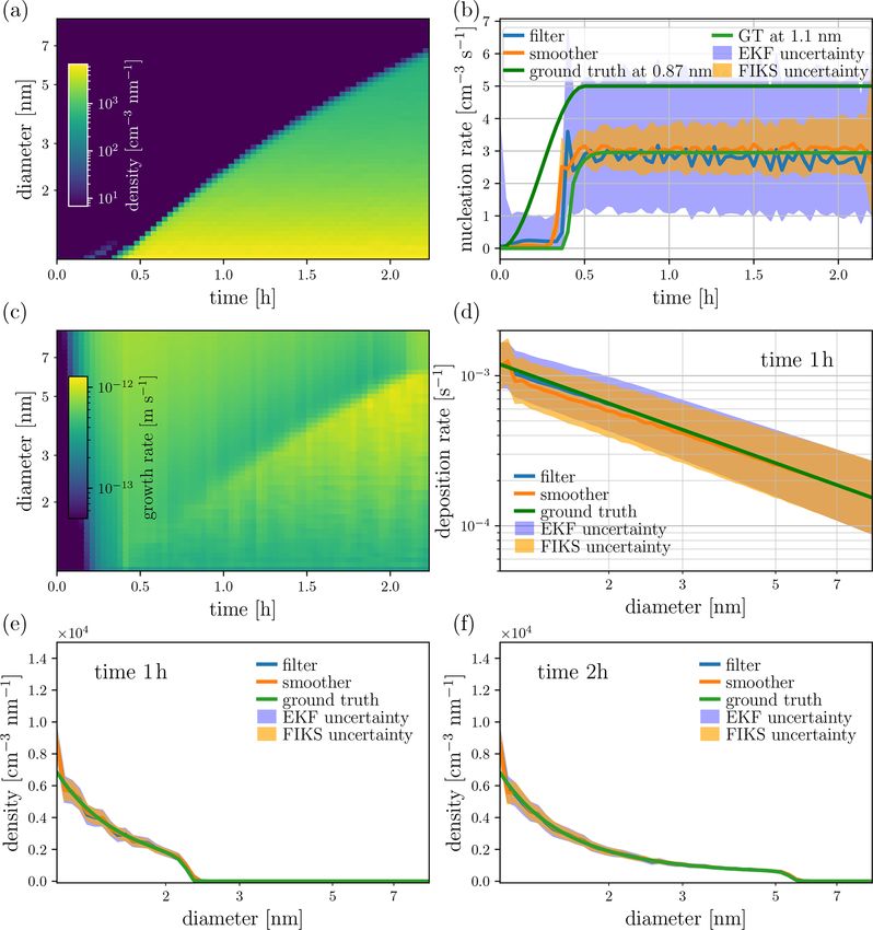
M. Ozon et al.: Retrieval of process rate parameters in the GDE for aerosols 3719
term k is modeled as Gaussian, k ∼ N (0, 0 ), where 0 is one to test the model’s feasibility against the driving noise
the covariance matrix of k . Equation (9) forms a discretized, distribution (variances) (Gelb, 1974). In the next section, we
stochastic evolution model for the particle number concentra- test the state estimation based on the above models in cases
tion N . where the true evolution of the quantities is not of the form
of Markov models.
2.1.2 Models for the parameters of the GDE
2.1.3 Augmented evolution model for n, g, λ and J
All the unknown parameters of the GDE (g, λ and J ) are
known to be nonnegative. For this reason, we reparametrize To complete the evolution model, we define an augmented
these quantities by writing gik = Pg (ξg,i
k ), λk = P (ξ k ) and
i λ λ,i state variable Xk ,
k k
J = PJ (ξJ ), where ξg,i , ξλ,i and ξJ are the (unconstrained) k
N
parameters, and mappings Pg , Pλ , PJ have the form of a so- ξ kg
called softplus function (Dugas et al., 2001) Pϕ : R → R+ : k
X = (13)
ξk ,
λ
1 k
ξ kJ
Pϕ (ξϕk ) = log 1 + eαξϕ . (10)
α
and combine the evolution models written in Sects. 2.1.1 and
Note that this parameterization only constrains the param-
2.1.2, yielding
eter from below, but if an upper boundary is known, the
function in Eq. (10) could be changed in favor of, for ex- k+1
N
ample, a logistic function which allows for both constraints ξ k+1
g
from below and from above. We denote the vectors consist- =
ξ k+1
ing of all condensation and deposition parameters at time tk λ
ξ k+1
by ξ kg = [ξg,1
k , . . ., ξ k ]T and ξ k = [ξ k , . . ., ξ k ]T , respec-
g,Q λ λ,1 λ,Q
J
Nk
tively. A(Pg (ξ kg,i ), Pλ (ξ kλ,i )) 0 0 0
As the process rates g, λ and J in the GDE are time- 0 9g 0 0
ξ kg
×
0 0 9λ 0 ξ kλ
varying, the state estimation requires one to model their time
dependence. In this paper, we model ξg,i , ξλ,i and ξJ as either 0 0 0 9J ξ kJ
first-order Markov processes,
k
s(PJ (ξJk )) C(β, N k )
ξ k+1 = 9 ϕ ξ kϕ + ηkϕ , (11) 0 0 ηkg
+ + + (14)
ϕ
0 0 ηkλ
where 9 ϕ is a diagonal matrix 9 ϕ = rϕ I, and 0 < rϕ < 1, or 0 0 ηk J
as second-order Markov processes,
or
ξ k+2
ϕ = 9 1ϕ ξ k+1
ϕ + 9 2ϕ ξ kϕ + ηkϕ , (12)
Xk+1 = F Xk + w k . (15)
with 9 1ϕ = rϕ1 I and 9 2ϕ = rϕ2 I. In both models, ηkϕ stands for
Gaussian noise ηkϕ ∼ N (0, 0 ηϕk ). To simplify the following This is the evolution model for the augmented state variable
description, we assume all the models to be of the form Xk , which includes not only the number concentrations of
shown in Eq. (11), but we note that the extension to second- the size sections but also the unknown process rates. Next,
order models is straightforward: higher-order Markov mod- we write the observation model in terms of Xk , and then,
els can be converted into the form of first-order Markov mod- in Sect. 2.3, we apply Bayesian state estimation to infer Xk ,
els by augmenting the state variables corresponding to more k = 1, . . ., K based on sequential SMPS measurements.
than one time instant into a single vector. The second-order
2.2 Observation model
models are suitable for some of the quantities in GDE, be-
cause they imply temporal smoothness of those processes An SMPS consists of a differential mobility analyzer
(Kaipio and Somersalo, 2006). The specific choices of the (DMA), which classifies charged particles based on their mo-
state models and their parameters are discussed in Sect. 3 bility in an electric field, and a condensation particle counter
and specified in Appendix B. (CPC) where the classified particles are grown to sizes de-
The evolution models, such as Eqs. (11) and (12) can be tectable, for example, optically. All particle counters provide
argued to be unrealistic, as they are not based on physics. The only discrete, indirect and noisy data on the particle size dis-
understanding, however, is that if the (co)variances of the tributions. Mathematically, each channel in a particle counter
driving noise processes ηkϕ are set high enough, such mod- gives data that corresponds to a convolution/projection of the
els are feasible in the sense that the actual ξ k+1
ϕ − 9 ϕ ξ kϕ are particle size distribution onto a space spanned by device-
well supported by the modeled distribution of ηkϕ . System- specific kernel functions; moreover, the counter data are cor-
atic (state-space identification) approaches exist that allow rupted by Poisson distributed noise.
https://doi.org/10.5194/gmd-14-3715-2021 Geosci. Model Dev., 14, 3715–3739, 2021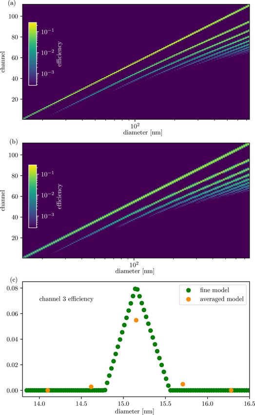
3720                                                  M. Ozon et al.: Retrieval of process rate parameters in the GDE for aerosols

2.2.1       SMPS transfer function                                          Finally, the model (Eq. 19) can be written in terms of the
                                                                         state variable Xk defined in Eq. (13),
The output of each DMA is the detected number concentra-
tion in a size class; in channel i corresponding to a discrete           y k = HXk + ek ,                                            (20)
time index k, it is of the form
                                                                         where H is a block matrix of the form H = [H̄, 0, 0, 0].
                 t0Z
                   +k1t         Z
        1
zik =                     φa (t) 9i (dp )n(dp , t)ddp dt,        (16)    2.3   State estimation
        V
            t0 +(k−1)1t         ωi
                                                                         The nonlinear evolution model (Eq. 15) and the linear obser-
where 9i (dp ) is a time-invariant kernel function; ωi is the            vation model (Eq. 20) form a system
support of 9i (dp ) – that is, the set of points where 9i (dp )
is nonzero; t0 is the initial time; and 1t is the duration of            X k+1 = F Xk + w k                                      (21)
counting particles in the CPC for a single channel. Further,
                                                                         y k = HXk + ek ,                                            (22)
V is the volume of the aerosol sample that passes through
the CPC counter with a detector–sample       flow rate φa (t) in
                                       R t +k1t                          referred to as the state-space representation. The system
the period of time 1t – that is, V = t00+(k−1)1t φa (t)dt.               is stochastic due to the state noise and observation noise
                                                                         processes, wk and ek , respectively. In addition, we model
2.2.2       CPC counting model
                                                                         the initial state X0 as a Gaussian random variable X 0 ∼
The measurement data of the ith channel of an SMPS, yik ,                N (X0|0 , 0 0|0 ). Given this model, we can state the Bayesian
consist of Poisson-distributed counts given by the CPC:                  filtering and smoothing problems as follows: form the con-
                                                                         ditional probability density of the random variable X k , given
        ỹik                                                           the sequence of measurements Y` = {y 1 , . . ., y ` }. In the ex-
yik =        ,    with ỹik ∼ Poisson V zik ,                    (17)    tended Kalman filter and smoother, these probability densi-
        V
                                                                         ties π(Xk |Y` ), are approximated by Gaussian densities – that
where V ' 1tφa (t0 + k1t) is the volume of sample used in                is,
the CPC for counting. In the numerical studies of this paper,
we use this model when simulating the measurement data. In               π(X k |Y` ) ≈ N (Xk|` , 0 k|` ),                            (23)
state estimation, however, we approximate the Poisson dis-
tributed observations as Gaussian:                                       where Xk|` and 0 k|` are approximations of the respec-
                                                                       tive conditional expectation and covariance of Xk given Y`
yik ∼ N zik , γi ,                                       (18)            (Gelb, 1974).
                                                                            Kalman filtering gives online estimates π(Xk |Yk ) based
where γi is the approximate variance of the noise. In this               on the data set from the beginning up to the present time k
paper, we use the same approximation as in Voutilainen et al.            – that is, ` = k, whereas in smoothing ` > k. In the FIKS, in
                               yk
(2000) and write γik = Vi .                                              particular, ` = K, where K is the index of the final time step.
   By discretizing the SMPS model (Eq. 16) and using the                 In other words, the FIKS estimate π(X k |YK ) at each time
above Gaussian approximation of the noise, we write an ob-               k is based on the entire data set from the beginning to the
servation model of the form                                              end of measurements. The EKF and FIKS estimates (approx-
                                                                         imate expectations Xk|` and covariances 0 k|` ) are given by
y k = H̄N k + ẽk + ιk ,                                         (19)    the following forward and backward iterations (Gelb, 1974):
where y k = [y1k , . . ., yMk ]T , H̄ is an observation matrix and ẽk

is the Gaussian observation noise ẽk ∼ N (0, 0 kẽ ). Here, the
covariance of the observation noise is of the diagonal form
0 ke = diag(γ1k , . . ., γM
                          k ). The additional noise term, ιk is in-

cluded in Eq. (19) in order to account for errors caused by the
discretization of the measurement operator in Eq. (16). Here,
ιk is simply approximated as being Gaussian distributed with
zero-mean ιk ∼ N (0, 0 kι ) whose components are calculated
as mutually independent; hence, the covariance matrix 0 kι
is of diagonal form. Furthermore, the approximation error
term ιk is assumed to be independent of the counting noise
ẽk ; thus, the total error ek = ẽk +ιk ∼ N (0, 0 ke ), where 0 ke =
0 kẽ +0 kι . For a more rigorous approach to handling modeling
errors, we refer to the book by Kaipio and Somersalo (2006).

Geosci. Model Dev., 14, 3715–3739, 2021                                                    https://doi.org/10.5194/gmd-14-3715-2021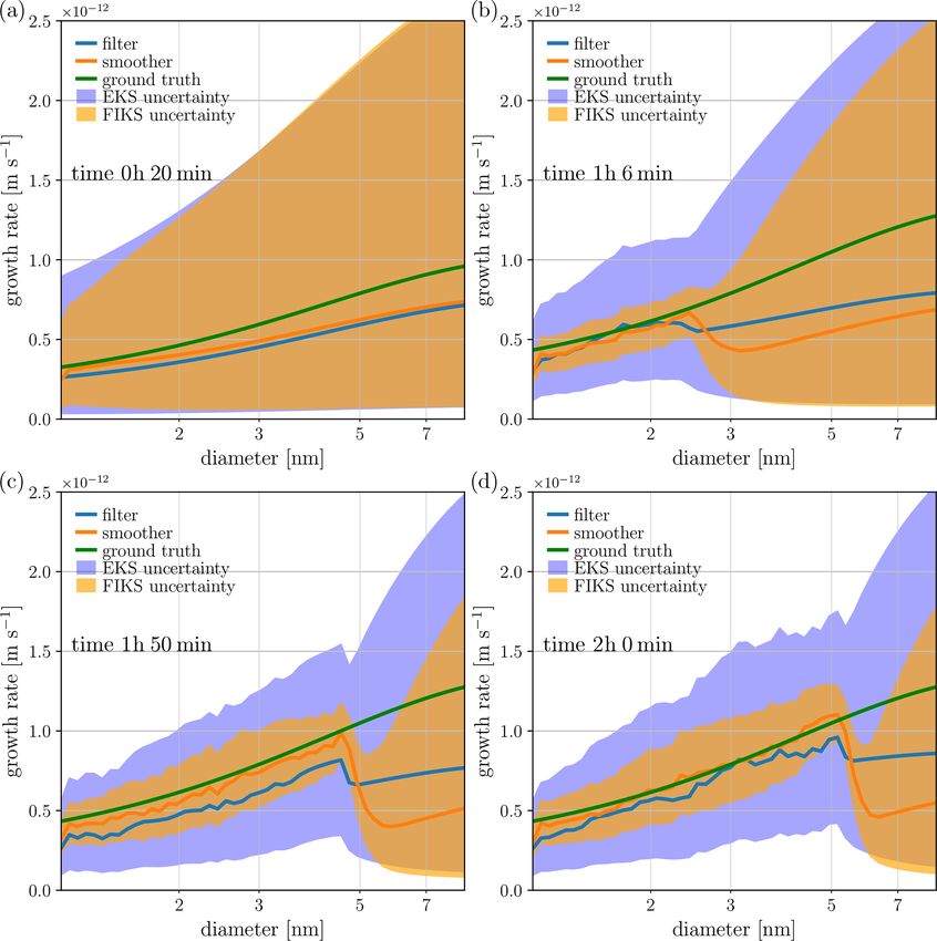
M. Ozon et al.: Retrieval of process rate parameters in the GDE for aerosols                                                 3721

                                                                  time. Further, the nucleation rate J is a time-dependent, con-
                                                                  tinuous function which represents an NE in a time interval
                                                                  [t0 = 5 h, t1 = 10 h] and is zero in all other instants within
                                                                  the period of interest [0, 15 h]. As noted above, the coagula-
                                                                  tion kernel is known, yet the coarse discretization also causes
                                                                  error in this term. The detailed forms of the process rates are
                                                                  shown in Table A1 (Appendix A).
                                                                     When simulating the evolution of the particle distribu-
                                                                  tion, the particle diameter dp ∈ [13.85 nm, 1000.0 nm] is
   In Algorithms 1 and 2, ∂F k denotes the Jacobian matrix of     discretized into Q = 2500 logarithmically distributed bins.
the nonlinear mapping F at point Xk|k . Note that the FIKS        Such a high size resolution is chosen in order to avoid numer-
is based on a backward recursion, which starts from the filter    ical diffusion effects and to obtain a good approximation of
estimate corresponding to final state: XK|K , 0 K|K .             the particle size density. The time step 1t k in the explicit Eu-
                                                                  ler time integration scheme is chosen based on the Courant–
                                                                  Friedrichs–Lewy condition (Courant et al., 1928; Dullemond
3     Numerical simulations                                       and Dominik, 2005):

                                                                                         1
In this section, the feasibility of the proposed estimation       0 < 1kt <                         .                       (24)
scheme is tested with numerical studies, where the aerosol                              gik
                                                                              max       1di   + λi
particle evolution is simulated by numerical approximations                    i
of the GDE corresponding to a set of process rates, and where
synthetic SMPS data are computed by numerical modeling of         The CFL criterion is applied in order to keep the time inte-
the DMA and generating the Poisson-distributed CPC data.          gration stable with respect to condensational growth and loss.
Two type of events are considered: in cases 1 and 2, the evo-     The coagulation rates are not considered here because coagu-
lution of the aerosol size distribution is governed by a nu-      lation is actually a dampening mechanism that stabilizes time
cleation event (NE) and the subsequent growth of the nucle-       integration. The nucleation, growth and loss rates as well as
ation mode in a background of existing aerosols; in cases         the resulting particle size density evolution for the NE cases
3 and 4, new particles are formed in a continuous nucle-          are illustrated in Fig. 1.
ation process and their further evolution is controlled by con-      As explained in Sect. 2.2, the measurements consist of
densational growth and deposition, so that the size distribu-     simulated counts modeling CPC combined with DMA. The
tion approaches a steady state (SS). In all cases, the particle   model for the kernel functions 9i (dp ) corresponds to an
growth is dominated by condensation, and the loss of parti-       SMPS 3936 device, and it accounts for the most relevant
cles (caused by wall deposition, sedimentation, dilution, etc.)   effects (Millikan, 1923; Stolzenburg, 1989; Flagan, 1998;
depends linearly on the size distribution function. Further,      McMurry, 2000; Boisdron and Brock, 1970; Wiedensohler,
the coagulation kernel is chosen to have the form given in        1988). We skip the details here, and only visualize the ker-
the book by Seinfeld and Pandis (2016). In these numeri-          nels, by plotting the size-distribution transfer function, or the
cal studies, cases 1 and 2 (NE) qualitatively represent a typi-   observation matrix H̄, as a color map (Fig. 2a).
cal particle formation event in the atmosphere (e.g., Hyytiälä       We simulate the synthetic CPC measurement yik corre-
Maso et al., 2005), whereas cases 3 and 4 (SS) represent par-     sponding to each CPC channel i at each time k by draw-
ticle formation and growth in a chamber experiment (e.g.,         ing samples from a Poisson distribution, given in Eq. (17)
CLOUD Lehtipalo et al., 2014).                                    with mean V zik . As the expectation of yik is zik and its
                                                                  variance is zik /V , the signal-to-noise ratio (SNR) of CPC
3.1     Cases 1 and 2: nucleation event (NE)                      data increases with V . In order to investigate the effect of
                                                                  SNR to the process rate estimates, we generate the Poisson-
3.1.1    NE: data simulation                                      distributed observations corresponding to two sample vol-
                                                                  umes: V = 90 cm3 (Case 1: NE, high SNR) and V = 0.9 cm3
In the numerical simulation study, the temporally evolving        (Case 2: NE, low SNR). In Case 1, the range of SNR was
particle size distribution is synthetically generated using the   [0, 6426]; in Case 2 it was [0, 64.26].
(deterministic) discretized GDE model described by Eqs. (5)
and (6) with predefined process rates g, λ, β and J . In the      3.1.2   NE: parameter estimation
estimation, however, g, λ and J are, of course, not known.
   In the NE case, the process rates g, λ and J are chosen        In this section, we briefly describe the assumptions made
to have the following properties: the condensational growth       when constructing the models used for computing the state
rate g is independent of the particle size but depends on time,   estimates in the NE cases. The exact forms of the models as
whereas the loss rate λ depends on particle size but not on       well as choices of parameters are listed in Appendix B.

https://doi.org/10.5194/gmd-14-3715-2021                                                Geosci. Model Dev., 14, 3715–3739, 2021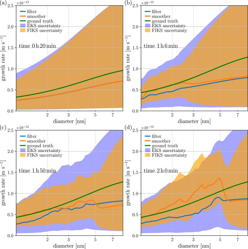
3722                                             M. Ozon et al.: Retrieval of process rate parameters in the GDE for aerosols

Figure 1. Cases 1 and 2 – a nucleation event, showing true (simulated) processes: (a) particle size density (measurement), (b) nucleation
rate, (c) growth rate and (d) loss rate.

   For the evolution models used in state estimation, the par-         the stochastic terms is a crucial part of the state-space model.
ticle size range [14.1 nm, 736.5 nm] is divided into 111 bins –        However, the state estimates are not extremely sensitive to
that is, the size range is narrower and the discretization is sig-     these choices; choosing parameters that are of the right order
nificantly coarser than when simulating the data. The GDE-             of magnitude is usually enough, and as the stochastic models
based, discrete stochastic state evolution model (Eq. 9) for           are written for physically relevant quantities, ballpark ranges
the particle number N is written as described in Sect. 2.1.1.          of the parameters are often available a priori.
The covariance matrix 0  of the stochastic term  k is chosen            The size-distribution transfer function corresponding to
to be of diagonal form.                                                the discretization of the particle size in estimation is illus-
   In this case study, we assume to know that the condensa-            trated in Fig. 2b. The approximate observation model is used
tion rate is time dependent but size independent. Moreover,            in order to avoid so-called inverse crime, which refers to the
both the condensation and nucleation rates are assumed to              use of unrealistically accurate models in the inversion of sim-
be temporally smooth, and we model them as second-order                ulated data. A comparison between the true transfer function
stochastic processes (Eq. 12). The loss factor λ is assumed to         and the approximated one used in the estimation – mean over
be a smooth function of the particle size. Further, we write a         each discretization bins – is depicted in Fig. 2c for the third
first-order Markov model (Eq. 11) for its temporal variation           channel. Furthermore, as noted in Sect. 2.2, instead of us-
– that is, although the true loss factor is time invariant, we do      ing the Poisson model for the measurements, the observation
not assume to know this property in state estimation. This is          noise is approximated as additive and Gaussian. This choice
done to study the stability of the estimation scheme: although         is made for computational convenience, as it allows for the
the deposition loss is modeled as varying with time, the esti-         direct applications of EKF and FIKS into the state-space sys-
mation should yield essentially time-invariant estimates.              tem.
   The covariance of the initial state, 0 0|0 , is chosen to be           The extended Kalman filter and smoother estimates are
diagonal; this signifies that the elements of X0 are mutually          computed using Algorithms 1 and 2, respectively. From
independent. Moreover, the variances of X0 are chosen to               the resulting state estimates Xk|` , ` = k, K the approximate
be relatively large in comparison with the variances of the            posterior expectations of the processes are computed using
state noise vector  k ; this indicates a high uncertainty of the      the models gik = Pg (ξg,ik ), λk = P (ξ k ) and J k = P (ξ k )
                                                                                                      i      λ λ,i                J J
initial state. We note that the selection of the parameters in         (see Sects. 2.1.2 and 2.1.3). We also compute approximate

Geosci. Model Dev., 14, 3715–3739, 2021                                                 https://doi.org/10.5194/gmd-14-3715-2021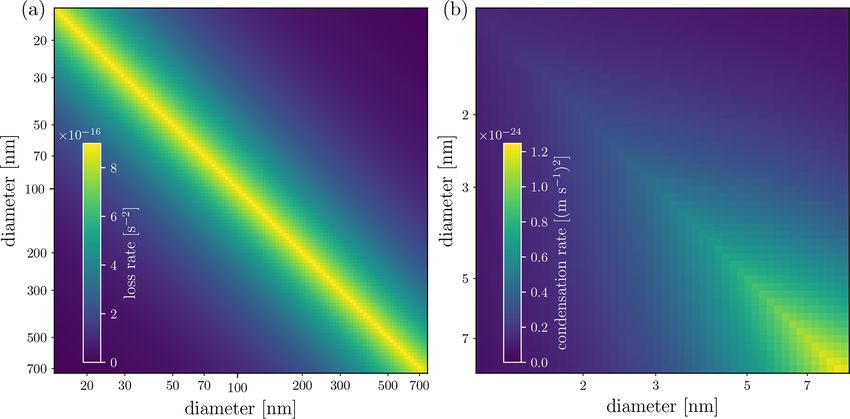
M. Ozon et al.: Retrieval of process rate parameters in the GDE for aerosols 3723
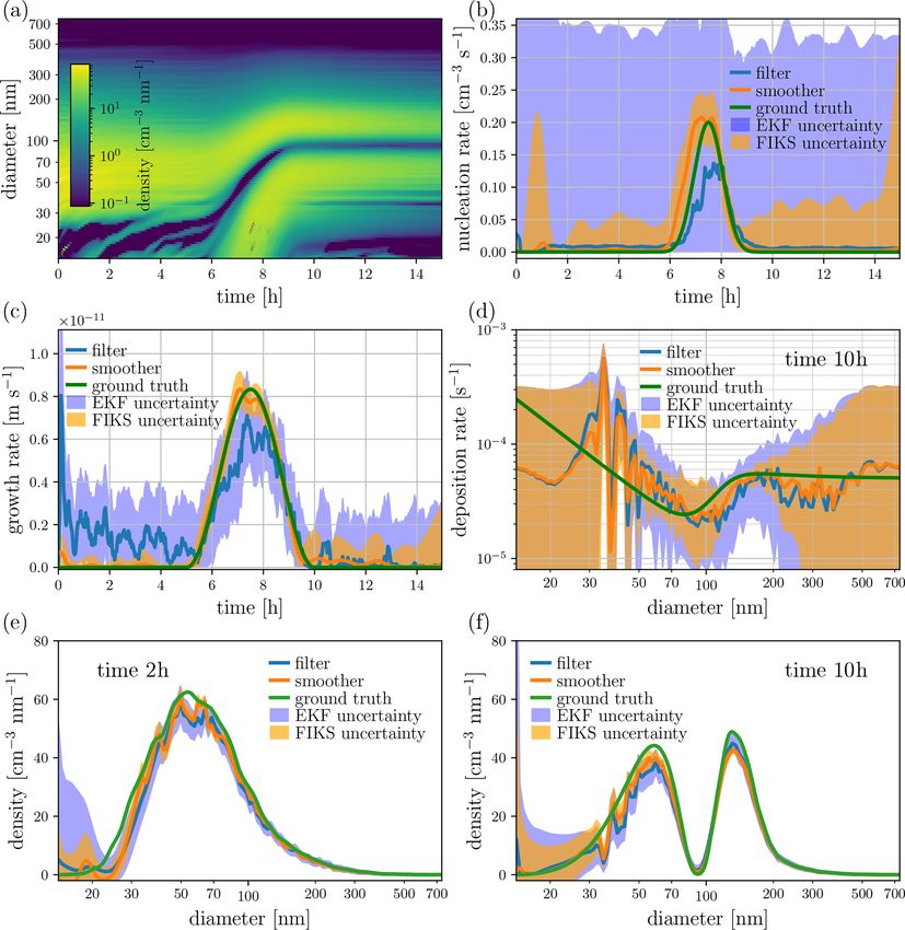
3.1.3 NE: results and discussion
The results of Case 1 (NE, high SNR) are illustrated in Fig. 3.
The figure shows the Kalman smoother estimates for the par-
ticle size density, and the EKF and FIKS estimates for the
growth, apparent particle formation and loss rates as well as
1N
for two instantaneous particle size densities ( 1d p
at 2 and
10 h). The loss rate estimates correspond to time 10 h. For
the process rates and for the instantaneous size densities, the
figure also shows the EKF- and FIKS-based posterior error
intervals – representing the uncertainty of the estimates – as
well as the true values of the corresponding quantities.
The estimated particle size density (Fig. 3a) is in rather
good correspondence with the true size density (Fig. 1a).
However, the size density estimates corresponding to times 2
and 10 h (Fig. 3e and f, respectively) show that the peak val-
ues of the size density are somewhat underestimated by both
EKF and FIKS. Moreover, in these instants, the true values of
the size density are partly outside the approximate posterior
error intervals. Yet the 68 % posterior error intervals do not
necessarily need to contain the true values, and the error in-
tervals seem to be slightly too narrow. This underestimation
of the uncertainty is due to the linearizations/Gaussian ap-
proximation behind EKF and FIKS, as shown by Huttunen
et al. (2018), and the rather simple approximations of the er-
ror in the evolution and the measurement models – under-
estimating the covariance in the models. The errors caused
by model approximations become more influential with de-
creasing mean noise level – the remedy for such errors could
be the Bayesian approximation error method (Kaipio and
Somersalo, 2006); however, this is out of the scope of this
paper.
For the process rates, the approximate posterior means
Figure 2. The size distribution transfer functions for (a) simulating given by both EKF and FIKS are relatively close to the true
the measurement data, and (b) the observation model used in state values (Fig. 3b–d). Overall, the FIKS estimates for the pro-
estimation. In the images, the horizontal axis corresponds to the size cess rate parameters are more accurate than the EKF esti-
of the particle entering the device, and the vertical axis represents mates – this is an expected result because FIKS utilizes the
the channels of the SMPS. The colors represent the values of the entire data set up to the end of the process, whereas EKF only
efficiency with which a given particle size will be classified in a
uses data up to time t when estimating the variables at time
given bin in the particle sizer.
t.
The filter and smoother also show differences in the pos-
68 % credible intervals terior error intervals of the process rate parameters: the error
q of the estimates, by mapping the val- intervals given by EKF are systematically wider than those
ues E(ξ∗,ik |Y` ) ± var(ξ k |Y` ), to the corresponding pro-
∗,i given by FIKS. This is again an expected result because the
cess rate spaces. Note, however, that due to the lineariza- use of the future data (FIKS) should reduce the uncertainty in
tions/Gaussian approximation behind EKF, these approxi- the estimated quantities. Furthermore, in almost all instants
mate intervals do not necessarily represent the ranges where in time, the process rate parameters (especially growth and
the true parameter value lies; these are the ranges within apparent particle formation rates) are within the posterior er-
which the true value most likely lies with an 0.68 probabil- ror intervals. This is a desired result, as it indicates that these
ity. In the following, we refer to these approximate credible approximate credible intervals give realistic measures of the
intervals as“posterior error intervals”. estimate uncertainties in these cases.
The loss rate estimate uncertainty depends strongly on the
particle size: the posterior error intervals are wide in the low-
est and highest size ranges and rather narrow elsewhere. The
high uncertainty of the loss factor at the high particle size
https://doi.org/10.5194/gmd-14-3715-2021 Geosci. Model Dev., 14, 3715–3739, 2021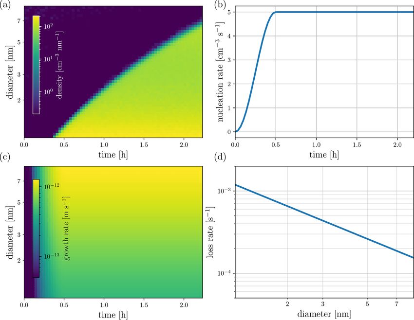
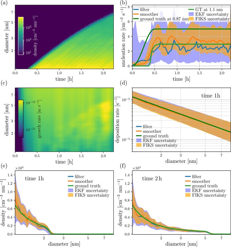
3724                                               M. Ozon et al.: Retrieval of process rate parameters in the GDE for aerosols

Figure 3. Case 1 – NE and high SNR. State estimates for the particle size density (a, e, f), nucleation rate (b), growth rate (c) and loss rate
(d). The image in plot (a) depicts the approximate posterior expectation for the entire time-evolution of the particle size density given by
FIKS, whereas plots (e) and (f) illustrate the EKF and FIKS estimates corresponding to times 2 and 10 h, respectively. In plots (b)–(f), the
blue and orange lines represent the approximate posterior expectations for EKF and FIKS, respectively, and the areas shaded with light blue
and orange are the respective posterior error intervals. The true values of the corresponding quantities are drawn with a green line.

range dp > 400 nm is caused by the lack of data – in this size               In Case 1, the SNR is high, and – apart from the afore-
range, the particle density is nearly zero at all times; conse-           mentioned exceptions – the estimate uncertainty is very low.
quently, the SMPS data do not provide information on the                  Figure 4 shows the results of Case 2, where the SNR is signif-
loss factor. In the lowest size range, the width of the credible          icantly lower. As expected, the process rate estimates become
interval also depends on time. From time t = 9 h, when the                less accurate than in Case 1. However, the change in the accu-
nucleation event is practically over, the particle size density           racy is quite small, especially for FIKS – demonstrating that
in the lowest size range is almost zero, again resulting in high          the Kalman smoother estimates tolerate measurement noise
uncertainty in the loss factor estimate. The loss rate estimate           rather well. As expected, the posterior error intervals of all
and posterior error interval resulting from the FIKS are vir-             estimated quantities are clearly wider than in the case of high
tually time invariant, even though those from the EKF show                SNR – this is a result of increased uncertainty in the parti-
a strong time dependence.                                                 cle counter observations. Both EKF and FIKS lead to safe

Geosci. Model Dev., 14, 3715–3739, 2021                                                     https://doi.org/10.5194/gmd-14-3715-2021
M. Ozon et al.: Retrieval of process rate parameters in the GDE for aerosols                                                            3725

Figure 4. Case 2 – NE and low SNR. State estimates for the particle size density (a, e, f), nucleation rate (b), growth rate (c) and loss rate
(d). The image in plot (a) depicts the approximate posterior expectation for the entire time-evolution of the particle size density given by
FIKS, whereas plots (e) and (f) illustrate the EKF and FIKS estimates corresponding to times 2 and 10 h, respectively. In plots (b)–(f), the
blue and orange lines represent the approximate posterior expectations for EKF and FIKS, respectively, and the areas shaded with light blue
and orange are the respective posterior error intervals. The true values of the corresponding quantities are drawn with a green line.

posterior error intervals for the process rate parameters, and           stability of Eqs. (5) and (6) which are corrected during the
FIKS again gives clearly narrower posterior error intervals              estimation by the assimilation of the data. However, while
than EKF. The true values of the process rate parameters are             the data in Case 1 allow for the estimates to be neatly recti-
once again within the posterior error intervals, further con-            fied, the data in Case 2 cannot completely make up for the
firming the feasibility of Bayesian state estimation for quan-           instability. Note that the tolerance with respect to such mod-
tifying the uncertainties of the process rates.                          eling errors (e.g., discretization) can be further improved by
   One may notice the appearance of spurious oscillations in             so-called approximation error analysis (Huttunen and Kai-
the size distribution at low sizes during the particle formation         pio, 2007).
event in Case 2 (Fig. 4a), which were completely smoothed
out in Case 1 (Fig. 3a). These oscillations are due to the in-

https://doi.org/10.5194/gmd-14-3715-2021                                                     Geosci. Model Dev., 14, 3715–3739, 2021
3726                                             M. Ozon et al.: Retrieval of process rate parameters in the GDE for aerosols

Figure 5. Cases 3 and 4 – steady-state system, showing true (simulated) processes: (a) particle size density (measurement), (b) nucleation
rate, (c) growth rate and (d) wall loss rate.

3.2     Cases 3 and 4: steady state (SS)                               simulated by generating the Poisson-distributed observations
                                                                       corresponding to two sample volumes: V = 200 cm3 (Case
3.2.1    SS: data simulation and parameter estimation                  3: SS, high SNR) and V = 2 cm3 (Case 4: SS, low SNR). In
                                                                       Case 3, the range of SNR was [0, 4440]; in Case 4 it was
In the SS simulations in this paper, the condensation rate             [0, 44.4].
is both size dependent and time dependent, and the wall                   In the state space, the lower end of the size discretization
loss rate is time invariant but depends on size. Both the nu-          bin (i.e., 1 in Sect. 2.1.1) is centered at 1.1 nm (its lower
cleation and condensation rates start from zero and grow               boundary is about 1.08 nm). Many potential bins would sep-
within the first 30 min until they reach their stationary val-         arate the critical size dp∗ = 0.87 nm from the lower end of
ues. In such a case, the new particle formation and conden-
                                                                       the state space dpmin = 1.08 nm. The reason that we are not
sational growth are compensated for by wall losses, lead-
ing to the number concentration function to reach a steady             setting dpmin = dp∗ is because, with the current technology, it
state. The simulated process rates and the particle size den-          is not realistic to assume that we can acquire reliable data
sity are illustrated in Fig. 5. Here, the size range of particles      down to the critical size. Note that it is possible, however, to
is [0.87 nm, 10.00 nm], and it is discretized into Q = 1731            extend the model down to the critical size in order to esti-
logarithmically distributed bins. Note that the value dp∗ =            mate the true nucleation rate – provided that the GDE is still
0.87 nm is most certainly below any physically relevant crit-          valid for such small particles. However, without measure-
ical sizes; however, from a simulation stand point, any size           ment from the lower end of the spectrum, the uncertainty will
range could have been utilized to simulate a similar chamber           overwhelm the estimates, rendering them non-informative.
experiment, only the values of the parameters would require            This extension is outside of the scope of this paper.
adjustments.                                                              The time evolution of the apparent particle formation and
   The synthetic SMPS data are simulated similarly to cases 1          growth rates are modeled as second-order Markov processes
and 2. Again, two cases corresponding to different SNRs are            (Eq. 12), whereas the wall loss rates are modeled as first-

Geosci. Model Dev., 14, 3715–3739, 2021                                                  https://doi.org/10.5194/gmd-14-3715-2021
M. Ozon et al.: Retrieval of process rate parameters in the GDE for aerosols 3727
Figure 6. Case 3 – SS, high SNR. State estimates for the particle size density (a, e, f), nucleation rate (b), growth rate (c) and wall loss rate (d).
The images in plots (a) and (c) depict the approximate, FIKS-based posterior expectations for the entire time-evolution of the corresponding
quantities. Plots (e) and (f) illustrate the EKF and FIKS estimates for the particle size density corresponding to times 1 and 2 h, respectively.
In plots (b) and (d–f), the blue and orange lines represent the approximate posterior expectations for EKF and FIKS, respectively, and the
areas shaded with light blue and orange are the respective posterior error intervals. The true values of the corresponding quantities are drawn
with a green line.
order Markov processes (Eq. 11). The growth and wall loss 3.2.2 SS: results and discussion
rates are assumed to be smooth with respect to size; hence,
the state noises in the corresponding evolution models are
modeled as correlated. For details of the model choices, we Figure 6 illustrates the estimates of the particle size density
refer to Appendix B. and process rates in the case of high SNR (Case 3). For the
particle size density and condensation rate, the respective im-
ages in Fig. 6a and c show the approximate FIKS-based pos-
terior means of those time- and size-dependent variables. For
the nucleation rate as well as for the instantaneous wall loss
https://doi.org/10.5194/gmd-14-3715-2021 Geosci. Model Dev., 14, 3715–3739, 20213728 M. Ozon et al.: Retrieval of process rate parameters in the GDE for aerosols Figure 7. Case 3 – SS and high SNR. Condensational growth rate estimates corresponding to four instants in time. The blue and orange lines represent the approximate posterior expectations for EKF and FIKS, respectively, and the areas shaded with light blue and orange are the respective posterior error intervals. The true growth rates are marked with green lines. rate and size densities, both the filter and smoother estimates are a major factor determining the accuracy of the estimates: (approximate posterior expectations and error intervals) are the higher the SNR, the better the estimate. While the true plotted. nucleation rate plotted in dark green takes place at 0.87 nm, In this case, the smoother estimate for the particle size den- in the state-space model, the diameter that corresponds to the sity is in very good correspondence with the true density (see apparent particle formation, plotted in light green, is about Fig. 5a). Further, the uncertainty estimates for the particle 1.08 nm (the lower end of the smallest size bin, geometrical size density are feasible: the true size density lies within the center at 1.1 nm). This difference between the model used for posterior error intervals given by EKF and FIKS. simulating the data and the model used in estimation causes The apparent particle formation rate is well estimated by the systematic error – underestimation of the nucleation rate. both the EKF and the FIKS; the true value lies within the Figure 6c shows a clear trend in the quality of the smoother posterior error intervals most of the time. Only at the onset of estimate for the condensational growth rate: at an early stage the appearance of particles into the measured size range does of the process (time ∼ 0.25 h), FIKS infers the growth rate the true value not lie within the uncertainty range, around reliably only in the smallest size classes (diameter ∼ 1 nm); t = 25 min. Similarly to the NE cases, the FIKS estimates are in the larger particle sizes, the growth rate is heavily under- less uncertain than those from the EKF, and the SNR levels estimated (see Fig. 5c). As time progresses, the growth rate Geosci. Model Dev., 14, 3715–3739, 2021 https://doi.org/10.5194/gmd-14-3715-2021
M. Ozon et al.: Retrieval of process rate parameters in the GDE for aerosols                                                              3729

Figure 8. Case 4 – SS and low SNR. State estimates for the particle size density (a, e, f), nucleation rate (b), growth rate (c) and wall
loss rate (d). The images in plots (a) and (c) depict the approximate, FIKS-based posterior expectations for the entire time-evolution of
the corresponding quantities. Plots (e) and (f) illustrate the EKF and FIKS estimates for the particle size density corresponding to times 1
and 2 h, respectively. In plots (b) and (d–f), the blue and orange lines represent the approximate posterior expectations for EKF and FIKS,
respectively, and the areas shaded with light blue and orange are the respective posterior error intervals. The true values of the corresponding
quantities are drawn with a green line.

estimates become gradually more reliable in larger and larger             follows accurately the propagating front of the number den-
size classes.                                                             sity in Fig. 6a. The reason for this property of the growth
   The gradual improvement in the growth rate estimates in                rate estimate is obvious: in the size classes where the par-
the larger size classes is a direct consequence of the propaga-           ticle number density is very low, the measurement data do
tion of the particle number density towards large size classes.           not carry information on the growth rate parameters. In the
Indeed, comparison of Fig. 6a and c reveals that the size class           beginning of the process, the particle number density is low
where FIKS catches the increase in the growth rate parame-                in all classes. When nucleation starts producing particles to
ter (light/yellow area in the condensation rate image Fig. 6c)            the smallest size class and these particles grow, the growth is

https://doi.org/10.5194/gmd-14-3715-2021                                                       Geosci. Model Dev., 14, 3715–3739, 2021
3730                                            M. Ozon et al.: Retrieval of process rate parameters in the GDE for aerosols

Figure 9. Case 4 – SS and low SNR. Condensational growth rate estimates corresponding to four instants in time. The blue and orange lines
represent the approximate posterior expectations for EKF and FIKS, respectively, and the areas shaded with light blue and orange are the
respective posterior error intervals. The true growth rates are marked with green lines.

sensed by the particle size analyzer measurements. When the            ing high uncertainty in the growth rate estimates in this size
particle sizes keep increasing due to condensation, the mea-           range. As time progresses, the size range of low uncertainty
surements corresponding to increasingly larger size classes            spreads towards large size classes. This result demonstrates
become sensitive to the process rate parameters.                       that Bayesian filtering and smoothing yield feasible poste-
   Figure 7 illustrates the EKF and FIKS estimates of the              rior error estimates – indicating high uncertainty in the size
growth rate corresponding to four instants in time. These              ranges where the posterior expectations are unreliable in this
plots confirm the above discussion on the growth rate es-              example.
timation: at time 1 h and 6 min, both the EKF- and FIKS-                  The EKF estimates of the growth rate in Fig. 7 show sim-
based posterior means underestimate the growth rate in the             ilar behavior to the FIKS estimates; the main differences are
large size classes (above ∼ 2.5 nm), and for the subsequent            that, as expected, the posterior means given by EKF are more
times, the EKF and especially FIKS estimates become reli-              biased than those in FIKS, and the posterior error intervals
able in gradually increasing size classes. Furthermore, Fig. 7         are generally wider than with FIKS.
shows a trend in the evolution of the posterior error inter-              Figures 8 and 9 show the results of Case 4 – SS and low
vals of the growth rate: at time 1 h and 6 min, the posterior          SNR data. The properties of the state estimates are very sim-
error intervals are really wide in classes > 2.5 nm, reflect-          ilar to those in Case 3, except for the anticipated differences:

Geosci. Model Dev., 14, 3715–3739, 2021                                                 https://doi.org/10.5194/gmd-14-3715-2021
You can also read