Planar Wire Array Performance Scaling at Multi-MA Levels on the Saturn Generator
←
→
Page content transcription
If your browser does not render page correctly, please read the page content below
SANDIA REPORT
SAND2007-6337
Unlimited Release
Printed October 2007

Planar Wire Array Performance
Scaling at Multi-MA Levels on the
Saturn Generator

Brent Jones, Michael E. Cuneo, David J. Ampleford, Christine A. Coverdale, Ed-
uardo M. Waisman, Roger A. Vesey, Michael Jones, Andrey A. Esaulov, Victor L.
Kantsyrev, Alla S. Safronova, Alexandre S. Chuvatin, Leonid I. Rudakov

Prepared by
Sandia National Laboratories
Albuquerque, New Mexico 87185 and Livermore, California 94550

Sandia is a multiprogram laboratory operated by Sandia Corporation,
a Lockheed Martin Company, for the United States Department of Energy’s
National Nuclear Security Administration under Contract DE-AC04-94-AL85000.

Approved for public release; further dissemination unlimited.
Issued by Sandia National Laboratories, operated for the United States Department of Energy by Sandia
Corporation.

NOTICE: This report was prepared as an account of work sponsored by an agency of the United States
Government. Neither the United States Government, nor any agency thereof, nor any of their employees,
nor any of their contractors, subcontractors, or their employees, make any warranty, express or implied,
or assume any legal liability or responsibility for the accuracy, completeness, or usefulness of any infor-
mation, apparatus, product, or process disclosed, or represent that its use would not infringe privately
owned rights. Reference herein to any specific commercial product, process, or service by trade name,
trademark, manufacturer, or otherwise, does not necessarily constitute or imply its endorsement, recom-
mendation, or favoring by the United States Government, any agency thereof, or any of their contractors
or subcontractors. The views and opinions expressed herein do not necessarily state or reflect those of
the United States Government, any agency thereof, or any of their contractors.

Printed in the United States of America. This report has been reproduced directly from the best available
copy.

Available to DOE and DOE contractors from
       U.S. Department of Energy
       Office of Scientific and Technical Information
       P.O. Box 62
       Oak Ridge, TN 37831

                    Telephone:         (865) 576-8401
                    Facsimile:         (865) 576-5728
                    E-Mail:            reports@adonis.osti.gov
                    Online ordering:   http://www.osti.gov/bridge

Available to the public from
       U.S. Department of Commerce
       National Technical Information Service
       5285 Port Royal Rd
       Springfield, VA 22161

                    Telephone:         (800) 553-6847
                    Facsimile:         (703) 605-6900
                    E-Mail:            orders@ntis.fedworld.gov
                    Online ordering:   http://www.ntis.gov/help/ordermethods.asp?loc=7-4-0#online

             NT OF E
           ME       N
         RT
                            ER
    A
 DEP

                              GY

 •                                •
                                IC A
 U NIT

                            ER
     ED

          ST                M
               A TES OF A

                                                               2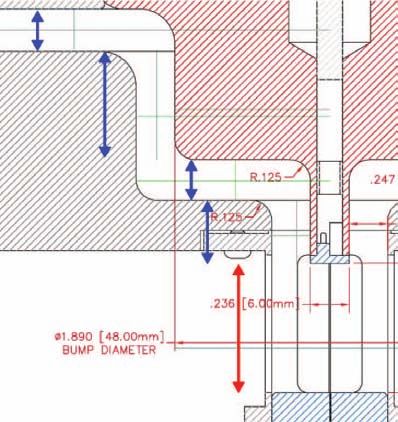
SAND2007-6337
                          Unlimited Release
                         Printed October 2007

      Planar Wire Array Performance Scaling at
      Multi-MA Levels on the Saturn Generator

         B. Jones                                  A.A. Esaulov
      Z Experiments                            Department of Physics

       M.E. Cuneo                                 V.L. Kantsyrev
      Z Experiments                            Department of Physics

      D.J. Ampleford                              A.S. Safronova
      Z Experiments                            Department of Physics

      C.A. Coverdale                         University of Nevada, Reno
 Radiation Effects Research                       Reno, NV 89557

      E.M. Waisman
      Z Experiments                              A.S. Chuvatin
                               Laboratoire de Physique et Technologie des Plasmas
        R.A. Vesey
     ICF Target Design                     Laboratoire du Centre National
                                            de la Recherche Scientifique
         M. Jones                               Ecole Polytechnique
       Z Diagnostics                          91128 Palaiseau, France

Sandia National Laboratories                       L.I. Rudakov
       P.O. Box 5800
  Albuquerque, NM 87185                          Icarus Research
                                                  P.O. Box 30780
                                             Bethesda, MD 20824-0780

                                       3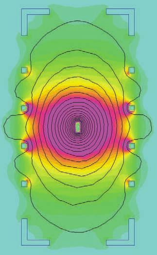
Abstract

A series of twelve shots were performed on the Saturn generator in order to conduct an
initial evaluation of the planar wire array z-pinch concept at multi-MA current levels.
Planar wire arrays, in which all wires lie in a single plane, could offer advantages
over standard cylindrical wire arrays for driving hohlraums for inertial confinement
fusion studies as the surface area of the electrodes in the load region (which serve
as hohlraum walls) may be substantially reduced. In these experiments, mass and
array width scans were performed using tungsten wires. A maximum total radiated
x-ray power of 10±2 TW was observed with 20 mm wide arrays imploding in ∼100
ns at a load current of ∼3 MA, limited by the high inductance. Decreased power
in the 4-6 TW range was observed at the smallest width studied (8 mm). 10 kJ
of Al K-shell x-rays were obtained in one Al planar array fielded. This report will
discuss the zero-dimensional calculations used to design the loads, the results of the
experiments, and potential future research to determine if planar wire arrays will
continue to scale favorably at current levels typical of the Z machine. Implosion
dynamics will be discussed, including x-ray self-emission imaging used to infer the
velocity of the implosion front and the potential role of trailing mass. Resistive
heating has been previously cited as the cause for enhanced yields observed in excess
of jxB-coupled energy. The analysis presented in this report suggests that jxB-
coupled energy may explain as much as the energy in the first x-ray pulse but not
the total yield, which is similar to our present understanding of cylindrical wire array
behavior.

                                           4
Acknowledgment
We thank M. Lopez (1675), G. T. Liefeste (1675), and J. L. Porter (1670) for provid-
ing load hardware and diagnostic support; D.S. Nielsen (1675), L.B. Nielsen-Weber
(1675), R.E. Hawn (1675), and J.D. Serrano (1344) for extensive support of diagnos-
tic installation, fielding, and film processing; L.P. Mix (1652) for IDL data analysis
support; D.A. Graham (1676), S.P. Toledo (1676), R.K. Michaud (1342), and D.M.
Abbate (1342) for load assembly and installation; M.D. Kernaghan (1672), M. Vigil
(1675), and D.H. Romero (1646) for load design and drawing preparation; M.F. John-
son (Team Specialty Products) and J.E. Garrity (1675) for load hardware fabrication
and finishing; T.C. Wagoner (1676), R.L. Mourning (1676), and J.K. Moore (1676)
for B-dot calibration; W.E. Fowler (1671) for voltage monitor support; and K.A.
Mikkelson (1342), B.P. Peyton (1342), T.A. Meluso (1342), B.M. Henderson (1342),
M.A. Torres (1342), J.W. Gergel, Jr. (1342), and the Saturn crew for supporting
accelerator operations. We also thank Center 1300 for providing additional time on
Saturn in order to facilitate completion of the experiments. Work at UNR’s Nevada
Terawatt Facility is supported by DOE/NNSA grant DE-FC52-01NV14050. The re-
search described in this report was funded by Sandia LDRD project #113211, entitled
“Planar Wire Array Performance Scaling at 6 to 10 MA.” We thank Larry Schneider
(1650) and the Science of Extreme Environments LDRD selection team for providing
late-start LDRD funding for this work.
56
Contents

1 Introduction                                                                                             11

2 Planar Wire Array Experiment Design                                                                      15

  Pre-shot 0D-type modeling for load design . . . . . . . . . . . . . . . . . . . . . . . . . . . . 21

  Description of x-ray diagnostics . . . . . . . . . . . . . . . . . . . . . . . . . . . . . . . . . . . . . 27

3 Discussion of Experimental Results                                                                       33

  Tungsten planar wire array total radiated power scaling . . . . . . . . . . . . . . . . . 37

  Planar wire array implosion dynamics . . . . . . . . . . . . . . . . . . . . . . . . . . . . . . . . 42

  Aluminum K-shell radiation from a planar wire array . . . . . . . . . . . . . . . . . . . 48

4 Conclusion                                                                                               51

References                                                                                                 53

                                                     7
List of Figures
2.1 Load hardware drawing, 0◦ view . . . . . . . . . . . . . . . . . . . . . . . . . . . . . . . . 16
2.2 Load hardware drawing, 90◦ view . . . . . . . . . . . . . . . . . . . . . . . . . . . . . . . 17
2.3 Load hardware photos . . . . . . . . . . . . . . . . . . . . . . . . . . . . . . . . . . . . . . . . 19
2.4 Saturn equivalent circuit model . . . . . . . . . . . . . . . . . . . . . . . . . . . . . . . . . 22
2.5 Inner MITL inductance calculation . . . . . . . . . . . . . . . . . . . . . . . . . . . . . . 23
2.6 0D-type calculations of implosion dynamics . . . . . . . . . . . . . . . . . . . . . . . 24
2.7 Electromagnetic calculation of load inductance . . . . . . . . . . . . . . . . . . . . 25
2.8 Diagnostic LOS views . . . . . . . . . . . . . . . . . . . . . . . . . . . . . . . . . . . . . . . . 27
2.9 MLM imager diagnostic . . . . . . . . . . . . . . . . . . . . . . . . . . . . . . . . . . . . . . . 29
3.1 Mass (implosion time) scan x-ray scaling results . . . . . . . . . . . . . . . . . . . 38
3.2 Width scan x-ray scaling results . . . . . . . . . . . . . . . . . . . . . . . . . . . . . . . . 39
3.3 X-ray power scaling with load current . . . . . . . . . . . . . . . . . . . . . . . . . . . 42
3.4 Post-shot 0D modeling of experiments . . . . . . . . . . . . . . . . . . . . . . . . . . . 43
3.5 X-ray imaging of implosion . . . . . . . . . . . . . . . . . . . . . . . . . . . . . . . . . . . . 45
3.6 X-ray imaging after peak x-rays . . . . . . . . . . . . . . . . . . . . . . . . . . . . . . . . 47
3.7 Al K-shell power . . . . . . . . . . . . . . . . . . . . . . . . . . . . . . . . . . . . . . . . . . . . . 49
8List of Tables
2.1 Planar wire array design parameters . . . . . . . . . . . . . . . . . . . . . . . . . . . . . 18
2.2 Predicted planar wire array behavior . . . . . . . . . . . . . . . . . . . . . . . . . . . . 26
3.1 Experimental results: current and timing . . . . . . . . . . . . . . . . . . . . . . . . . 34
3.2 Experimental results: LOS A power/yield . . . . . . . . . . . . . . . . . . . . . . . . 35
3.3 Experimental results: LOS B power/yield . . . . . . . . . . . . . . . . . . . . . . . . 36
3.4 Planar wire array power scaling experiments at 1 MA on Zebra . . . . . . . 41
910
Chapter 1

Introduction

Wire array z pinches are bright, efficient soft x-ray sources, producing up to 250 TW
and 1.8 MJ of radiation [1] in experiments on Sandia’s Z machine [2]. Z-pinch loads
are used for a variety of high energy density physics applications, including inertial
confinement fusion (ICF) studies, K-shell x-ray generation for radiation effects re-
search, and radiation and atomic physics [3]. These loads are typically high wire
number (N∼300) annular arrays with initial diameters in the 20-60 mm range. A
high level of azimuthal symmetry (i.e. high wire number in a cylindrically symmetric
configuration) is believed to be important in producing high x-ray powers as a sym-
metrical implosion produces a more uniform shell with smaller radial width, better
convergence of the mass and current, and a higher level of mass participation in x-ray
production [4, 5].

Recently, planar wire array configurations, in which the wires are arranged as a lin-
ear array confining the mass within a plane, have attracted attention in the z-pinch
community. Experiments on the 1 MA Zebra generator at the University of Nevada,
Reno, produced implosions with < 10 ns x-ray rise times and powers as high as 0.34
TW/cm, comparable to the most powerful cylindrical wire array implosions studied
at that facility [6]. This behavior is surprising, as the standard intuition regarding
cylindrical arrays is that high implosion velocity and a radially narrow plasma shell
are required to achieve a fast rising and high power x-ray pulse. The planar array
distributes the initial mass profile radially, which is not intuitively optimal for provid-
ing high implosion velocity. Laser shadowgraphy indicates, however, that the wires
implode in a cascade, with magnetic Rayleigh-Taylor implosion instabilities being
stabilized to some extent as the implosion front impacts each adjacent wire on its
way toward the axis [7]. This may suggest that a linear array mitigates instabilities
as a multiply nested wire array; nested cylindrical wire arrays have been previously
demonstrated to enhance the radiated x-ray power and shorten the pulse due to mit-
igation of the magnetic Rayleigh-Taylor implosion instability [1] as the current is
switched from the outer to the inner array during the implosion [8].

Previous publications have also discussed the possibility of enhanced Ohmic heating
due to Hall resistivity effects in wire array z pinches, suggesting that the effect might
be exaggerated and thus more clearly observable in planar arrays versus cylindrical
arrays due to a smaller amount of coupled kinetic energy in the planar array case [9, 6].

                                            11
Numerical modeling of wire arrays with a three-dimensional (3D) magnetohydrody-
namic (MHD) code has indicated that resistive heating can play a role in cylindrical
wire array energy deposition, but this contribution is strongest and dominant only af-
ter the main x-ray peak [10]. These simulations assumed Spitzer resistivity, however,
and would not have reflected the effects of enhanced resistivity due to Hall physics if
in fact this phenomenon occurs and is significant in modifying the pinch energetics.
If planar arrays offer an opportunity to assess the role of Ohmic heating in wire array
plasmas, this insight would be generally beneficial to our understanding of z-pinch
physics.
A linear array of wires has also been used to study wire ablation physics, with an
asymmetric single return current post providing a global magnetic field [11]. Plasma
was ablated perpendicular to the plane of the array in a manner consistent with
inductive current division between the wires in this work.
Planar arrays are thus interesting objects from a z-pinch physics perspective, and
their study may shed light on instability mitigation and plasma heating mechanisms.
Beyond basic physics issues, these arrays may be particularly attractive for ICF re-
search due to the reduced volume occupied by the initial load configuration. The
double-ended vacuum hohlraum z-pinch-driven ICF concept [12] which has been ex-
tensively studied on the Z machine [13] relies on a cylindrical primary hohlraum which
also serves as the return current canister for the z-pinch radiation source on axis. The
surface area of the hohlraum is thus constrained by the initial geometry of the cylin-
drical wire array. For a fixed x-ray pulse shape, the peak radiated power required to
produce a given peak hohlraum temperature is given by the relation [14]
³ ´1.1
P ∝ R2 + RL (1.1)
which depends strongly on the hohlraum surface area (R is its radius and L is the
length). The hohlraum temperature requirement is typically fixed by the design of
the fuel capsule which resides in a secondary hohlraum driven from either end by
two z-pinch-driven primary hohlraums. Thus, reducing the hohlraum area (radius
in particular) is attractive for reducing the power requirement placed on the z-pinch
radiation source. The reduction of the wire array area from a cylindrical to a planar
geometry may allow for a significant reduction in primary hohlraum area (the area of
a rectangular current return electrode), as one dimension can be as thin as twice the
anode-cathode feed gap width and no longer has to be wider than the array diameter.
This advantage assumes that planar wire arrays retain their relatively fast rise times
and high powers as they are scaled up to higher drive currents, which is a prime
motivation for the experiments on Saturn discussed in this report. We note that
planar arrays are not required to outperform cylindrical wire arrays–if there is in fact
a reduction in x-ray power, this might be offset by the potential reduction in primary
hohlraum area. Ultimately, x-ray power scaling experiments must be complemented
by integrated hohlraum and capsule modeling in order to determine whether planar-
12array-driven hohlraum energetics competes with the use of compact cylindrical wire
array sources.
Due to the relatively short path lengths through the plasma in the direction normal
to the plane, planar wire arrays may also offer an advantage in mitigating opacity
effects which could limit peak radiated power in high mass, high current, cylindrical
implosions [15].
A final motivating factor is the report from the GIT-12 generator (4.7 MA, 1.7 µs
implosion time) of an increase in Al K-shell yield by a factor of ∼2 compared to
previous cylindrical arrays studied [16]. Wire arrays for producing K-shell x-rays
are typically larger diameter than the compact ICF loads, placing the mass at large
initial diameter so that high implosion velocities and thus plasma temperatures can
be achieved for ionizing to the K shell [17]. It is arguably even less intuitive that
planar wire arrays would benefit K-shell x-ray production, as the mass is radially
distributed rather than initiated at large diameter, but this is another topic that can
be addressed on Saturn.
The following section describes the shot plan and experimental goals for the May-
June 2007 Saturn planar wire array series, including the zero-dimensional (0D)-type
code used to aid in pre-shot load design and post-shot analysis. The x-ray diagnostics
used for these shots are also described. The third chapter presents the experimental
results, including tungsten power scaling experiments for ICF applications, planar
array dynamics and energetics analysis, and Al K-shell x-ray production from a planar
wire array. A concluding chapter summarizes the results and discusses possible future
experiments to assess more fully the power scaling prospects of planar wire arrays.
Primary goals in this report are to provide fairly complete documentation of the
experiments in order to facilitate ongoing collaborations, to outline near-term analysis
goals, and to discuss future directions for study of planar wire arrays.
1314
Chapter 2

Planar Wire Array Experiment
Design

A primary design goal in fielding these experiments at Saturn was to match the im-
plosion time to that expected on the Z machine (100-120 ns) in order to most reliably
consider x-ray power scaling with load current for planar arrays. In addition, an im-
plosion time near 100 ns would be well matched to prior [6] and future experiments
at 1 MA on the Zebra generator, and so these data points could be considered in
a power scaling study. As such, we chose to run Saturn in long-pulse mode, which
has previously been used to study cylindrical arrays with 130-250 ns implosion times
[18, 19]. The Saturn short-pulse mode [5] typically exhibits a peak in the load current
waveform at < 60 ns, which is too short for the desired planar array regime. A new,
larger 12 inch diameter convolute design for Saturn long-pulse mode was fielded as
there is evidence that this convolute has superior powerflow properties and handles
high inductance loads better than the traditional 6 inch convolute [20].

In the early stages of load hardware design, it was decided to be very conservative
with the anode-cathode gap spacing both in the inner MITL feed and in the return
current cage surrounding the wire array load (see Figs. 2.1, 2.2) to reduce risk of load
current arcing. 6-7 mm feed gaps were chosen as the Saturn MITL alignment accuracy
is presently limited. The circuit-coupled 0D-type calculations described below were
performed later in shot planning process (too late to make significant changes to the
load hardware design and still complete the experiments during the FY07 LDRD
cycle). These calculations indicated high load inductances that, when coupled with
the fairly high inner MITL inductances and the 100-120 ns desired implosion time in
the Saturn circuit, led to a roll-over of the load current at levels of ∼3 MA. Only by
taking the implosion time out to 200 ns could this load hardware design approach
the 6 MA current level that was desired in these studies. Thus, the conservative gap
spacing forced an undesirable but unavoidable trade-off between load current and
implosion time. The compromise chosen was to select the wire size and thus load
mass with predicted implosion times near nominally 135 ns, giving load currents of
∼3 MA. This still puts the experiments in the multi-MA range significantly above 1
MA and allows us to start to consider power scaling, but does not achieve the ∼6 MA
levels desirable of more direct relevance to ICF concepts using planar wire arrays on
Z. This planned implosion time is somewhat longer than Zebra at 100 ns, and slightly

                                          15
Cathode
Anode
Debris mitigation
step
“GI”-type
load B-dot
Wire array sensor
Return current cage
Wire
Figure 2.1. Drawing of the load region for the hardware de-
sign used in the May-June 2007 planar array Saturn shot se-
ries, courtesy of M.D. Kernaghan (1672) and M. Vigil (1675).
The view here is parallel to the array of wires. Design re-
quirements included a debris mitigation step feature in or-
der to evaluate an option for multiple shots per day without
MITL cleaning, as well as another debris mitigation bump
(not shown). These features increased the load inductance,
may not actually permit a higher shot rate (see the text for
discussion), and can be eliminated to decrease load induc-
tance.
16Cathode
Anode
Return current
cage
Wire array
Debris
mitigation
step
Figure 2.2. Drawing of the load region for the hardware de-
sign used in the May-June 2007 planar array Saturn shot se-
ries, courtesy of M.D. Kernaghan (1672) and M. Vigil (1675).
The view here is perpendicular to the array of wires. A 20
mm wide wire array is shown, but the same load hardware
was used for all wire array initial widths studied. The gaps
in the load region are very conservative and may possibly be
reduced to 2-4 mm based on other work [21] to decrease the
load inductance.
17Table 2.1. Planar wire array design parameters from the
May-June 2007 Saturn shot series. Table 2.2 lists calculated
implosion times, load currents, and coupled energies, while
Table 3.1 lists experimental results.
Array Array Wire Array Design
Shot Wire height, width, Wire diameter mass implosion
number material h (mm) W (mm) number (µm) (mg/cm) time
3670 W 20 20 40 9.09 0.500 Nominal
3671 W 20 20 40 6.41 0.248 Early
3672 W 20 20 40 12.86 1.000 Late
3673 W 20 20 40 12.86 1.000 Late
3674 W 20 20 40 9.09 0.500 Nominal
3675 W 20 20 40 25.58 3.957 Very late
3682 W 20 20 40 9.09 0.500 Nominal
3683 W 20 8 16 28.21 1.925 Nominal
3684 W 20 12 24 19.25 1.345 Nominal
3685 W 20 12 24 19.25 1.345 Nominal
3686 W 20 8 16 28.21 1.925 Nominal
3688 Al 5056 20 20 40 23.60 0.472 Nominal
longer than the expected nominal short-pulse operating point of the refurbished Z
machine at 120 ns. However, as will be presented below, the implosion times that
were measured experimentally turned out to be closer to 100 ns.
These experiments were designed to determine the scaling of peak x-ray power and
x-ray energy in the main pulse of planar arrays for application to ICF research. The
critical scalings are (1) with implosion time at constant array width (this is a mass
scan), (2) with array width at fixed implosion time, and (3) with peak drive current
at constant implosion time and width. Saturn data are used to evaluate (1) and (2).
Issue (3) is evaluated using data both from Saturn and from the University of Nevada,
Reno, Zebra generator at 1 MA.
Twelve shots were planned and executed on Saturn during May-June 2007. The
load parameters for this series are specified in Table 2.1. As will be discussed in
the experimental results section, shots 3673, 3674, and 3685 were compromised and
will not be used in the scaling studies. The series was designed to accomplish three
basic experiments. First, shots 3670, 3682, 3683, and 3686 comprise a mass (and
implosion time) scan at fixed planar array width. The goal here is to determine
empirically the optimum implosion time for maximizing peak x-ray power with the
chosen load hardware geometry. We also wish to study how the load behaves with
longer implosion times but greater coupled energy (one shot, 3675, was planned with
implosion time near 200 ns and load current in the 5 MA range). Second, shots
183670, 3682, 3683, 3684, and 3686 comprise a width scan where the implosion time
was kept near the nominal 135 ns value but the array size was reduced. The goal
with this set is to determine how compact the array can be made before the x-ray
power drops significantly. In addition, the jxB-coupled energy was expected to vary
over these shots, and we hoped to address the question of whether this can explain
the measured yields, or whether it is necessary to invoke resistive heating. Finally,
one shot, 3688, will provide preliminary information on how effective planar wire
arrays are at producing K-shell x-rays at multi-MA current. For all of these shots,
a series of electrical and x-ray power, yield and imaging diagnostics were fielded as
described below to study the planar array implosion dynamics and attempt to make
some statement about energy coupling.
(a) (b)
(c) (d)
Figure 2.3. Photographs of load hardware from the May-
June 2007 Saturn planar array shots. (a) A 20 mm wide, 20
mm tall, 40-wire W array. (b) A 20 mm wide, 20 mm tall,
40-wire Al 5056 array; the Al 5056 wires hung noticeably
less straight than the W wires. (c) Lower halo assembly and
hanging weights keep the wires under tension. (d) Anode
insert showing the B-dot sensors at 0◦ and 180◦ , and the
return current cage. Courtesy of S.P. Toledo (1676).
Figure 2.3 includes photographs of load hardware for the reader’s reference. The
tungsten wires generally hung quite straight, but the Al 5056 wires in shot 3688 were
somewhat crooked due to the thickness of the wire used. The aluminum wire is more
fragile than the tungsten, and thus it could not be put under greater tension without
an unacceptable amount of wire breakage during assembly. Figure 2.3(c) shows the
weighted wires hanging over a lower halo-type assembly which served to keep the wires
under tension, reduce swinging of weights during transport, and pull the wires into
current contact with the anode. The halo design and wire hanging features are similar
to those used with a single-feed double z-pinch array on Z. During assembly, each wire
was wrapped around one of the four vertical posts shown at the top of Fig. 2.3(a)
with both weighted ends hanging down to become two wires in the planar array. The
small radius of these posts posed problems with wire handling and breakage. It was
also difficult to position the wires in the EDM-cut slots on the cathode when working
near the edges of the wire array due to the proximity of the vertical bars shown at
the top of Fig. 2.3(a). The assembly of these loads was somewhat more difficult than
typical cylindrical wire arrays, and indeed a number of issues were identified that
19should be considered in designing any future planar array load hardware [courtesy of
D. A. Graham (1676)].
The return current canister, important in determining the load inductance, was a
rectangular cage as shown in Fig. 2.3(d). In order to minimize hardware costs for
these shots, the same load hardware was used for all shots with the only difference
being the pattern of EDM-cut wire slots in the anode and cathode. As such, the
return current cage was much larger than necessary for the 12- and 8-mm-width
arrays. Inductance could be reduced in future shots by reducing anode-cathode gaps
in the inner MITL and in the cage, which might serve to increase load current.
For all shots, an inter-wire gap near 0.5 mm was chosen. This decision was made in
order to facilitate assembly of the loads, but also because prior work with cylindrical
wire arrays has indicated that too small an inter-wire gap can be detrimental to x-ray
power performance [19, 22]. The mechanism for degradation has been speculated
to be due to an unfavorable modification of the ablated plasma pre-fill profile as
wire number is changed [23] or a merging of the current-carrying coronal plasma
surrounding the wires early in time, allowing current to jump between adjacent wires
and compromising the uniformity of the current path [24]. It is not clear that either
of these mechanisms would be relevant to planar wire arrays, which already have
a significant initial mass distribution interior to the load, and in which the current
distribution between the wires is likely inductive with stronger current density on the
outer edges of the array. Also, unpublished experiments with planar arrays at 1 MA
at the University of Nevada, Reno, showed that power decreased for inter-wire gaps
of both 0.2 mm and 1 mm compared to 0.5 mm [25].
Given these physics concerns and the practical concerns associated with building the
loads, we fixed the inter-wire gap near 0.5 mm which placed a constraint on the
parameter space of the load design. This choice, coupled with the choice of array
widths and implosion times in Table 2.1, resulted in some loads having relatively
large wire sizes approaching 30 µm diameter. This in itself poses a concern regarding
wire initiation and ablation behavior, and clearly future experiments with higher wire
number and smaller inter-wire gaps could be interesting. Planar arrays tend to have
large mass relative to cylindrical arrays of the same spatial scale and implosion time
due to the initial distribution of this mass near the array axis, which is what leads
to the increased wire size requirement. We note also that for high-current planar
array experiments it might be possible to consider using a foil ribbon in place of a
planar wire array, which would certainly change the ablation and perhaps implosion
dynamics.
20Pre-shot 0D-type modeling for load design
The load widths and implosion times were chosen to meet experimental goals as dis-
cussed above. With the inter-wire gap also fixed, the remaining as-yet-unspecified
design parameter is the wire size. This must be chosen to give the array the appro-
priate mass so that the appropriate implosion time will be achieved when coupled to
the generator. In the case of cylindrical wire arrays, 0D thin-shell calculations are
typically employed in load design calculations to choose the load mass [26]. Here, the
wire array is approximated as a zero-thickness shell of mass, and the radial equation
of motion is solved numerically in the azimuthally symmetric case while also coupling
the evolution of the load inductance to the generator circuit. This calculation is less
straightforward for a planar array, which lacks cylindrical symmetry and for which
load inductance is a more complicated function of geometry than the cylindrical case,
where L ∼ 2h log(R/r) for a wire array of height h, radius r and return current
canister radius R. A technique for performing a 0D-type simulation for an arbitrary
arrangement of wires and return current structures has been developed, however, and
was employed in collaboration with A. A. Esaulov (University of Nevada, Reno) in
designing the planar array loads for the May-June 2007 Saturn shots. Termed the
“wire dynamics model” [27], the technique can be applied to single or multiply nested
cylindrical arrays, or planar wire arrays. The model implicitly includes inductive di-
vision of current between the wires at each time step, and essentially applies F=ma
to each wire in order to track its trajectory. Inductive current division still allows
current to be distributed throughout the wires in a planar array, but causes current
to peak in the few wires near the edge of the array with the outermost wires carrying
a factor of 2-3 times more current than the innermost wires [27]. We expect this
to be the most reasonable assumption for planar arrays, given the observations that
the inner wires ablate and so must carry some current [6], but also that the inner
wires experience little acceleration while the implosion commences at the outer wires
and cascades inward [7] implying that somewhat less current flows in the inner wires.
Modeling with inductive division best reproduces the latter observation. We note,
however, that modeling of the planned Saturn planar loads was also carried out by
A. S. Chuvatin (Ecole Polytechnique) with the assumption of uniform (i.e. resistive)
current division between the wires, and similar implosion times, peak currents, and
coupled energies were obtained.
The 0D planar array simulations included coupling to the Saturn circuit model shown
in Fig. 2.4. The voltage at the post-hole convolute was estimated using the expression
q
+Z 2 2
f Iu − Id , Rising current: Id < Iu
VP H = q (2.1)
−Z I 2 − I 2 , After peak: I > I
f d u d u
The inner MITL inductance was calculated as described in Fig. 2.5. The load induc-
tance was calculated internally in the 0D code, including inductive division between
21Ru Lu VPH
Zf Ll
~V C
Iu Id
Figure 2.4. The Saturn generator was modeled with the
equivalent circuit shown in performing 0D-type implosion cal-
culations. Ru =0.15 Ω is expected for Saturn with 36 modules,
but Ru =0.2 Ω was used here as the May-June 2007 shots were
conducted with only 30 modules. Zf =0.25 Ω was assumed,
Eq. 2.1 was used for VP H , and Lu =5 nH. Courtesy of A. A.
Esaulov (University of Nevada, Reno).
wires and appropriate boundary conditions on the return current cage to determine
its current distribution. The return current cage was modeled as a series of station-
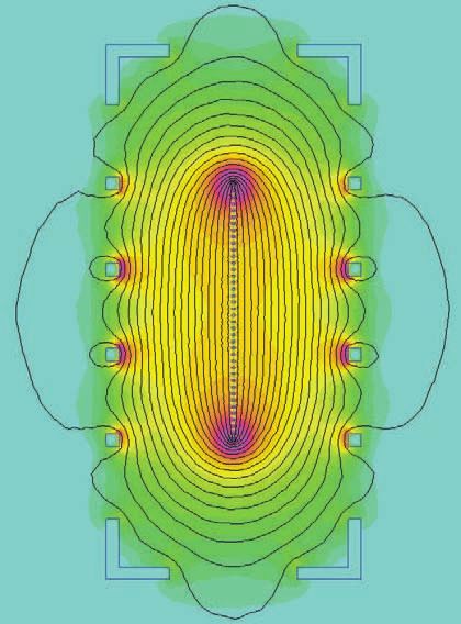
ary filaments, as shown in Fig. 2.6(a). Figure 2.6(c-e) shows magnetic field lines
within the load region for the initial configurations of planar arrays of 8, 12, and 20
mm width as calculated by the code. The initial calculated load inductances are indi-
cated, and are seen to be quite high due to the geometry of the magnetic field and the
size of the return current structure. These initial load inductances were also verified
by electromagnetic calculations with a more accurate return current cage geometry
(Fig. 2.7). In the case of the smaller width loads in Fig. 2.6, it is clear that the
return current cage is excessively large, leading to a large volume filled with magnetic
energy and correspondingly a large inductance. Again, this was because the same
load hardware was used for all shots in order to reduce costs. Future experiments
with a more closely coupled return current can could be designed in order to reduce
the inductance and increase the load current. Figures 2.6(c-e) also give some intuition
as to why the implosion starts in the outer wires and cascades through the stationary
inner wires–tension in the magnetic field lines is greatest at the edges of the array
where curl of B (and hence j and then also jxB) is large. Figure 2.7(a) indicates that
the magnetic pressure is greatest at the edges of the array as well.
Figure 2.6(b) shows an example of implosion calculations for wire arrays of various
widths, designed so that they have the same implosion time. Here x indicates the
22h=0.627cm, R=15.2cm, r=2.4cm
L~2h ln(R/r)~2.32 nH
h=1.7cm, R=3cm, r=2.4cm
L~2h ln(R/r)~0.76 nH
h=0.627cm, w=2.8cm, R=3cm
L~2h ln(4R/w)~1.83 nH
h=1cm, w=2.8cm, d=0.6cm
L~4πhd/(2w)~1.35 nH
More exact L~0.91 nH
Load inductance calculated
in 0D implosion code
Figure 2.5. The inner MITL inductance for the load hard-
ware used in May-June 2007 Saturn planar array shots was
calculated as shown. The inductance of a cylindrically sym-
metric MITL section is estimated with the standard formula
L ∼ 2h log (R/r), where h is the height, R is the outer radius,
and r is the inner radius. The inductance of each strip line
section is estimated as L ∼ 4πhd/ (2w), where h is the height,
w the width, and d is the anode-cathode gap spacing, and the
expression is valid for d¿w; the factor of 2 accounts for the
two current returns. A more exact analytic treatment was
also applied to the strip line sections [28]. A net inner MITL
inductance of 5 nH was then used for all of these shots in
0D-type implosion calculations. Courtesy of A. S. Chuvatin
(Ecole Polytechnique).
23(a) -2 -1 0 1 2 1.5
1.5 1.5 1 (c)
1 1 0.5
y (cm)
0
0.5 0.5
y (cm)
-0.5
0 0
-1
-0.5 -0.5 W= 20 mm ; N = 40 ; Lload = 4.46 nH
-1.5
-1 -1 1.5
-1.5 -1.5 1 (d)
-2 -1 0 1 2 0.5
y (cm)
x (cm) 0
(b)
x (cm) I (MA) -0.5
1 3 -1
W = 20 mm W= 12 mm ; N = 24 ; Lload = 6.28 nH
-1.5
0.8 W = 12 mm
1.5
W = 8 mm
0.6
2
1 (e)
0.5
y (cm)
0.4 0
1
-0.5
0.2
-1
W= 8 mm ; N = 16 ; Lload = 7.91 nH
0 0 -1.5
0 40 80 120 160 200 -2.5 -2 -1.5 -1 -0.5 0 0.5 1 1.5 2 2.5
t (ns) x (cm)
Figure 2.6. Planar array load design was aided by 0D-type
calculations of trajectory and current. (a) The return current
cage was modeled as a set of current filaments (black circles).
(b) Load mass was chosen here for constant implosion time
at several array widths W and wire numbers N. (c-d) Mag-
netic field lines for initial load configurations at various W, N;
initial inductance Lload is calculated assuming inductive cur-
rent division between the wires. Courtesy of A. A. Esaulov
(University of Nevada, Reno).
24(a) (b)
Figure 2.7. (a) An electromagnetic code calculation of ini-
tial load inductance with accurate return current cage geom-
etry gives 4.26 nH for an array of 20 mm width, in close
agreement with the simplified cage model of Fig. 2.6(c). (b)
The inductance rises to 10.63 nH for a z-pinch current chan-
nel compressed to 2 mm × 1 mm, a convergence ratio of 10.
The magnetic field lines are shown along with color contours
indicating field strength. This figure also indicates that the
load inductance will be most sensitive to the feed gap spacing
in the direction perpendicular to the wire array; the config-
uration of the cage bars may also be important. Courtesy of
A. S. Chuvatin (Ecole Polytechnique).
25Table 2.2. Predicted planar wire array load behavior, cal-
culated with a 0D-type code including a Saturn circuit model
in advance of the experiments and used to guide the choice of
load parameters in Table 2.1. Table 3.1 lists experimental re-
sults for comparison. Courtesy of A. A. Esaulov (University
of Nevada, Reno).
Design Coupled
Shot implosion Implosion Peak load energy (kJ)
number time time (ns) current (MA) (xf = 100µm)
3670 Nominal 138 2.5 41
3671 Early 124 2.0 25
3672 Late 152 3.0 64
3673 Late 152 3.0 64
3674 Nominal 138 2.5 41
3675 Very late 200 4.7 140
3682 Nominal 138 2.5 41
3683 Nominal 125 2.3 34
3684 Nominal 135 2.5 44
3685 Nominal 135 2.5 44
3686 Nominal 125 2.3 34
3688 Nominal 137 2.5 39
position of the outermost wire which becomes the implosion front as it sweeps up
the mass held in the interior wires. This code does not include wire ablation, which
could impact the implosion trajectory by influencing when the outer wire begins to
move. Given the large amount of mass already interior to the implosion front in a
planar array, we might expect ablation to play less of a role in the dynamics and
energy coupling than in a compact cylindrical wire array; this is a topic of continuing
research, however. Figure 2.6(b) also shows the calculated load current resulting from
coupling the wire array trajectory calculations with the Saturn circuit model in Fig.
2.4. It is seen that the large load inductance and short implosion times (for Saturn
long-pulse mode) limit the current to near 3 MA.
In choosing the wire sizes and masses in Table 2.1, the 0D-type code was used itera-
tively for each shot to arrive at a wire size that met the implosion time requirement
given the specified array width and wire number. Another constraint was available
wire sizes in the Center 1600 inventory, which for a few shots limited the choice of
array mass so that an exact match in predicted implosion time was not possible for
all shots in the width scan experiment. The results of the pre-shot modeling is shown
in Table 2.2. As will be seen in the section of this report discussing the experimen-
tal results, these predictive simulations did a reasonable job of accurately predicting
the load current via the Saturn circuit coupling. Although the pre-shot predicted
26implosion times were somewhat late, the general trends were captured. Post-shot
comparison between the experimental results and the model can be used to refine the
circuit parameters for better fidelity in future shot planning.
Table 2.2 also indicates the jxB-coupled energy for each shot simulation. This is
essentially the kinetic energy of the imploding mass, as is the case in a 0D simulation
of a cylindrical array, but it also includes energy that is dissipated as the wires collide
sequentially during the implosion. Momentum is conserved during each collision, but
energy is not and the lost kinetic energy is tracked by the code in order to quote the
total coupled energy via jxB work at the end of the simulation. As with 0D models of
cylindrical arrays, an effective final position for the implosion front must be specified
at which the simulation will end and the jxB work will cease. In these simulations,
that final value was taken as xf = 100 µm, which is likely too small. Based on x-ray
imaging that will be presented, a value of xf = 500 µm may be more reasonable, and
these calculations should be repeated to study the sensitivity of the coupled energy to
xf . For now, we can consider this to be a reasonable estimate of the coupled energy
which may in fact be an upper limit. The issue of energy coupling will be discussed
further in the context of post-shot simulations of experimental data presented below.
Description of x-ray diagnostics
Three lines-of-sight (LOS) were employed in the May-June 2007 Saturn planar array
shot series, each at 35◦ from the horizontal. Views from each LOS are shown in Fig.
2.8, with the position of the pinch shown by a thin gray column on the hardware axis.
These views were used to quantify and correct for the limitation in axial field of view
of the stagnated plasma in analyzing the diagnostic data.
LOS A and LOS B each fielded a 5 µm kimfol filtered x-ray detector (XRD) [29]
(a) (b) (c)
Figure 2.8. Orthographic views of the load region at 35◦
below the horizontal from (a) LOS A, (b) LOS B, and (c) LOS
C. The z-pinch axis is indicated by a thin gray column. The
rulers shown are in the plane perpendicular to the viewing
line of sight. Courtesy of M. Vigil (1675).
27and a bare Ni bolometer [30] to characterize the total radiated soft x-ray power and
yield. The bolometer provides a measurement of total yield expected to be accurate
to 15%. We follow the typical practice of normalizing the XRD waveform to the
total bolometer yield in order to infer the x-ray power pulse, which is expected to be
accurate to 25%. This power waveform is then integrated to infer the x-ray yield in the
pre-pulse (defined as the time prior to the extrapolation of the 20-80% rise to zero), the
rise up to the main x-ray peak, and the energy in the first pulse prior to the back side
of the full width at half maximum (FWHM). This procedure assumes that the XRD
waveform, which responds to photons in the window below the carbon edge at 284
eV, is representative of the total x-ray radiation pulse. The correspondence between
the XRD and the smoothed, differentiated bolometer signal was verified on shot 3675
where the pulse was broad and fairly smooth, and such a bolometer differentiation
could be reasonably carried out. There is a concern for Al loads that the K-shell
photons can pass through the 5 µm kimfol filter above 1 keV and dominate the XRD
signal over the photons passing through the lower transmission carbon window [31],
however this is more of a concern for shots such as on Z where a very significant
fraction of the total radiated power (∼30%) is emitted in the Al K-shell range. A
Lambertian correction for an optically thick surface radiator was performed on the
bolometer yield (and thus x-ray power) data quoted, but at the 35◦ viewing angle this
amounted to only a -5% adjustment from the calculated 4π (optically thin emission)
values.
Photoconducting detectors (PCDs) [32, 33, 34] filtered with 8 µm Be + 1 µm CH were
also fielded on LOS A and B to look at radiated power at photon energies > 1 keV.
In the case of the Al z-pinch studied (shot 3688), these can be used quantitatively
to determine the K-shell power and yield. For this analysis, it is assumed that all of
the K-shell energies is emitted at the Al Ly-α photon energy (1.7 keV) for purposes
of performing a filter transmission correction. This is the brightest line observed
spectroscopically, and the filter transmissions are high enough at the K-shell energies
(≥80 %) that the resulting error due to uncertainty in the spectral shape is less than
10%. Power and yield values quoted represent the average of 4π and Lambertian-
corrected values due to uncertainty in the opacity of the K-shell emission, but as noted
above this is a small adjustment. We expect Al K-shell power and yield values quoted
to be accurate to 25%. For tungsten pinches, whose PCD signals are smaller than for
Al K-shell, the detectors are likely responding to the tail of a broad continuum, and
so quantitative analysis of PCD data is not practical without detailed and accurate
spectral shape characterization data which are not available. It is still useful in some
cases, however, to qualitatively observe when the > 1 keV photon emission is turning
on for W loads.
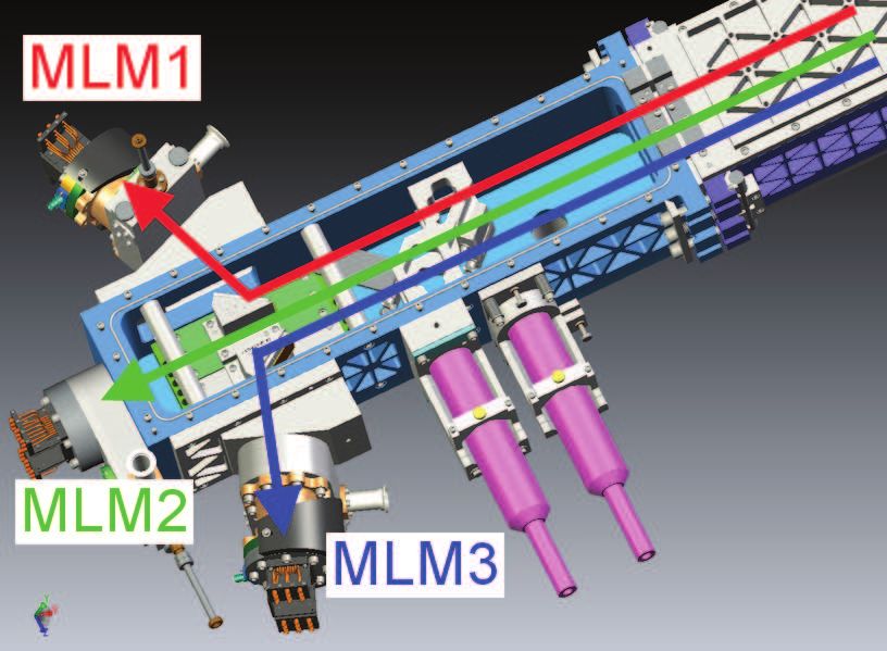
A pinhole camera diagnostic was also fielded on LOS B to perform 1 ns gated x-ray
imaging of the planar array implosions in order to study their dynamics. As shown
in Fig. 2.9, this instrument includes three 8-frame microchannel plate cameras. Two
cameras (MLM1 and MLM3) view the z pinch via reflection from multilayer mirrors,
which act as monochromators and reflect narrowband photons in the 100-700 eV x-
28Reflectivity (%)
Z-pinch Pinhole 25
source (c)
(a)
MLM
0
Planar 25
MLM (d)
Trans. (%)
277 eV
Filter
Filter
(b) 0
Time-resolved 260 270 280 290
imaging detector Photon energy (eV)
(e)
Figure 2.9. A time-resolved pinhole camera diagnostic is
employed on Saturn which includes both standard filtered
pinhole cameras (a) and pinhole cameras that reflect from a
multilayer mirror monochromator (b). The multilayers re-
flect a narrow band of photons near 277 eV (c) while an alu-
minized kapton filter attenuates visible light and second order
reflection (d). The Saturn instrument (e) combines two eight-
frame 277 eV photon energy MLM cameras (MLM1, MLM3)
with an eight-frame standard pinhole camera (MLM2) fil-
tered for >1 keV photons. Figures (a-d) are reprinted with
permission from B. Jones et al., “Monochromatic X-Ray Self-
Emission Imaging of Imploding Wire Array Z-Pinches on the
Z Accelerator,” IEEE T. Plasma Sci. 34, 213 (2006), Figs.
c
1, 2. °2006, IEEE.
29ray range. For these experiments, two Cr/C mirrors were fielded to reflect 277 eV
photons with < 10 eV bandpass as shown in Fig. 2.9(b). The third camera (labeled
MLM2 but not incorporating a mirror) is a standard filtered pinhole geometry, and
8 µm Be + 1 µm CH was employed to match the PCDs and image > 1 keV photons.
May-June 2007 is the first shot series for which this instrument has been fielded on
Saturn, where it will remain available to support future shots on the facility. A similar
version of this diagnostic has been previously fielded on the Z machine [35, 36, 37, 38]
and will be available as a core diagnostic on the refurbished Z machine.
A time-integrated crystal spectrometer (TIXTL) [39, 32] was fielded on LOS C for
one shot only (3688) to measure the Al and Mg K-shell lines. This instrument used
a convex KAP crystal with 2 inch bending radius and 20◦ crystal rotation with a 0.5
mil Be filter and a 300 µm slit for one-dimensional (axial) spatial resolution of ∼900
µm at 1/2 magnification. Al 5056 wires were used for this shot, which have a 5% Mg
dopant content so that Mg K-shell lines are less likely to be affected by opacity than
Al lines (although it is still a consideration given the relatively high mass fielded).
Electrical diagnostics on these Saturn shots included MITL B-dots and GI-type load
B-dots for measuring MITL and load current. Two shots (3674 and 3685) fielded a
voltage monitor probe that inductively coupled the cathode above the load to the
MITL wall across the convolute in order to measure the voltage and inductance of
the load [40]. The installation of this monitor had to be performed after the wire
array load was installed as it was designed to attach to the retaining nut above
the load cathode. This led to a disturbance of the load and MITL regions as the
diagnostician was required to stand on the MITLs and mount to the hardware feature
that was holding the wire array in place. As a result, it was noticed post-shot on
3674 that wires had been broken during this pre-shot alignment (untarnished weights
were found lying on the bottom lid after breaking vacuum), and so data from that
shot is unusable. This problem did not reoccur on shot 3685, but on both shots the
MITL current was higher than usual and the load current and x-ray output were low.
We believe that the MITL was misaligned while it was being walked on, causing a
post-hole convolute short. Thus, the data from 3685 cannot be used as part of a
width scaling scan, however the load current and x-ray measurements are valid and
this shot stands on its own for investigation of planar array dynamics and current
scaling. This is important because it is the only tungsten wire array fielded for which
the MLM imager was timed early enough to observe the implosion of the planar wire
array during the rise of the main x-ray pulse. Images of the implosion were also
obtained on 3688, the Al 5056 planar array.
Two diagnostic timing problems were discovered during this shot series. One was a
∼30 ns error in the MLM imager frame timing due to an error in the header file. This
resulted in images being recorded later than we had thought, thus most of the images
obtained were after peak x-ray power. A ∼5 ns timing shift was found for the LOS
A and LOS B bolometers by comparing to a machine B-dot reference signal in that
screen box. M. A. Torres (1342) noted the error and corrected the header to account
30for it, and is continuing to track down the source of the discrepancy. Both of these
errors will be eliminated in future shots, and can be corrected for post-shot for the
May-June 2007 Saturn shots. Timing is expected to be accurate to 1 ns on Saturn.
3132
Chapter 3

Discussion of Experimental Results

As discussed above, shots 3670, 3671, 3672, 3675, and 3682 constitute a mass and
implosion time scan, while shots 3670, 3682, 3683, 3684, and 3686 comprise a width
scan for planar arrays from the May-June 2007 Saturn shot series. Shot 3674 suffered
from a post-hole convolute short as well as broken wires and so is unusable. Shot
3685 also appeared to suffer a post-hole convolute short and lower load current and so
cannot be included in the width scan, however we will include this shot in a current
scaling comparison and will use imaging data to address planar array dynamics. For
shot 3673, we attempted to shoot a second shot in a single day by leaving the MITLs
in place and not refurbishing them. This shot produced comparable current and
yield to shot 3672, which was otherwise identical, however the x-ray pulse shape was
changed and the power reduced. We have elected not to include this shot in the
scaling studies as there is residual concern regarding whether the dirty MITLs could
have somehow impacted the wire array performance.

Table 3.1 shows measured load current, implosion time, x-ray rise time and FWHM
(for both LOS A and B XRD measurements) for all of the planar array shots. Tables
3.2 and 3.3 indicate the measured x-ray yields in the prepulse, rise to peak, main pulse,
and total pulse for LOS A and B respectively. These tables also indicate the calculated
coupled energy estimated with the 0D-type code described above which was in this
case run post-shot using measured load current waveforms rather than including the
Saturn circuit model. We consider this to be our most reliable estimate of jxB
input energy for each shot, although note the concern mentioned above regarding
the choice of final stagnation position in the model. In the following sections we will
plot and make reference to these data, but they are included in tabular form here for
completeness in this report.

We note that the implosion times listed in Tables 3.2 and 3.3 are somewhat shorter
than the pre-shot predictions in Table 2.2. This is fortunate in some sense, as the
measured current levels were in the ∼3 MA range as predicted, but the nominal
implosion time is near 100 ns, in the correct range for comparison with Zebra and Z
generators. The discrepancy is something to be considered, though, and we discuss
this further in the section on planar array dynamics.

                                           33
Table 3.1. Experimental data for the Saturn shots
described in Table 2.1, including load current from B-dot
diagnostics and x-ray pulse timing from XRDs on LOS A
and B. Implosion time is defined as the time of peak total
x-ray power relative to the extrapolation to zero of the linear
rise of the load current (45-70% of peak current or 4 MA for
shot 3675).
m Shots used in mass (implosion time) scan.
w Shots used in width scan.
i Shots used for current scan with Zebra data in Table 3.4.
∗ Voltage monitor was fielded, but reduced load current
perhaps due to post-hole convolute short was observed.
† Wires broken pre-shot; data are not usable.
‡ MITLs not pulled and cleaned prior to shot; data may or
may not be usable.
LOS A LOS B
Peak 10-90% 10-90%
Shot current Implosion rise time FWHM Implosion rise time FWHM
number (MA) time (ns) (ns) (ns) time (ns) (ns) (ns)
3670mw 2.8 96.0 16.6 16.7 96.0 19.3 15.4
3671m 2.4 81.4 20.6 25.7 92.2 28.4 12.3
3672m 3.6 101.1 9.2 8.0 100.9 8.4 6.4
3673‡ 3.4 110.6 22.6 25.4 110.4 24.6 25.2
3674∗† 2.1 109.7 20.0 19.5 104.7 34.2 25.9
3675m 6.0 175.5 35.1 24.2 175.5 26.2 31.0
3682mw 3.0 91.2 11.3 16.1 91.0 12.5 17.1
3683wi 3.2 99.4 18.2 13.5 94.4 14.8 17.5
3684wi 3.0 94.8 13.8 13.8 93.4 13.2 13.0
3685∗i 2.6 103.5 19.4 19.6 103.3 18.8 19.7
3686wi 2.6 90.9 12.7 13.8 90.7 14.8 15.1
3688 3.6 90.4 15.3 19.5 90.0 12.9 19.3
34Table 3.2. Experimental total radiated x-ray power and
yield data from diagnostics on LOS A for the Saturn shots
described in Table 2.1. Calculated coupled energy is from
0D-type modeling using the measured current waveform and
assuming xf = 100µm (courtesy of A. A. Esaulov, University
of Nevada, Reno).
m Shots used in mass (implosion time) scan.
w Shots used in width scan.
i Shots used for current scan with Zebra data in Table 3.4.
∗ Voltage monitor was fielded, but reduced load current
perhaps due to post-hole convolute short was observed.
† Wires broken pre-shot; data are not usable.
‡ MITLs not pulled and cleaned prior to shot; data may or
may not be usable.
Yield Peak Yield to Calculated
Peak Yield in to peak power back of Total coupled
Shot power prepulse power ×FWHM FWHM yield energy
number (TW) (kJ) (kJ) (kJ) (kJ) (kJ) (kJ)
3670mw 11.9 14.1 99.3 197.6 197.9 282.2 66
3671m 6.3 6.6 69.3 162.6 143.1 175.8 46
3672m 12.2 15.9 59.5 97.9 113.8 281.6 113
3673‡ 7.8 14.2 122.6 199.1 203.6 273.0 113
3674∗† 3.6 7.7 52.9 69.4 73.2 92.4 NA
3675m 7.6 21.3 118.3 183.6 198.3 304.5 288
3682mw 8.7 10.4 52.5 140.3 126.0 177.0 74
3683wi 4.6 9.2 43.1 62.1 63.4 152.3 63
3684wi 7.1 11.0 58.7 97.8 101.0 167.1 64
3685∗i 3.9 6.7 36.3 75.9 77.9 106.0 47
3686wi 5.8 6.7 44.1 80.6 74.3 186.7 46
3688 5.5 7.8 47.4 106.8 104.6 215.0 109
35Table 3.3. Experimental total radiated x-ray power and
yield data from diagnostics on LOS B for the Saturn shots
described in Table 2.1. Calculated coupled energy is from
0D-type modeling using the measured current waveform and
assuming xf = 100µm (courtesy of A. A. Esaulov, University
of Nevada, Reno).
m Shots used in mass (implosion time) scan.
w Shots used in width scan.
i Shots used for current scan with Zebra data in Table 3.4.
∗ Voltage monitor was fielded, but reduced load current
perhaps due to post-hole convolute short was observed.
† Wires broken pre-shot; data are not usable.
‡ MITLs not pulled and cleaned prior to shot; data may or
may not be usable.
Yield Peak Yield to Calculated
Peak Yield in to peak power back of Total coupled
Shot power prepulse power ×FWHM FWHM yield energy
number (TW) (kJ) (kJ) (kJ) (kJ) (kJ) (kJ)
3670mw 11.7 25.7 77.8 180.6 160.4 306.7 66
3671m 9.2 3.0 120.3 113.2 139.0 195.8 46
3672m 11.3 17.7 56.3 72.3 89.0 315.3 113
3673‡ 7.7 16.0 116.0 195.1 191.9 305.0 113
3674∗† 2.9 8.7 32.9 76.1 68.3 113.1 NA
3675m 8.4 28.0 123.7 259.7 242.8 426.9 288
3682mw 8.4 13.9 51.9 144.2 133.6 218.1 74
3683wi 4.3 9.7 31.3 75.6 74.0 201.3 63
3684wi 8.1 11.4 61.1 105.6 112.0 224.3 64
3685∗i 3.9 7.5 36.7 77.4 77.1 133.6 47
3686wi 5.0 9.0 42.9 75.0 70.3 232.1 46
3688 4.7 7.0 38.3 89.9 83.0 267.5 109
36Tungsten planar wire array total radiated power
scaling
Figure 3.1 shows total radiated power, 10-90% rise time, FWHM, and yield over
various ranges of the x-ray pulse for the mass scan data set. From Fig. 3.1(a-b),
the optimal mass for x-ray power generation using this load hardware style appears
to be ∼1 mg/cm, although the limited number of data points and the shot-to-shot
variation observed in the twice-repeated experiment at 0.5 mg/cm make it difficult to
be precise. The highest power shot was at 12 TW, though to be conservative given the
apparent shot-to-shot variation we quote 10±2 TW as the optimal power obtained
with these 3 MA planar wire arrays at 20 mm width and 100 ns implosion time. It is
clear that for the shortest implosion time studied (∼85 ns, 0.248 mg/cm, shot 3671)
the yield was reduced and the rise-time increased. For the longest implosion time and
highest mass case (175 ns, 3.957 mg/cm, shot 3675) the yield has actually increased
beyond any of the shorter implosion time shots, although the rise-time and FWHM
have also increased, resulting in a drop in the peak x-ray power.
From Fig. 3.1(c), we see that the 0D-calculated coupled energy increases with mass
and implosion time, which makes sense as the peak load current is also increasing.
We can make the nominal statement that the calculated jxB-coupled energy explains
the yield in the first x-ray pulse. It is clear that our optimistic estimation of jxB in-
put energy does not explain the total x-ray yield. This is not particularly surprising;
the same observation has been previously made for cylindrical wire array implosions
[41, 42], with proposed explanations including additional plasma compression and
PdV work post-stagnation [43], m=0 [44, 45, 46] or m=1 [10] instabilities enhancing
resistive or inductive energy deposition, and Hall effect enhancements in Ohmic heat-
ing [9]. It is interesting that the calculated coupled energy comes close to explaining
the total yield for the highest mass case, while it does not even explain the yield
to peak x-rays for the lightest load. This could indicate that resistive heating (or
whatever energy coupling mechanism is at work) can play a more or less significant
role in the overall energy balance depending on the location in parameter space of a
particular load design. The data do not exclude the possibility that a possible Ohmic
mechanism deposits a fixed amount of energy in the z pinch for all masses studied in
addition to the kinetic energy coupled (which increases with mass). Finally, we note
that there appears to be a systematic trend in comparing data from LOS A and B
(on which independent bolometers and XRDs were fielded): they agree well in the in
first x-ray power pulse, but LOS B repeatedly shows a higher total x-ray yield due
to an enhanced tail of the x-ray pulse. This could indicate that opacity is playing a
role in limiting the late-time power from LOS A, which views the pinch at an angle
to the array plane normal direction. We do not have imaging on LOS A, though, so
we can’t exclude the possibility of one of the return current cage bars occluding some
of the omission from the broader plasma column that is seen after the x-ray peak (to
be discussed in the following section on implosion dynamics).
37You can also read