Smoke-charged vortices in the stratosphere generated by wildfires and their behaviour in both hemispheres: comparing Australia 2020 to Canada 2017
←
→
Page content transcription
If your browser does not render page correctly, please read the page content below
Atmos. Chem. Phys., 21, 7113–7134, 2021
https://doi.org/10.5194/acp-21-7113-2021
© Author(s) 2021. This work is distributed under
the Creative Commons Attribution 4.0 License.

Smoke-charged vortices in the stratosphere generated by
wildfires and their behaviour in both hemispheres:
comparing Australia 2020 to Canada 2017
Hugo Lestrelin, Bernard Legras, Aurélien Podglajen, and Mikail Salihoglu
Laboratoire de Météorologie Dynamique, UMR CNRS 8539, IPSL, PSL-ENS/École Polytechnique/Sorbonne Université,
Paris, France

Correspondence: Bernard Legras (legras@lmd.ens.fr)

Received: 21 November 2020 – Discussion started: 30 November 2020
Revised: 26 March 2021 – Accepted: 29 March 2021 – Published: 10 May 2021

Abstract. The two most intense wildfires of the last decade       1   Introduction
that took place in Canada in 2017 and Australia in 2019–
2020 were followed by large injections of smoke into the          A spectacular consequence of large summer wildfires in
stratosphere due to pyro-convection. After the Australian         mid-latitude forests is the generation of pyro-cumulonimbus
event, Khaykin et al. (2020) and Kablick et al. (2020) dis-       (PyroCb) that can reach the lower stratosphere during ex-
covered that part of this smoke self-organized as anticyclonic    treme events (Fromm et al., 2010). The combustion products
confined vortices that rose in the mid-latitude stratosphere      and accompanying tropospheric compounds (e.g. organic
up to 35 km. Based on Cloud-Aerosol Lidar with Orthogonal         and black carbon, smoke aerosols, condensed water, carbon
Polarization (CALIOP) observations and the ERA5 reanal-           monoxide, and low ozone) that are lifted to the stratosphere
ysis, this new study analyses the Canadian case and finds,        can survive several months and be transported over consid-
similarly, that a large plume had penetrated the stratosphere     erable distances (Fromm et al., 2010; Yu et al., 2019; Kloss
by 12–13 August 2017 and then became trapped within a             et al., 2019; Bourassa et al., 2019), filling the mid-latitude
mesoscale anticyclonic structure that travelled across the At-    band and sometimes reaching the tropics (Kloss et al., 2019).
lantic. It then broke into three offspring that could be fol-     As black carbon is highly absorptive of the incoming solar
lowed until mid-October, performing three round-the-world         radiation, the resulting heating produces buoyancy (de Laat
journeys and rising up to 23 km. We analyse the dynami-           et al., 2012; Ditas et al., 2018) and an additional lift of the
cal structure of the vortices produced by these two wildfires     undiluted parts of the plume by several kilometres in the
and demonstrate how the assimilation of the real tempera-         stratosphere (Khaykin et al., 2018; Yu et al., 2019). This ef-
ture and ozone data from instruments measuring the signa-         fect enhances the dispersion and, by increasing the altitude,
ture of the vortices explains the appearance and maintenance      ensures a longer lifetime in the stratosphere (Yu et al., 2019),
of the vortices in the constructed dynamical fields. We pro-      enhancing the amplitude of the radiative effect on climate
pose that these vortices can be seen as bubbles of small, al-     that has been estimated to be comparable to moderate vol-
most vanishing, potential vorticity and smoke carried verti-      canic eruptions (Peterson et al., 2018; Khaykin et al., 2020).
cally across the stratification from the troposphere inside the      The magnitude of Australian wildfires of the 2019–
middle stratosphere by their internal heating, against the de-    2020 summer season exceeded all previously known events
scending flux of the Brewer–Dobson circulation.                   (Khaykin et al., 2020). A striking discovery was the obser-
                                                                  vation that a part of the stratospheric smoke plumes self-
                                                                  organized as anticyclonic vortices that persisted for between
                                                                  1 and 3 months (Kablick et al., 2020; Khaykin et al., 2020;
                                                                  Allen et al., 2020); the most intense smoke plume, nick-
                                                                  named “Koobor” hereafter following an aboriginal legend,

Published by Copernicus Publications on behalf of the European Geosciences Union.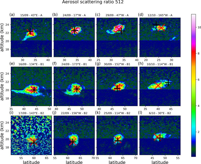
7114                      H. Lestrelin et al.: Smoke-charged vortices in the stratosphere: Australia 2020 vs. Canada 2017

rose up to 35 km (Khaykin et al., 2020) – an altitude not          To reduce the noise, a horizontal median filter with a 40 km
reached by tropospheric aerosols since the Pinatubo eruption.      width (121 pixels) was applied to the data. In order to sep-
Khaykin et al. (2020) conjectured that aerosol heating was         arate clouds from aerosols, we also used the Level 2 (L2)
essential in maintaining the structure and providing the lift.     total scattering aerosol coefficient at 532 nm which is avail-
In turn, the vortex created a confinement that preserved the       able at a 5 km resolution. Both daytime and night-time mea-
embedded smoke cloud from being rapidly diluted within the         surements were used. As the daytime measurements are nois-
environment.                                                       ier, they can only be used when the aerosol signal is strong
   Investigating the occurrence of such vortices after pre-        enough, mainly during the first few weeks following the re-
vious wildfires, in particular over the last 15 years during       lease of the plume.
which the required satellite instruments are available, is a          As in Khaykin et al. (2020), CALIOP inspection was the
natural extension of the work of Khaykin et al. (2020). As         first step in identifying the potential vortices. The L1 sec-
the strongest recorded wildfire of the last decade is the 2017     tions were systematically screened from 12 August to 15 Oc-
Canadian event that took place in British Columbia (Hanes          tober 2017, and those that contained isolated compact pat-
et al., 2019), this work revisits this case, which has already     terns above 11 km and were identified as aerosols by the L2
been documented in several studies (Khaykin et al., 2018;          product were selected. The location and size of the retained
Ansmann et al., 2018; Peterson et al., 2018; Yu et al., 2019;      patches were then determined by visually matching a rect-
Kloss et al., 2019; Baars et al., 2019; Torres et al., 2020). In   angular box to the observation, as illustrated in Fig. A1 in
particular, a stratospheric rise of up to 30 K d−1 in potential    the Appendix. It is usually very easy to see the boundaries of
temperature was diagnosed based on satellite observations by       the retained patches. In the next stage, the patches were asso-
Khaykin et al. (2018), and a compact smoke cloud at 19 km          ciated with the vortices detected as described in the follow-
over the Haute-Provence Observatory, southern France, on           ing, and further inspection rejected cases that corresponded
29 August 2017 was also reported in the same study. Another        to tails left behind by vortices (less than 20 % of those re-
goal of this work is to complement Khaykin et al. (2020) by        tained in the first stage).
expanding their diagnostics and interpretations on the 2020           Due to increased solar activity, CALIOP operations were
case.                                                              suspended between 5 and 14 September. This has been an
   This paper is structured as follows: Sect. 2 describes the      obstacle to establishing continuity based on CALIOP obser-
data and methods used in this work; Sect. 3 describes the          vations alone, but the tracking of the vortices filled that gap
new vortices found after the 2017 Canadian fire and their          as described below.
evolution, including a detailed discussion of previous results;
Sect. 4 describes the structure of the vortices based on the       2.2     Meteorological data
2017 Canadian case and the 2020 Australian case; and Sect, 5
offers conclusions.                                                2.2.1    Reanalysis

                                                                   To track the stratospheric wildfire vortices and diagnose their
2     Data and methods                                             dynamical structure, we used the ERA5 reanalysis (Hers-
                                                                   bach et al., 2020), which is the last-generation global at-
2.1    Satellite data from CALIOP                                  mospheric reanalysis of the European Centre for Medium-
                                                                   Range Weather Forecast (ECMWF). Khaykin et al. (2020)
Launched in April 2006, the Cloud-Aerosol Lidar and                used the ECMWF operational analysis and forecast instead;
Infrared Path Satellite Observation (CALIPSO) mission              however, both are based on the ECMWF Integrated Forecast
(Winker et al., 2010) hosts the Cloud-Aerosol Lidar with           System (IFS). In ERA5, the native horizontal resolution of
Orthogonal Polarization (CALIOP) onboard instrument – a            the IFS model is about 31 km, and it has 137 levels in the ver-
two-wavelength polarization lidar that performs global pro-        tical with spacing that varies from less than 400 m at 15 km
filing of aerosols and clouds in the troposphere and lower         to about 900 m at 35 km within the relevant altitude range of
stratosphere. We used the total attenuated 532 nm backscat-        this study. We used an extracted version of ERA5 with 1◦
ter Level 1 (L1) product in the latest available version, V4.10    resolution in latitude and longitude, at full vertical resolution
(Powell et al., 2009). The nominal along-track horizontal          and 3-hourly resolution. This choice was dictated by practi-
and vertical resolutions respectively are 1 km and 60 m be-        cal considerations in addition to the fact that this grid is able
tween 8.5 and 20.1 km and 1.667 km and 180 m between 20.1          to describe synoptic-scale features and that vortices do not
and 30.1 km. The L1 product oversamples the layers above           travel across more than a few grid points in 3 h.
8.5 km with a uniform horizontal resolution of 333 m. We              Khaykin et al. (2020) used temperature, ozone and vortic-
computed the scattering ratio by dividing the total attenuated     ity to investigate the structure of the vortices. In this study,
backscatter by the calculated molecular backscatter, follow-       we also used potential vorticity (PV). PV is a Lagrangian
ing Vernier et al. (2009) and Hostetler et al. (2006), and using   invariant for inviscid and adiabatic flows (Ertel, 1942); fur-
the meteorological metadata provided with the L1 product.          thermore, it provides a compact and complete picture of the

Atmos. Chem. Phys., 21, 7113–7134, 2021                                              https://doi.org/10.5194/acp-21-7113-2021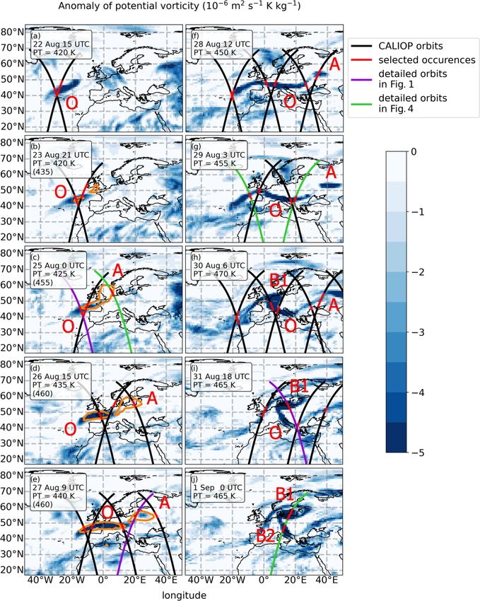
H. Lestrelin et al.: Smoke-charged vortices in the stratosphere: Australia 2020 vs. Canada 2017                              7115

balanced part of the flow (Hoskins et al., 1985). An inter-        before. This definition can be applied to any of the basic vari-
esting property of ERA5 is that its dynamical core preserves       ables of the model or to derived quantities like potential vor-
PV much better than previous reanalyses (Hoffmann et al.,          ticity. In ERA5, the assimilation increments can be calculated
2019). Although the ERA5 potential vorticity can be directly       on each day at 06:00 and 18:00 UTC. In order to diagnose
retrieved from the ECMWF archive on a given set of poten-          how the observations are forcing the vortices, we calculated
tial temperature levels, we instead recalculated it from the re-   the assimilation increments of temperature, vorticity, poten-
trieved vorticity, temperature and total horizontal wind fields    tial vorticity and ozone. Temperature and ozone determine
on model levels, in order to benefit from the full vertical res-   the radiances that are measured by space-borne instruments
olution offered by ERA5. For that purpose, we used the def-        and are also directly accessible from in situ instruments. On
inition of PV for the primitive equations in spherical coordi-     the contrary, potential vorticity cannot be directly retrieved
nates and model hybrid vertical coordinate η, which is given       from any instrument and is indirectly constrained (see be-
by                                                                 low). These three parameters are updated by the assimilation
                                                                  system in order to reduce the difference between observed
           ∂θ                                                     quantities (typically radiances but also deviations of the GPS
P = −g          f + ζη
           ∂p                                                      signal path) and simulated quantities (radiances that a satel-

       1 ∂θ ∂u           1 ∂θ ∂v
                                                                 lite flying “above the model” would see). It is tempting to
   +                −                   ,                    (1)   see the temperature assimilation increment as an additional
       a ∂φ η ∂p cos φ ∂λ η ∂p
                                                                   heating, but this is incorrect. The increment is calculated
where a is the radius of the Earth, λ is the longitude, φ is the   from an adjusted state, resulting from the iterations of the
latitude, g is the free-fall acceleration, ζη is the model level   assimilation, in which both temperature and motion respond
vertical component of the vorticity, f is the Coriolis param-      to the forcing from the observations. As wind observations
eter, (u, v) is the horizontal velocity, p is the pressure and     are much sparser than temperature observations, one would
θ is the potential temperature. The gradients are estimated us-    expect that analysis winds, and related quantities like poten-
ing centred differences on the retrieved longitude–latitude–η      tial vorticity, are more poorly constrained and, therefore, less
grid. See Eqs. (3.1.4) of Andrews et al. (1987) for an analo-      accurate than analysis temperatures. While this statement is
gous formula in barometric altitude coordinate.                    true to a large extent in the tropics, the temperature and wind
   While the formulation of PV in Eq. (1) is the most com-         fields are related through thermal wind balance in the mid-
monly used, it bears the disadvantage of a large background        latitudes. This equilibrium is enforced by the assimilation
vertical gradient, which proves inconvenient to track and          system which filters out the transient modes that deviate from
characterize structures along their ascent. To overcome this       it. Hence, thanks to this miracle of assimilation, assimilating
issue, we used the alternative formulation of Lait (1994), dis-    the temperature signal of the vortex is sufficient to recon-
cussed by Müller and Günther (2003):                               struct the whole thermal and dynamical field associated with
                                                                   the balanced structure (McIntyre, 2015).
           −                                                        It should be noted here that neither the ECMWF oper-
    θ
5=P               ,                                         (2)    ational analysis nor ERA5 assimilate aerosol observations.
    θ0
                                                                   The smoke plumes are totally absent from the IFS, where
where P is the Ertel PV,  = 4 in the Australian case and  =      stratospheric aerosols are only accounted for by the mean cli-
9                                                                  matological distribution during the periods of investigation,
2 in the Canadian case, and θ0 = 420 K. Compared with P ,
5 is still an adiabatic invariant and exhibits a reduced verti-    and it is only their dynamical vortical signature which is in-
cal gradient; thus, the vortices, characterized by anticyclonic    troduced in the model as described above.
5 anomalies, can be unambiguously distinguished during
their ascent. In each of the two cases, the value of  is chosen   2.2.3   Vortex tracking approach
to nearly cancel the background vertical gradient of 5, and it
depends on the large-scale vertical temperature profile char-      Once we caught the first occurrence of an isolated bubble of
acterized by larger (more positive) ∂T                             aerosols with CALIOP, we searched the ERA5 data for the
                                      ∂z in the Australian case
than in Canadian case (see Müller and Günther, 2003, for a         occurrence of a corresponding vortex that showed up as an
discussion regarding the choice of ).                             isolated pattern in the 5 and ozone maps. While Khaykin
                                                                   et al. (2020) used only relative vorticity to track the vortices
2.2.2   Assimilation increment                                     for convenience, we used both 5 defined from Eq. (2) and the
                                                                   ozone anomaly defined as the deviation with respect to the
ERA5 is constrained by observations over repeated 12 h as-         zonal mean at the same latitude and altitude. Tracking was
similation cycles. Over each cycle, the assimilation incre-        carried out every 6 h by following a local extremum within
ment is defined as the difference between the new analysis         a box of usually 12◦ in longitude, 5◦ in latitude and a range
and the first guess provided as a final stage of a free forecast   of at least 30 K of potential temperature in the vertical. Once
run of the model, initialized from the previous analysis 12 h      a vortex was caught, the box was moved forward in time to

https://doi.org/10.5194/acp-21-7113-2021                                            Atmos. Chem. Phys., 21, 7113–7134, 2021
7116                     H. Lestrelin et al.: Smoke-charged vortices in the stratosphere: Australia 2020 vs. Canada 2017

the step n + 1 according to the vortex motion between steps       titude of 12 km just above the tropopause. In the following
n−1 and n. In very few instances, the tracking was guided by      days, this anomaly developed vertically and connected with
reducing the size of the box. In particular, this was needed at   the bubble O location as identified from CALIOP (see an-
the formation of a vortex, or during a breaking event, when       imation in Sect. S2 of the Supplement). On 17 August, as
it split into two parts, or in the final stage when one of the    it crossed Hudson Bay, it exhibited a well-developed intru-
methods lost the track before the other.                          sion that reached 14 km in the PV longitudinal and latitudi-
                                                                  nal section. As seen in the animation, this intrusion, while
                                                                  still rising, was subsequently stretched by the vertical shear
3     A new occurrence: Canada 2017                               and split into an upper and lower part by 19 August: the upper
                                                                  part was isolated in the stratosphere at about 15 km, whereas
3.1    General description
                                                                  the lower part near the tropopause was further stretched and
Although the 2017 Canadian fire started in June (Hanes et al.,    disappeared. The upper part, which was associated with bub-
2019), it was not until 12 August to early on 13 August that      ble O, was tracked in the ERA5 ozone and PV fields and from
the fire reached an intensity such that a large PyroCb devel-     CALIOP until the end of August (Fig. S1 in the Supplement).
oped and reached the lower stratosphere, leaving a smoke          As it crossed the Atlantic, it became trapped inside a trough
plume that could be followed by satellite sensors (Khaykin        on 20 August and then travelled with it until it reached the
et al., 2018; Peterson et al., 2018; Torres et al., 2020). From   European coast. Due to the wind shear prevailing in the as-
the inspection of the scattering ratio along CALIPSO orbits,      sociated jet, vortex O elongated in latitude across the isen-
we found our first distinctly isolated smoke bubble on 16 Au-     tropes (see the animation) until it became split into the three
gust at 09:38 UTC and 12.6 km altitude over the north of          parts, A, B1 and B2, over western Europe, as described in the
Canada (63◦ N and 102◦ W), where the tropopause altitude          next section.
was 11 km. Two days after the first evidence of the presence         This early stage is also described in great detail by Torres
of smoke in the stratosphere (Peterson et al., 2018; Torres       et al. (2020). This previous study shows that the whole smoke
et al., 2020). In the following days and until the CALIOP         cloud is shaped like a V, on 20 August, by its passage in the
interruption on 4 September, we could track this cloud, la-       trough, resulting in a double maximum tilted pattern in the
belled as bubble O, and its offspring almost every day. Fig-      section by CALIOP. This pattern is recovered in the ERA5
ure 1 shows several typical patterns during that period.          PV pattern (freeze the animation in Sect. S2 of the Supple-
   As indicated by the longitudes in Fig. 1, bubble O moved       ment on the same date), and our tracking actually follows the
eastward across the Atlantic. During the early days, it was       highest of the two maxima.
captured each day by at most two CALIPSO orbits (one day
orbit and one night orbit), with the adjacent orbits only show-   3.3   Horizontal and vertical splitting of vortex O into its
ing filamentary non-compact structures that could be eas-               offspring
ily distinguished. The bubble rose rapidly reaching 18 km
by 25 August (i.e. an ascent rate larger than 0.5 km d−1 ).       Figure 3 displays the series of events that led, over the period
One surprising feature is that once it had reached the Eu-        from 22 August to 1 September, to the splitting of vortex O
ropean coast by 27 August, several bubbles could be tracked       into its three offspring, which were subsequently followed
on multiple close orbits or even, exceptionally, on the same      over 1.5 months. We display the CALIPSO orbits that in-
orbit. As we shall see in the following, this corresponds to      tersect the vortex cores as well as those that intersect their
the splitting of bubble O into several offspring that we label    tails. The presence of a smoke bubble or patch detected by
as A, B1 and B2 for which several views are shown in Fig. 1.      CALIOP along an orbit is shown as a red segment. For all
Another issue came soon after as CALIOP operations were           orbits, we see that there are bubbles or patches that match
suspended for the period from 5 to 14 September due to in-        each of the intersections with the tracked low-PV regions.
creased solar activity. When CALIOP observations resumed          The sequence begins on 22 August (Fig. 3a) with the elon-
after 14 September, the A, B1 and B2 bubbles that were now        gated structure of vortex O that emerged at 420 K on the east-
located at 20 km or above could be found again, over central      ern flank of the trough within which it crossed the Atlantic.
Asia for A and over the Pacific for B1 and B2, and they were      The elongation was due to the intense vertical shear in the
followed during their subsequent journey until mid-October.       jet stream. The formation of vortex A is already shown by
Figure 2 shows a selection of views during that period.           the “rolling up” pattern on the north-east end of vortex O.
                                                                  On 23 August (Fig. 3b), the pattern of vortex A is lost at
3.2    Early evolution                                            the 420 K level but is now visible at the 435 K level. A to-
                                                                  tal of 2 d later (Fig. 3c), vortex A was a developed structure
The smoke bubbles were attributed to vortices based on the        reaching 60◦ N at the 455 K level, and it was overflown by
ERA5 reanalysis which were available throughout their life        CALIPSO (Fig. 4a). At the same time, vortex O maintained
cycles. Starting on 14 August, a kernel of almost zero PV         a core near 45◦ N (Fig. 1d). In the following days, 26 and
and low ozone could be found at 72◦ N, 115◦ W and an al-          27 August (Fig. 3d and e respectively), vortex A fully sepa-

Atmos. Chem. Phys., 21, 7113–7134, 2021                                             https://doi.org/10.5194/acp-21-7113-2021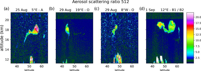
H. Lestrelin et al.: Smoke-charged vortices in the stratosphere: Australia 2020 vs. Canada 2017 7117
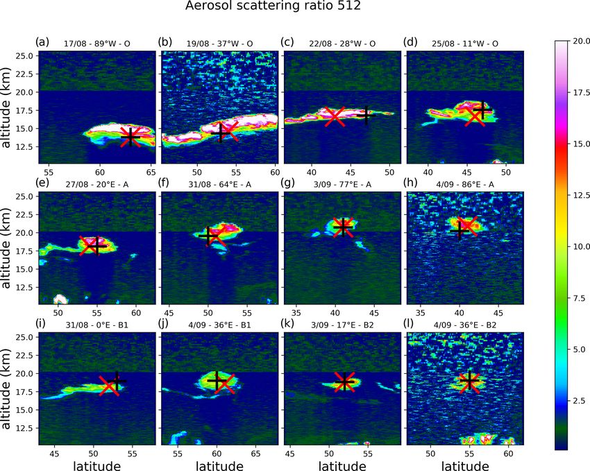
Figure 1. Selection of along-track sections of the CALIOP scattering ratio profiles during the first observation period until 4 September
2017. Panels (a–d) show sections of bubble O at four times. Panels (e–h) show four sections of bubble A after its separation from bubble O.
Panels (i–l) show two sections of bubble B1 after its separation from bubble O (i, j) and two views of bubble B2 that continues the track of
bubble O after 1 September 2017 (k, l). In each panel, the black and red crosses show the orbital plane projection of the corresponding vortex
centre according to the Lait PV 5 and ozone tracking in ERA5 data respectively. For each panel, the longitude indicated in the title is that of
the CALIPSO orbit at the centre of the bubble.
rated from vortex O as it moved eastward and rose (Fig. 1e). 3.4 Late evolution
On 28 and 29 August (Fig. 3f and g respectively), vortex A
moved away while vortex O was re-elongated and started to During the observation period that followed the recovery of
split into a western (Fig. 4b) and an eastern part (Fig. 4c). The CALIOP after 15 September until mid-October, almost all
vertical structure of vortex A on 28 August in another reanal- observations of compact smoke bubbles at 20 km and above
ysis is briefly shown in Fig. 16 of Allen et al. (2020). On 30 could be attributed to one of the vortices, A, B1 or B2. We
and 31 August (Fig. 3h and i respectively), the western part discarded other observations of smoke patches that were un-
separated while the eastern part folded itself and separated der the shape of filaments. A number of these filaments be-
into two more parts that provided vortex B1 as the north- longed to tails left behind by the bubbles along their paths.
ern component (Fig. 1) and vortex B2 as the southern com- As in Fig. 1, the location of the ERA5 vortex centre is shown
ponent (essentially a continuation of vortex O), which were using a cross in each panel of Fig. 2. The locations of the
both seen on the same CALIOP overpass on 1 September smoke bubble centres are shown as square marks in Fig. 5
(Figs. 3j and 4d). The B1 and B2 vortices fully separated in which describes the trajectory of vortex A, and the bars in-
the following days while rising and starting to move slowly dicate the latitudinal and altitudinal extent of the bubble. A
eastward. The western component could also be followed un- perfect match with respect to the horizontal location is not
til 4 September, accompanied by patches seen by CALIOP; expected, as there is no reason for the CALIPSO orbit to
however, it remained below 460 K and could not be linked cross the vortex centre every time. Nevertheless, we see very
to any structure seen from CALIOP after 15 September with good agreement between the ERA5 trajectory and the lo-
any certainty. cation of the 27 smoke bubbles seen by CALIOP that are
attributed to vortex A, and the same holds for vortices B1
https://doi.org/10.5194/acp-21-7113-2021 Atmos. Chem. Phys., 21, 7113–7134, 2021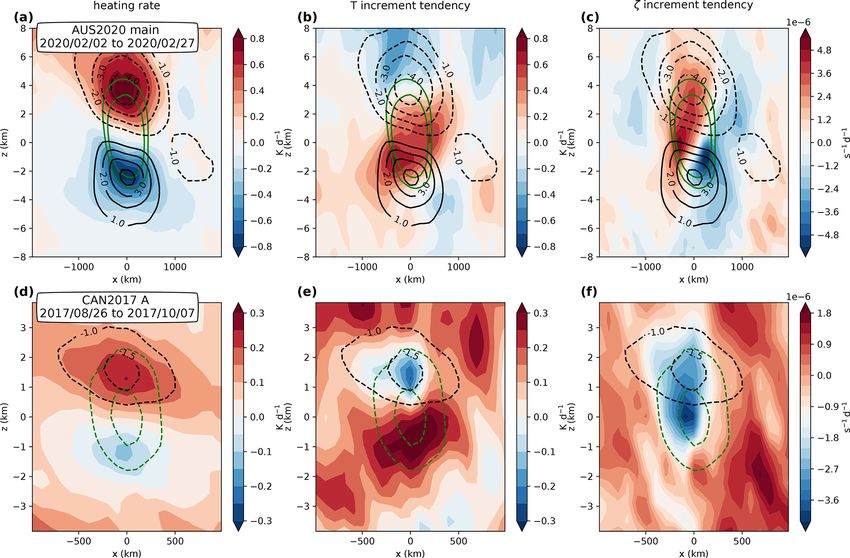
7118                      H. Lestrelin et al.: Smoke-charged vortices in the stratosphere: Australia 2020 vs. Canada 2017

Figure 2. Same as Fig. 1 but during the second observation period after 15 September 2017, showing four sections of bubbles A (a–d),
B1 (e–h) and B2 (i–l).

and B2 (Figs. S2 and S3 in the Supplement), both with 21 at-        tant to sense the thermal signature of the vortex (Khaykin
tributions. The evolution of vortices A, B1 and B2 is also          et al., 2020). The detection of ozone is less affected, as it
available as animations in Sect. S3 of the Supplement. Vor-         also uses instruments such as the Global Ozone Monitoring
tex A was the first to separate from the mother vortex, vor-        Experiment-2 (GOME-2) (Khaykin et al., 2020) that oper-
tex O, on 22 August, and it first moved eastward until it           ate in the ultraviolet range. The fact that the PV signature
reached central Asia on 1 September at a latitude of 55◦ N          re-intensifies as soon as the vortex is over the Atlantic sup-
and a longitude of 60◦ E. It then became trapped in the re-         ports this hypothesis. During the last stages of the vortex, by
gion of slow motion that extends between the two centres of         mid-October, we also see a premature loss of the PV signal,
the Asian monsoon anticyclone (AMA) and started to drift            whereas the ozone signal is still detectable and can be de-
slowly southward while staying at about the same longitude          tected beyond the end of our tracking. This pattern is shared
and maintaining its ascent rate. A week later, it reached 35◦ N     by the two other vortices, B1 and B2, and it differs from the
where it was caught in the easterly circulation and started         2020 case where an effect such as this is not observed for
to move westward, crossing Africa and continuing its path           any of the vortices studied by Khaykin et al. (2020). Besides
which could be tracked until the western Pacific. Figure 6          the increase in the IASI fleet, from two to three instruments,
shows a composite image of successive images of the local-          we do not see any drastic change in the observation system
ized ozone hole from ERA5. It was easier to track the vortex        between the two events.
using the ozone field than the PV. In particular, the PV signal        While vortex A was completing its transition to the trop-
almost vanished as it passed over Africa (see the vortex A          ics, the two other vortices, B1 and B2, travelled eastward
animation in the Supplement), whereas the ozone signature           within the westerly flow on the northern side of the AMA,
was always very clear. We attribute the near disappearance          both reaching the Pacific on 18 September. Vortex B1 crossed
of the PV signal to the strong infrared emissivity of the Sa-       the Pacific at mid-latitude and was lost near Hudson Bay af-
hara that limits the sensitivity of the Infrared Atmospheric        ter having crossed most of North America by 14 October.
Sounding Interferometer (IASI) sounders, which are impor-           Vortex B2, which travelled at a higher latitude, completed a

Atmos. Chem. Phys., 21, 7113–7134, 2021                                               https://doi.org/10.5194/acp-21-7113-2021
H. Lestrelin et al.: Smoke-charged vortices in the stratosphere: Australia 2020 vs. Canada 2017                                          7119

Figure 3. Sequence of PV charts showing the splitting of vortex O into vortices A, B1 and B2. The map is plotted on the potential temperature
surface corresponding to the core of vortex O or its continuation B2 in the ERA5 tracking. The orange lines are plotted at the isentropic level
of vortex A, specified within parenthesis, and show the contour of −2 PVU (1 PVU = 10−6 K m2 kg−1 s−1 ) for vortex A. The black, green
and purple lines show the intersecting orbits of CALIPSO, and the red segments show the parts of the orbits occupied by the bubble (only the
bubble core extent is displayed here). The maps are plotted at the hour that best matches the selected CALIOP occurrences. The purple orbits
are those corresponding to the sections shown in Fig. 1; the green orbits are those corresponding to the sections shown in Fig. 4. Daytime
and night-time orbits are used: the daytime orbits run from south-east to north-west, whereas the night-time orbits run from north-east to
south-west. Starting from 1 September, the remainder of vortex O is relabelled as B2.

full round-the-world journey during the same period and was               up to 23 km for vortex A and to 21 km for vortices B1 and B2
lost over central Asia by 11 October. Figure 7 summarizes the             (altitudes of the core).
trajectories of vortices O, A, B1 and B2 from their formation
to their loss. The total recorded paths of the four vortices are
13 000, 42 400, 28 500 and 33 400 km respectively. They rose

https://doi.org/10.5194/acp-21-7113-2021                                                    Atmos. Chem. Phys., 21, 7113–7134, 2021
7120                        H. Lestrelin et al.: Smoke-charged vortices in the stratosphere: Australia 2020 vs. Canada 2017

Figure 4. Selection of four CALIOP scattering ratio sections of the smoke bubbles along the orbits shown in green in Fig. 3: (a) daytime
section of bubble A on 25 August, (b) east night-time and (c) west daytime sections of elongated bubble O on 29 August, and (d) night-time
double section of bubbles B1 (at ∼ 55◦ N) and B2 (at ∼ 45◦ N) on 1 September.

                                                                          – The ascent rate was the strongest during the initial stage
                                                                            of vortex O when it rose from its origin just above the
                                                                            tropopause. Previous studies based on CALIOP or limb-
                                                                            sounding instruments have reported an ascent rate using
                                                                            the upper envelop of the bubble. Yu et al. (2019) re-
                                                                            ported an ascent from 14 to 20 km from 15 to 24 August,
                                                                            and Khaykin et al. (2018) reported an ascent of 30 K d−1
                                                                            in potential temperature (or 3 km d−1 ) between 16 and
                                                                            18 August. We used the centroid of the PV and O3
                                                                            anomalies to define the ascent and found (see Fig. S1
                                                                            in the Supplement) that vortex O ascended from 12 to
                                                                            17 km between 14 and 24 August, which is consistent
                                                                            with Yu et al. (2019), but we found no trace of a faster
                                                                            ascent. From 24 to 31 August, vortices O and A (see
                                                                            Fig. 5) climbed by 2 km, and vortex A maintained this
                                                                            rate until 8 September when it reached 21 km. It took
                                                                            1 more month to reach the maximum altitude of 23 km,
                                                                            whereas B1 and B2 reached 21 km within the same time
                                                                            period. In the initial stage, Torres et al. (2020) claimed
                                                                            an ascent of 20 K d−1 on 14 August when the smoke
                                                                            bubble was detected in the stratosphere by CALIOP for
Figure 5. The trajectory of vortex A tracked from the ERA5                  the first time. However, the assumption of a tropopause
fields of PV (orange) and ozone (green): (a) the trajectory in the          crossing between 13 and 14 August is questionable, as
longitude–latitude plane; (b–d) latitude, longitude and altitude as a       the sections of CALIOP through the smoke cloud were
function of time respectively. The green curves mostly mask the or-
                                                                            on its periphery on 13 August, as shown by Fig. 1d
ange curves as they almost exactly coincide. The boxes show the lo-
                                                                            of Torres et al. (2020) (even adding the missing night
cation of the smoke bubble according to CALIOP during CALIPSO
overpasses, and the bars indicate the range of the bubble in latitude       orbit). Therefore, it is equally plausible that the pyro-
and altitude.                                                               convective event directly injected smoke into the strato-
                                                                            sphere without requiring large internal radiative heating.
                                                                          – Peterson et al. (2018) noticed the formation of vor-
                                                                            tex O from CALIPSO and Ozone Mapping and Profiler
3.5    Comparison with previous studies                                     Suite (OMPS)/Suomi National Polar-orbiting Partner-
                                                                            ship (SUOMI NPP) overpasses on 14 August in north-
Several previous studies have discussed the various stages of               ern Canada. Both Khaykin et al. (2018) and Peterson
smoke cloud evolution described above, although none have                   et al. (2018) reported that the first smoke patches had
made the link with a PV structure. Thus, a number of com-                   reached Europe by 19 August, and they were observed
ments are in order here:                                                    by a ground lidar station in central Europe on 22 Au-

Atmos. Chem. Phys., 21, 7113–7134, 2021                                                   https://doi.org/10.5194/acp-21-7113-2021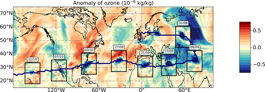
H. Lestrelin et al.: Smoke-charged vortices in the stratosphere: Australia 2020 vs. Canada 2017                                            7121

Figure 6. Sequence of ozone anomalies along the trajectory of vortex A for selected dates from 31 August to 11 October. The background is
the mean ozone anomaly over this period at 460 K. For each selected day, the box shows the ozone anomaly on that day at 00:00 UTC at the
level of the vortex centroid according the ozone anomaly tracking, reported along the blue line.

Figure 7. Trajectories of the vortices based on the low-ozone anomaly from the ERA5 analysis at a 6 h sampling resolution. The colour
gradient along each trajectory shows the time evolution of the vortices. We follow vortex O from 14 July 2017 until 31 August; it is then
relabelled as vortex B2, and we follow its course until 11 October. Vortex A separates from vortex O on 22 August and is followed until
18 October. Vortex B1 separates from vortex O on 27 October and is followed until 14 October. Panel (c) shows the ascent in both altitude
(left axis and lower set of curves) and potential temperature (right axis and upper set of curves). The crosses cover the part of each trajectory
where CALIOP was not available.

https://doi.org/10.5194/acp-21-7113-2021                                                      Atmos. Chem. Phys., 21, 7113–7134, 2021
7122 H. Lestrelin et al.: Smoke-charged vortices in the stratosphere: Australia 2020 vs. Canada 2017
gust (Ansmann et al., 2018; Baars et al., 2019). These 4 Structure of the vortices in 2020 and 2017
patches followed a northern route faster than that of
vortex O and were seen as filamentary structures by 4.1 Composite analysis of the vortices in ERA5
CALIOP. Their forefront reached Asia by 24 August.
By 29 August, a thick layer of smoke with an aerosol Here, we investigate the structure of the vortices by the mean
optical depth of 0.04 was seen from a lidar in south- of a composite analysis. The dynamical fields surrounding
eastern France at 19 km (Khaykin et al., 2018), corre- the vortex centroids were re-gridded regularly in Cartesian
sponding to the passage of vortex O in the vicinity. Ac- geometry in the horizontal and in log-pressure altitude (An-
cording to our tracking, the lidar saw the tail connect- drews et al., 1987) in the vertical, within a moving frame that
ing vortex O to vortex B1 during the course of sep- follows the centroids’ ascent and horizontal displacement. As
aration (see Sect. 3.3). Bourassa et al. (2019) noticed in Khaykin et al. (2020), the composite model fields were
the southward motion of vortex A over Central Asia then averaged in time to generate a composite analysis that
but interpreted it as a split of the plume over this re- filters out noise and variability unrelated to the vortices. This
gion on 1 September; however, the separation actually procedure also removes short-term vacillations (see Khaykin
occurred 1 week before. It is tempting to see a trace et al., 2020; Allen et al., 2020) which are a common property
of vortex A in the OMPS signal at 30◦ N above 20 km of vortices in shear flow (e.g. Tsang and Dritschel, 2015),
during September in Fig. 1 of Bourassa et al. (2019) thereby enabling us to emphasize the mean structure of the
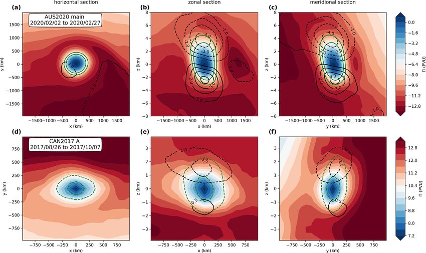
and in the Stratospheric Aerosol and Gas Experiment III vortex. Figure 8 depicts the composite of Lait PV 5 (defined
(SAGE III) low-latitude signal above 20 km during Oc- in Eq. 2) and the temperature anomaly following vortex A
tober in Fig. 1d of Kloss et al. (2019). Bourassa et al. (Fig. 8d–f) and the main Koobor vortex (Fig. 8a–c) gener-
(2019) were able to track smoke patches until January ated by the 2020 Australian fires and tracked by Khaykin
2018, and the global signature at altitudes up to 24 km et al. (2020). In the natural coordinates, without expanding
persisted until summer 2018 (Kloss et al., 2019). the vertical direction, both vortices appear as isolated pan-
cakes of anomalous anticyclonic Lait PV (i.e. negative in
– Using several satellite instruments and transport calcu- the Northern Hemisphere and positive in the Southern Hemi-
lations, Kloss et al. (2019) found the transport of smoke sphere). The analysed temperature anomaly consists of a ver-
patches to the tropics taking place on the eastern south- tical dipole surrounding the PV monopole with a negative
ward branch of the AMA, but they excluded transport temperature anomaly above and a positive temperature be-
across the AMA which is what we observe for vor- low it, whose centres are located on the upper and lower
tex A. These authors focused their work on the events edges of the Lait PV distribution. As noted by Khaykin et al.
of the last week of August and on levels below 20 km. (2020), this relationship between temperature stratification
The transition of vortex A occurred in early September and vorticity is qualitatively consistent with the thermal wind
and it was already above 20 km. The smoke layer that balance and is characteristic of anticyclonic vortices in the
Kloss et al. (2019) subsequently followed in the tropics quasi-geostrophic (QG) equations (Dritschel et al., 2004) as
includes the effect of vortex A. well as of balanced anticyclones in the full primitive equa-
tions (e.g. Hoskins et al., 1985). In the case of the smoke-
– Baars et al. (2019) showed interesting evidence of charged vortices investigated here, it turns out that their in-
aerosol patches over Europe and the Mediterranean area tensity is slightly beyond that of the typical geostrophic flow.
reaching 23 km by mid-September 2017 and again in The typical Rossby number of the structure can be expressed
mid-December 2017. Although unstated, they do not as follows:
expect the second patches to be the remnant of the first.
They instead provide an explanation based on a circuit U ζ
Ro = ' , (3)
identified by Kloss et al. (2019), where smoke patches f Lh f
were injected into the tropics in early September. The where U is the maximum horizontal wind speed, Lh is the
smoke then rose slowly to higher levels in the trop- horizontal length scale (defined as the diameter of the ring of
ics and came back to the mid-latitudes carried by the the local wind speed maximum at the altitude of the centroid
Brewer–Dobson meridional circulation. There is, how- and estimated in the west–east direction) and ζ = U/Lh is
ever, a hole in the reasoning of Baars et al. (2019): the average relative vorticity. Ro is about 0.06 in the 2017
the tropical rise is reported to reach 21 km by March case and 0.35 for 2020. While the Rossby number is beyond
2018, whereas the aerosols supposedly blown away by the typical QG regime (Ro < 0.1) in 2020, the aspect ratio α,
the Brewer–Dobson are found at 23 km over Europe in defined as
December 2017. It is now clear that the missing piece Lz
of the puzzle is provided by vortex A which reached α= ' 5 × 10⁻³ (4)
Lh
23 km by late September (with a top at 24–25 km) and
left a tail along its path. (where Lz is the vertical extent of the contour of vorticity
at maximum wind speed at the horizontal location of the
Atmos. Chem. Phys., 21, 7113–7134, 2021 https://doi.org/10.5194/acp-21-7113-2021H. Lestrelin et al.: Smoke-charged vortices in the stratosphere: Australia 2020 vs. Canada 2017 7123
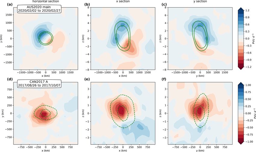
Figure 8. Time-averaged composite sections of Lait PV 5, in PVU (1 PVU = 10−6 K m2 kg−1 s−1 ), following two selected smoke-charged
vortices, the main Koobor vortex from the 2020 Australian wildfires described in Khaykin et al. (2020) (a–c) and vortex A introduced in this
paper (d–f). Panels (a) and (d), (b) and (e), and (c) and (f) show the respective horizontal, zonal and meridional sections through the centroid
of the vortex. The green lines are contours of anticyclonic vertical vorticity (corresponding to 3 × 10⁻⁵ and 5 × 10⁻⁵ s−1 for panels a–c, and
−1.5 × 10⁻⁵ and −2.5 × 10⁻⁵ s−1 for panels d–f). The black contours are the temperature anomaly with respect to the zonal mean. Note
that the horizontal and vertical ranges displayed are reduced by a factor of 2 for vortex A.
f
vortex centroid), obeys the stratified QG scaling α ' N in Burger number Bu ∼ 1, as typically encountered in geophys-
both cases, despite the 2017 vortex A being about 2.3 times ical flows. Furthermore, most vortices in Table 1 obey the QG
smaller in volume than its gigantic 2020 counterpart. aspect ratio, so that they are quasi-spherical (see Fig. 8) when
To further investigate the dynamical regime in which the the vertical coordinate is stretched by a factor N f . This obser-
identified vortices evolve (or their representation in the IFS), vation is consistent with numerical studies of ellipsoidal vor-
Table 1 presents their typical sizes; their amplitude charac- tices, which have demonstrated the higher stability of quasi-
terized by the Rossby number Ro and the Froude number, spherical vortices (Dritschel et al., 2005) and the tendency of
aspherical vortices hto relax towards sphericity in the stretched
U N
i
Fr = ; (5) coordinate system x, y, f z (Tsang and Dritschel, 2015).
Lz N
Contrary to its aspect ratio, the magnitude of the vor-
and the absolute vorticity amplitude at the vortex centroid tex perturbation is case-dependent and does not necessarily
normalized by f , fit in the classical QG scaling, thereby contrasting with the
synoptic-scale circulation. Indeed, typical vortex-averaged
ζa ζ +f
= , (6) Rossby numbers range from 0.06 up to 0.35, a range simi-
f f lar to observed mesoscale and sub-mesoscale oceanic eddies
which measures the inertial (in)stability of the flow. It should (e.g. Le Vu et al., 2017). For the intense 2020 Koobor vor-
be noted that despite the similarity, ζfa is not redundant with tex, the maximum vorticity in the vortex core is on the verge
Ro defined in Eq. (3) and characterizes the extremum rather of inertial instability or even slightly beyond its threshold for
than the structure average of the vorticity. linear flows (Hoskins, 1974), as can be seen from the positive
Keeping the limited vertical and horizontal resolution of 5 values in Fig. 8 (see also the small negative values of ζfa
the IFS in mind, it can be noticed that the Froude and in Table 1). This property was maintained over 1.5 months
Rossby numbers are always of the same order, leading to a from the formation of the Koobor vortex to its first breaking
https://doi.org/10.5194/acp-21-7113-2021 Atmos. Chem. Phys., 21, 7113–7134, 20217124 H. Lestrelin et al.: Smoke-charged vortices in the stratosphere: Australia 2020 vs. Canada 2017
f
Table 1. The horizontal diameter (Lh ), vertical depth (Lz ), aspect ratio (α), QG aspect ratio imposed by the environment ( N ), Rossby
number, Froude number and maximum vorticity ( ζfa ) of the six smoke-charged pancake vortices originating from the Canadian (2017) and
Australian (2020) wildfires. The 2020 Koobor vortex was long-lasting and is decomposed into two periods here.
f ζa
Name Geographic origin Period considered Lh (km) Lz (km) 103 α 103 N Ro Fr f
Koobor Australia 7–27 Jan 2020 784 6.1 7.8 6.6 0.35 0.30 0.03
Koobor Australia 2–27 Feb 2020 784 6.1 7.8 5.8 0.33 0.25 −0.09
2nd Vortex Australia 18–27 Jan 2020 588 3.8 6.5 6.6 0.35 0.35 −0.12
3rd Vortex Australia 20 Jan–7 Feb 2020 588 7.7 13.1 7.9 0.10 0.06 0.72
Vortex A Canada 26 Aug–7 Oct 2017 686 3.5 5.1 4.8 0.06 0.06 0.6
Vortex B1 Canada 27 Aug–7 Oct 2017 588 4.5 7.6 6.2 0.12 0.10 0.56
Vortex B2 Canada 1 Sep–7 Oct 2017 490 3.8 7.8 7.0 0.11 0.09 0.6
(see Fig. S4 in the Supplement). Although it is not clear how – a failure to reproduce the observed ascent of the struc-
realistic the ECMWF vortices are, their amplitude is likely ture at about 6 K d−1 in potential temperature – on the
underestimated as they are forced by data assimilation and contrary, the modelled anticyclones tend to remain at
the stand-alone model does not simulate them. Therefore, we constant θ ;
cannot generally conclude on the amplitude of the perturba-
– a decay of the vorticity anomaly within 1 week, whereas
tions, in particular that of the smaller Northern Hemisphere
the observed vortex survives for more than 3 months.
vortices. Nevertheless, the 2020 cases demonstrate that the
vorticity anomaly may reach the threshold for inertial insta- This suggests that data assimilation of observed temper-
bility at which it likely saturates. ature and ozone profiles is a necessary ingredient to both
Related to their different magnitudes, the vortices also the ascent and the maintenance of the vortex in the model,
have distinct impacts on their immediate surroundings, as can whereas some physical or spurious processes act to dissipate
be identified in Fig. 8. While the 2020 Koobor vortex was the structure. In the atmosphere, it is assumed that the forc-
strong enough to generate a significant cyclonic PV anomaly ing is exerted by radiative heating through solar absorption
eastward of the vortex centroid which rolls up around it on its by black carbon aerosols within the smoke (Yu et al., 2019).
northern edge, no such signature can be distinguished around Thus, increments are expected to be a substitute in the analy-
vortex A. In a zonal plane, the 2020 negative PV patch has sis system for the diabatic tendency maintaining the vortices,
diameter comparable to the Koobor vortex but a reduced as wildfire smoke is missing from the model.
magnitude. The existence of this negative anomaly can be
attributed to the equatorward advection of cyclonic PV on 4.2.1 Temperature and vorticity tendencies
the eastern flank of Koobor and is likely responsible for the
Figure 9a and d depict the average composite of the ERA5
equatorward beta-drift (Lam and Dritschel, 2001) undergone
total heating due to physics calculated over the forecast. This
by Koobor during its ascent.
field is dominated by the longwave radiative heating com-
Finally, for completeness, two further remarks should be
ponent as the shortwave absorption by the smoke is miss-
made. First, the reader should note that the vertical temper-
ing from the IFS. The dominant feature shown by Fig. 9 is a
ature dipole is slightly asymmetric with a larger magnitude
damping of the temperature anomaly T 0 with respect to the
of the negative temperature anomaly. Second, Fig. 8c shows
radiative equilibrium temperature which can be cast into a
that the vertical axis of Koobor exhibits on average a small
Newtonian relaxation as follows:
tilt with altitude, being slanted along the south–north direc-
tion, which is perpendicular to the prevailing background DT 0 T0
'− , (7)
shear. This property is a common characteristic of vortices Dt τrad
undergoing shear (Tsang and Dritschel, 2015) and is related where τrad is the radiative damping rate. Figure 9 suggests
to the temporal vacillations of Koobor described by Allen τrad ' 6–7 d. This is consistent with the lifetime of the struc-
et al. (2020) and also seen in Fig. 6 of Khaykin et al. (2020). ture in the ECMWF forecast which is about 1 week (Khaykin
et al., 2020), suggesting that radiative dissipation plays a ma-
4.2 Diagnosing diabatic tendencies jor role in the decay of the vortex in the model but also in the
real atmosphere.
By comparing the 2020 Koobor vortex in the ECMWF anal- However, as the model itself cannot sustain the vortices,
yses and model forecasts, Khaykin et al. (2020) showed sys- it comes down to data assimilation to maintain the struc-
tematic shortcomings of the free-running model with respect ture. Khaykin et al. (2020) demonstrated that the IFS ex-
to the analysis, namely tracts information from the thermal signature and the ozone
Atmos. Chem. Phys., 21, 7113–7134, 2021 https://doi.org/10.5194/acp-21-7113-2021H. Lestrelin et al.: Smoke-charged vortices in the stratosphere: Australia 2020 vs. Canada 2017 7125 Figure 9. Time-averaged composite sections of the ERA5 total heating rate (a, c), increment-induced temperature (b, e) and vorticity ten- dency (c, f) following two selected smoke-charged vortices, the major vortex from the 2020 Australian wildfires described in Khaykin et al. (2020) (a–c) and vortex A (d–f). The green lines are contours of anticyclonic vertical vorticity (corresponding to 3 × 10⁻⁵ and 5 × 10⁻⁵ s−1 for panels a–c, and −1.5 × 10⁻⁵ and −2.5 × 10⁻⁵ s−1 for panels d–f). The black contours are the temperature anomaly with respect to the zonal mean. Note that the displayed horizontal range is reduced by a factor of 2 for vortex A. anomaly detected by satellite instruments. The temperature to the composite vortex, the composite vorticity and temper- increments are shown in Fig. 9b and e. In contrast to the ature increment tendencies exhibit the structure of a balanced heating rates, which are instantaneous forcing of the tem- vortex: the 2017 anticyclonic ζ tendency monopole is sand- perature by physical processes, the temperature increments wiched between the two extrema of the temperature incre- result from the balanced dynamical response of the tempera- ment dipole, whereas the tripole of the T increment alternates ture field to the forcing induced by the discrepancy of mea- with the two layers of vorticity anomalies in 2020. Overall, sured radiances with respect to their estimated values in the the T and ζ patterns of the 2020 assimilation increment are assimilation procedure. Hence, the temperature pattern does qualitatively consistent with the expected effect of localized not match the observed aerosol bubble co-located with the heating in a rotating atmosphere (as sketched in Fig. 10 of vortex which would be expected for the shortwave aerosol Hoskins et al., 2003). absorption; rather, it exhibits a multipolar structure, essen- Together with the apparently balanced vortex structure of tially oriented vertically. In the 2017 case with a limited ver- the increments, the similarity to the theoretical response in tical ascent rate, the T increment vertical dipole mainly can- Hoskins et al. (2003) suggests that potential vorticity (or Lait cels the radiative damping. In 2020, it is rather a tripole that PV) is the appropriate field to consider for a more straight- enables the maintenance and the ascent of the dipolar tem- forward interpretation of the increments in terms of missing perature anomaly structure. diabatic processes. This is the focus of the next subsection. Due to this dynamical adjustment, temperature is not the only field incremented via data assimilation. Figure 9c and f show the increments of relative vorticity ζ . They contribute again to the maintenance (2017 case) and the ascent and maintenance (2020 case) of the vortices. Moreover, similarly https://doi.org/10.5194/acp-21-7113-2021 Atmos. Chem. Phys., 21, 7113–7134, 2021
7126 H. Lestrelin et al.: Smoke-charged vortices in the stratosphere: Australia 2020 vs. Canada 2017
Figure 10. Same as Fig. 8 but for Lait PV increments.
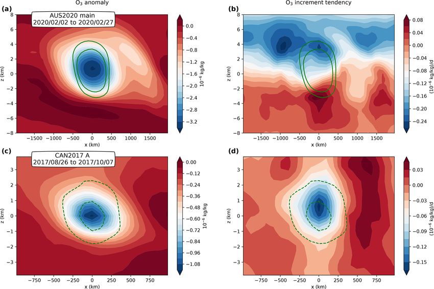
4.2.2 Lait PV and ozone tendencies due to assimilation as in the middle of January 2020 (see Fig. B1), emphasizing
increments that the inclination of the increment dipole is due to the back-
ground wind shear rather than the local wind at the altitude
of the vortex.
Composite time-averaged increments of Lait PV 5 are pre- The different patterns of Lait PV 5 (Fig. 8) and its in-
sented in Fig. 10. As stressed above, 5 increments result crement (Fig. 10) around the vortex are mimicked in the
from a combination of both temperature and vorticity and ozone field, as shown in Fig. 11. As described above, the
appear due to the implicit incorporation of temperature ob- ascending anticyclonic vorticity anomalies are accompanied
servations into an approximately dynamically balanced re- by negative ozone anomalies (Fig. 11a, c). Compared with
sponse by the 4D-Var scheme used in ERA5. Figs. 8 and 10, Fig. 11 shows that the patterns of the ozone
Contrary to the mean vortex structure in Fig. 8, we notice a anomaly bubble and its increment are very similar to those
stark contrast between the Northern Hemisphere and South- of 5. We note that the magnitude of the increments may
ern Hemisphere vortices. In the 2017 case, the 5 increment vary depending on the period chosen for the composite – for
shows a dominant monopole structure whose extremum is instance, due to the different ascent speed of the vortex in
slightly shifted upward (by about 500 m) with respect to the the log-pressure altitude coordinate (250 m d−1 in January vs.
5 extremum (Fig. 8). Thus, the effect of the increment is 150 m d−1 in February for Koobor). However, the monopole
mainly to reinforce the existing 5 anomaly and, secondar- and tilted dipole structures shown in Figs. 10 and 11 are rep-
ily, to drive its ascent. In contrast, the 2020 case essentially resentative of the typical situation found. Overall, model in-
shows a vertical dipole structure which forces an ascent of crements tend to (i) counter the dissipation and (ii) drive a
the 5 centre. Furthermore, the dipole is tilted along a north- cross-isentropic vertical motion of PV and ozone anomalies.
west to south-east axis. A qualitative analysis (Appendix B) At this point, it is tempting to interpret the low-ozone, low-
shows that the observed westward tilt of the increment dipole absolute-PV anticyclones as resulting from the vertical ad-
emerges as a consequence of the negative zonal wind shear vection of smoke-charged tropospheric air bubbles conserv-
encountered by the 2020 Koobor vortex along its ascent. ing both their low absolute PV and their tropospheric tracer
More precisely, it is the combination of this shear and the content during their ascent in the stratosphere. In the case of
distribution of the increment tendency over the 12 h analysis the 2020 Koobor vortex, this perception is broadly consistent
time window which is responsible for the tilt. This feature with the behaviour of absolute PV and the PV anomaly at
may also be seen during other periods of the Koobor’s life- the centre of the vortex, which remains constant or exhibits
time during which the structure was drifting eastward, such
Atmos. Chem. Phys., 21, 7113–7134, 2021 https://doi.org/10.5194/acp-21-7113-2021H. Lestrelin et al.: Smoke-charged vortices in the stratosphere: Australia 2020 vs. Canada 2017 7127
Figure 11. Same as Fig. 9 but for ozone anomalies from the zonal mean (a, c) and ozone increments (b, d).
a steady increase related to the large vertical gradient of PV and performed a round-the-world journey, rising up to a po-
within the stratosphere respectively (Fig. S4 in the Supple- tential temperature of 530 K (21 km). The third one tran-
ment). It is also consistent with our analysis of the developing sited to the subtropics across the Asian monsoon anticyclone
stage of the mother vortex O in Sect. 3.2. We note, however, and moved eastward until Asia. It also rose higher, reaching
that the analogy between inert tracer and PV transport arises 570 K (23 km).
from their Lagrangian conservation in the adiabatic inviscid Our study again demonstrates the ability of the advanced
case and breaks in the presence of diabatic processes (Haynes assimilation system used at the ECMWF, which is the ba-
and McIntyre, 1987). Hence, the maintenance of this rela- sis of ERA5, to exploit the signature left by smoke vortices
tionship calls for dedicated theoretical and numerical inves- in the temperature and ozone fields and reconstruct the bal-
tigations. anced vortical structure. The balance is produced during the
iterations of the assimilation; therefore, the assimilation in-
crement reflects this balance by providing an increment on
5 Conclusions the wind as well as on the temperature. The increment is
consistent with the expected effect of a localized heating due
The generation of smoke-charged vortices rising in the to the radiative absorption of the smoke. It fights the long-
Southern Hemisphere stratosphere was discovered following wave radiative dissipation and moves the vortices upward.
the Australian wildfires at the end of 2019 (Khaykin et al., It is quite likely, however, that the detection of vortices by
2020). Here, we find that similar events took place in 2017 the assimilation system is limited by the sensitivity of the
in the Northern Hemisphere stratosphere after the British satellite instruments to the disturbances in the temperature
Columbian wildfires that culminated in early August 2017 and ozone fields. There are also detection limits for CALIOP
when a large plume of smoke and low-potential-vorticity air and limited chances to overpass small-scale structures if they
was injected into the lower stratosphere on 12 August 2017. are sparse enough. Therefore, it is possible that a number of
We show that a vortical structure developed in the plume small-scale vortices escaped the direct methods used in this
soon after injection and started to rise in the stratosphere. study. It is also possible that dynamical constraints, like the
During the following days, this smoke vortex became an iso- ambient shear, limit the existence of such vortices. Hence,
lated bubble and was transported eastward across the Atlantic based on our study, it is difficult to make conclusions regard-
while becoming elongated due to wind shear and reaching ing the generality of such structures and what their global
19 km in altitude at its top. Subsequently, the structure was impact may be. However, it is quite clear that they provide an
split into three separate vortices over western Europe that effective way for smoke plumes to remain compact and con-
could be followed until the middle of October 2017. Two centrated, inducing a rise of the order of 10 km or more in the
of the vortices kept moving eastward in the middle latitudes
https://doi.org/10.5194/acp-21-7113-2021 Atmos. Chem. Phys., 21, 7113–7134, 2021You can also read