Estimating lockdown-induced European NO2 changes using satellite and surface observations and air quality models - Recent
←
→
Page content transcription
If your browser does not render page correctly, please read the page content below
Atmos. Chem. Phys., 21, 7373–7394, 2021
https://doi.org/10.5194/acp-21-7373-2021
© Author(s) 2021. This work is distributed under
the Creative Commons Attribution 4.0 License.

Estimating lockdown-induced European NO2 changes using satellite
and surface observations and air quality models
Jérôme Barré1 , Hervé Petetin2 , Augustin Colette3 , Marc Guevara2 , Vincent-Henri Peuch1 , Laurence Rouil3 ,
Richard Engelen1 , Antje Inness1 , Johannes Flemming1 , Carlos Pérez García-Pando2,4 , Dene Bowdalo2 ,
Frederik Meleux3 , Camilla Geels5 , Jesper H. Christensen5 , Michael Gauss6 , Anna Benedictow6 , Svetlana Tsyro6 ,
Elmar Friese7 , Joanna Struzewska8 , Jacek W. Kaminski8,9 , John Douros10 , Renske Timmermans11 ,
Lennart Robertson12 , Mario Adani13 , Oriol Jorba2 , Mathieu Joly14 , and Rostislav Kouznetsov15
1 European   Centre for Medium-Range Weather Forecasts (ECMWF), Shinfield Park, Reading, UK
2 Barcelona   Supercomputer Center (BSC), Barcelona, Spain
3 National Institute for Industrial Environment and Risks (INERIS), Verneuil-en-Halatte, France
4 ICREA, Catalan Institution for Research and Advanced Studies, Barcelona, Spain
5 Department of Environmental Science, Aarhus University, Roskilde, Denmark
6 Norwegian Meteorological Institute, Oslo, Norway
7 Rhenish Institute for Environmental Research at the University of Cologne, Cologne, Germany
8 Institute of Environmental Protection – National Research Institute, Warsaw, Poland
9 Institute of Geophysics, Polish Academy of Sciences, Warsaw, Poland
10 Royal Netherlands Meteorological Institute (KNMI), De Bilt, the Netherlands
11 Climate Air and Sustainability Unit, Netherlands Organisation for Applied Scientific Research (TNO),

Utrecht, the Netherlands
12 Swedish Meteorological and Hydrological Institute (SMHI), Norrköping, Sweden
13 Italian National Agency for New Technologies, Energy and Sustainable Economic Development (ENEA), Bologna, Italy
14 CNRM, Université de Toulouse, Météo-France, CNRS, Toulouse, France
15 Finnish Meteorological Institute (FMI), Helsinki, Finland

Correspondence: Jérôme Barré (jerome.barre@ecmwf.int)

Received: 24 September 2020 – Discussion started: 7 October 2020
Revised: 19 March 2021 – Accepted: 26 March 2021 – Published: 17 May 2021

Abstract. This study provides a comprehensive assessment        weather-normalized satellite-estimated NO2 column changes
of NO2 changes across the main European urban areas in-         with weather-normalized surface NO2 concentration changes
duced by COVID-19 lockdowns using satellite retrievals          and the CAMS regional ensemble, composed of 11 mod-
from the Tropospheric Monitoring Instrument (TROPOMI)           els, using recently published estimates of emission reduc-
onboard the Sentinel-5p satellite, surface site measurements,   tions induced by the lockdown. All estimates show similar
and simulations from the Copernicus Atmosphere Monitor-         NO2 reductions. Locations where the lockdown measures
ing Service (CAMS) regional ensemble of air quality models.     were stricter show stronger reductions, and, conversely, loca-
Some recent TROPOMI-based estimates of changes in atmo-         tions where softer measures were implemented show milder
spheric NO2 concentrations have neglected the influence of      reductions in NO2 pollution levels. Average reduction esti-
weather variability between the reference and lockdown pe-      mates based on either satellite observations (−23 %), surface
riods. Here we provide weather-normalized estimates based       stations (−43 %), or models (−32 %) are presented, show-
on a machine learning method (gradient boosting) along with     ing the importance of vertical sampling but also the horizon-
an assessment of the biases that can be expected from meth-     tal representativeness. Surface station estimates are signifi-
ods that omit the influence of weather. We also compare the     cantly changed when sampled to the TROPOMI overpasses

Published by Copernicus Publications on behalf of the European Geosciences Union.
7374                                                  J. Barré et al.: Estimating lockdown-induced European NO2 changes

(−37 %), pointing out the importance of the variability in        tant to assess the impact of such activity-level reductions on
time of such estimates. Observation-based machine learning        a population’s exposure to pollution. The COVID-19 lock-
estimates show a stronger temporal variability than model-        down is a unique opportunity to assess the impact of fu-
based estimates.                                                  ture pollution reduction measures, in particular, the impact
                                                                  of drastic reductions on the road transport sector using com-
                                                                  bustion energy.
                                                                     The lockdowns were expected to have large effects on ur-
1   Introduction                                                  ban NO2 air pollution levels in conjunction with other mod-
                                                                  ulating factors (i.e. weather conditions). The first quarter of
Nitrogen dioxide (NO2 ; together with NO, a constituent of        2020 had specific and highly variable meteorological condi-
NOx = NO + NO2 ) is a very well-established cause of poor         tions. Storm Ciara crossed over Europe in the second week
air quality in the most urbanized and industrialized areas of     of February, followed by Storm Dennis, which crossed Eu-
the world. NO2 is harmful for living organisms by long-term       rope a week later. Both extratropical storms generated strong
atmospheric concentration exposure. It also plays a major         winds over the northern half of Europe (above 45◦ N) from
role in urban ozone formation and secondary aerosols, which       9 until 18 February 2020. Strong winds, yet milder than dur-
are also harmful for living organisms at high levels in the       ing storms Ciara and Dennis, were also generated by storms
lower atmosphere (Lelieveld et al., 2015; IPCC, 2014). Ac-        Karine and Myriam over the Iberian Peninsula, the south-
cording to the European Environment Agency (EEA, 2020a)           ern part of France, and the northern part of Italy in the
the main European anthropogenic NOx sources are road              first week of March. Moreover, February and March 2020
transport (39 %), energy production and distribution (16 %);      displayed stronger positive temperature anomalies over Eu-
commercial, residential and households (14 %); energy use in      rope in comparison with February and March 2019 (https://
industry (12 %); agriculture (8 %); non-road transport (8 %);     surfobs.climate.copernicus.eu/stateoftheclimate, last access:
and industrial processes and product use (3 %). With an at-       January 2021). Such weather anomalies, however, did not
mospheric lifetime typically below 1 d, NOx is relatively         persist during the second quarter of 2020. Accounting for
short-lived and is mainly controlled by photochemical re-         the effect of such meteorological variations is very important
actions. The majority of NOx therefore does not get trans-        to assess accurately the effect of COVID-19-related mobil-
ported far downwind from its sources (Seinfeld and Pandis,        ity restrictions on air pollution. Different approaches can be
2006). Thus, near-surface NOx concentrations are high over        used to assess the pollution changes based on different types
cities and densely populated areas and low otherwise. Be-         of data, such as satellite observations, surface site observa-
sides emissions, the variability in NOx is strongly driven        tions, and air quality models.
by meteorological conditions, especially atmospheric trans-          Several studies used the recently launched (October 2017)
port, vertical mixing, and solar radiation, affecting the level   Tropospheric Monitoring Instrument (TROPOMI; Veefkind
of accumulation close to the emission sources (Arya, 1999).       et al., 2012) onboard the Copernicus Sentinel-5 Precursor
For example, increased wind speed and a higher planetary          (S5P) satellite to highlight the NO2 reductions caused by the
boundary layer height will increase the dispersion of NOx         COVID-19 lockdowns. The substantial interannual variabil-
from the emission sources. It is this short lifetime, which is    ity in meteorological conditions together with the young age
partly modulated by atmospheric conditions such as tempera-       of the instrument prevented the estimation of a representa-
ture and radiation combined with localized emission sources,      tive climatological baseline to which NO2 levels observed
that makes NO2 an excellent proxy for detecting emission re-      during the lockdown period could be compared. As a result,
ductions, from both surface and satellite measurements.           satellite-based studies using TROPOMI comparing before-
   The worldwide outbreak of the coronavirus disease              and after-lockdown periods (e.g. Wang et al., 2020) or com-
(COVID-19), which arose in late 2019 in China and spread          paring the lockdown period with its 2019 equivalent (e.g.
around the world in early 2020, led many countries to take        Bauwens et al., 2020; Nakada and Urban, 2020; Zambrano-
action to slow down the infection growth rate of the virus.       Monserrate et al., 2020) have given little to no weight to the
The so-called lockdowns severely restricted or banned move-       synoptic meteorological conditions and how they could po-
ments of people, closed most public places. and limited jour-     tentially flaw the emission change estimates.
neys to essential work commutes. Some measures started in            In contrast, Schiermeier (2020) mentioned the “weather
China in late 2019, with stricter lockdowns in January 2020.      factor” early on in the COVID-19 crisis, which can strongly
In Europe, lockdown measures were implemented on var-             affect the pollution levels. And studies such as Le et
ious dates during February and March 2020. These lock-            al. (2020) showed 2019 and 2020 TROPOMI NO2 compar-
downs drastically reduced traffic and also activity levels in     isons but acknowledged the impact of weather anomalies
most industries (Guevara et al., 2021; Le Quéré et al., 2020).    on pollution levels. It is only very recently that a weather-
These sectors represent a large share of NOx emissions            normalization technique has been applied to estimate NO2
(51 % according to EEA, 2020a). Studying NO2 concentra-           changes due to the COVID-19 restrictions across cities in
tion changes during the lockdown is therefore very impor-         the US based on TROPOMI (Goldberg et al., 2020). Yet,

Atmos. Chem. Phys., 21, 7373–7394, 2021                                            https://doi.org/10.5194/acp-21-7373-2021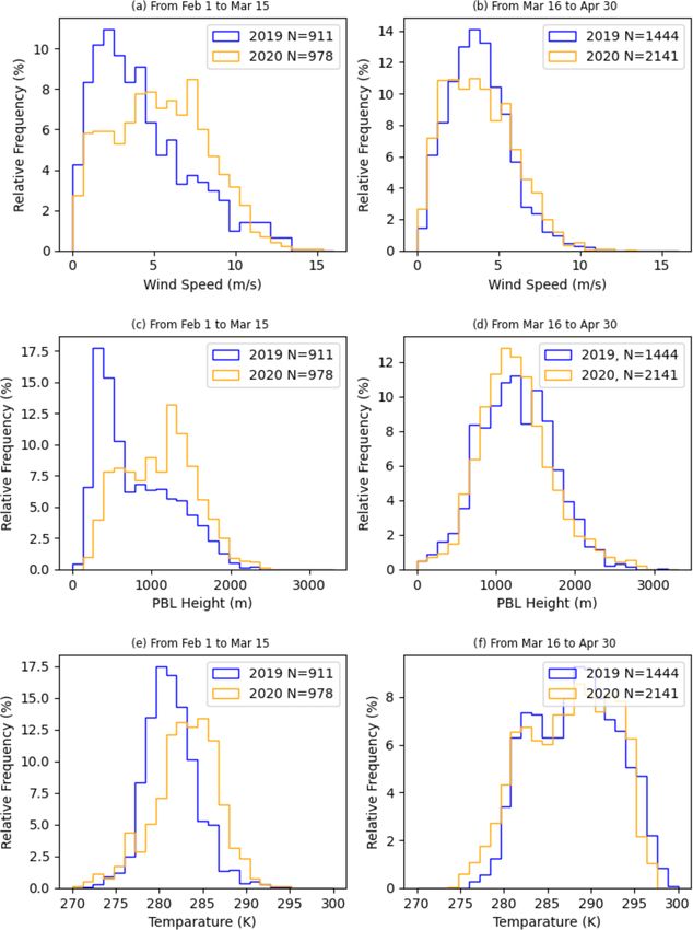
J. Barré et al.: Estimating lockdown-induced European NO2 changes                                                          7375

such analyses place insufficient importance and provide            servations, and air quality models. We firstly illustrate how
insufficient clarity about the fact that satellite data used in    misleading it can be to ignore the influence of the weather
such analyses are conditioned by the cloud coverage, revisit       variability when assessing the lockdown-induced changes
frequency, and quality flag of the satellite observations.         in NO2 with TROPOMI. Then, in order to quantify these
Ignoring or not acknowledging such information can also            changes, we use ML-based weather-normalization methods
lead to flawed satellite-based estimates and provide mislead-      for estimating the “business-as-usual” (BAU) NO2 pollu-
ing information (https://atmosphere.copernicus.eu/flawed-          tion levels that would have been observed without any lock-
estimates-effects-lockdown-measures-air-quality-derived-           down measures, based on both TROPOMI NO2 tropospheric
satellite-observations, last access: January 2021).                columns (Sect. 2) and surface in situ observations (Sect. 3).
   Several studies have investigated lockdown impacts us-          NO2 changes are then investigated with the CAMS regional
ing surface measurement sites. For example, Wang and               ensemble (Sect. 4). We compare and discuss the three differ-
Su (2020) showed that lower emissions from motor vehi-             ent approaches in Sect. 5 followed by conclusions in Sect. 6.
cles and secondary industries were most likely responsible
for the observed decreases in NO2 concentrations in China
during January–March 2020. Collivignarelli et al. (2020)           2     TROPOMI NO2 column estimates
showed using surface station measurements that major NO2
reductions occurred in Milan, a city that showed a rapid           2.1    Dataset and analysis periods
increase in cases early in the European COVID-19 crisis
(February 2020) and was one of the first cities to be put          We use the operational Copernicus S5P TROPOMI NO2
into lockdown in Europe. Past studies such as Carslaw and          level 2 product, for which data have been available since
Taylor (2009) showed the usefulness and the importance of          28 June 2018. These observations are tropospheric columns
weather-normalization techniques for air pollution applica-        (from the surface to the top of the troposphere) with a pixel
tions based on surface observations, such as the local air         resolution of 5.5 km by 3.5 km since 6 August 2019 and 7 km
traffic activity impact on NO2 predictions. This was fol-          by 3.5 km before. The instrument can have an up-to-daily re-
lowed more recently by Grange et al. (2018) and Grange and         visit at 13:30 mean local solar time (LST) assuming clear-
Carslaw (2019), who used machine learning techniques to            sky conditions. The quality flag (qa) provided with the re-
perform weather normalization for analysing trends and de-         trieval is used to select only good-quality data (qa > 0.75),
tecting the impact of policy measures on air quality. Built        which removes cloud-covered scenes, errors, and problem-
on this previous work, several studies made use of machine         atic retrievals (Eskes and Eichmann, 2019). The TROPOMI
learning to estimate the impact of the COVID-19-related mo-        data are then binned on a regular 0.1◦ × 0.1◦ grid to per-
bility restrictions on air pollution levels, taking into account   form statistical analyses and to facilitate the processing of
the confounding effect of the meteorological variability. Us-      time series for the locations of interest, i.e. large European
ing machine learning (ML) models fed with ERA5 reanal-             cities in this study (see Sect. 2.2), as well as the compari-
ysis meteorological data, Petetin et al. (2020) highlighted a      son with other datasets such as the 0.1◦ × 0.1◦ CAMS re-
strong reduction in surface NO2 concentrations across most         gional air quality models (Marécal et al., 2015) and the 9 km
Spanish urban areas during the first weeks of lockdown. Sim-       resolution weather forecasts from the European Centre for
ilarly, Keller et al. (2021) assessed the NO2 pollution changes    Medium-Range Weather Forecasts (ECMWF).
using worldwide surface measurements showing country-                 In this study we consider February, March, and April 2020
dependent variations in reductions.                                and 2019 to assess the changes in NO2 columns due to
   Finally, air quality modelling systems offer a valuable tool    COVID-19 restrictions over Europe. Although the lockdown
for representing the evolution of pollutants in the atmosphere     conditions and dates vary between countries, we consider the
according to changes in emissions, physical processes, and         15 March 2020 to be a representative starting date for the
weather variability. The Copernicus Atmosphere Monitoring          European-wide lockdown given that most European coun-
Service (CAMS) produces daily European air quality fore-           tries implemented their nation-wide social distancing mea-
casts and analyses using an ensemble of 11 models, ensuring        sures along the 2-week period from 9 March 2020 (Italy) to
unique reliability and quality (Marécal et al., 2015). Using       23 March 2020 (United Kingdom, UK). Two periods of the
emission scaling factors to account for lockdown measures,         year are considered in this study: the pre-lockdown period
such an ensemble of models can be used to estimate lock-           from 1 February to 15 March and the lockdown period from
down reductions in NO2 pollution (amongst other pollutants)        16 March to 31 April. This study thus focuses on the most
and account for the weather variability at the same time (Co-      stringent period of the first European lockdown (since many
lette et al., 2020; Guevara et al., 2021).                         countries then started to ease up their lockdown restrictions
   This paper aims to provide a comprehensive and compar-          from the beginning of May onwards).
ative assessment of the impact of the first European COVID-           In Fig. 1, mean TROPOMI NO2 tropospheric columns
19 lockdown on NO2 pollution levels over major European            are displayed for the pre-lockdown and lockdown periods
urban areas using satellite observations, surface in situ ob-      in 2020 and their equivalents in 2019. The comparison of

https://doi.org/10.5194/acp-21-7373-2021                                           Atmos. Chem. Phys., 21, 7373–7394, 2021
7376                                                 J. Barré et al.: Estimating lockdown-induced European NO2 changes

Figure 1. Average maps of the TROPOMI NO2 tropospheric columns (mol m−2 ) for European pre-lockdown and lockdown periods in
2020 (a, b) and corresponding periods in 2019 (c, d). Grey areas indicate where the number of revisits is strictly below five.

pre-lockdown and lockdown averages for 2020 only shows           der colder conditions. These differences in meteorological
a decrease in southern Europe but no clear reduction at          conditions explain the increase in NO2 tropospheric columns
more northern latitudes (i.e. the UK, the Netherlands, and       in 2019 compared to 2020. Conversely, during the post-
Germany). In the corresponding 2019 pre-lockdown period          15 March period, the meteorological distributions are more
much larger NO2 columns are seen than in 2020. During            similar, showing much smaller differences. This illustrates
this period of the year, the meteorological conditions over      the need for accounting for the meteorological effect when
northern Europe were significantly different between 2019        assessing the changes in NO2 tropospheric columns associ-
and 2020. A number of named extratropical cyclones (storms       ated with the lockdown.
Ciara, Denis, Karine, and Myriam), combined with a strong
positive anomaly in surface temperature, occurred over Eu-       2.2   Non-weather-normalized changes in TROPOMI
rope during February and early March 2020, especially in               NO2 tropospheric columns
western and northern Europe. Such anomalies in wind and
temperature were not observed in 2019. Figure 2 shows the
                                                                 Changes in NO2 tropospheric columns associated with the
distribution of 10 m wind speed, planetary boundary layer
                                                                 lockdown measures can be estimated by comparing NO2 lev-
(PBL) height, and 2 m temperature from the 9 km operational
                                                                 els observed during the lockdown period in 2020 with a given
forecasts from the ECMWF Integrated Forecasting System
                                                                 baseline. In this section, we compare the results obtained
(IFS) in both 2019 and 2020 for the pre-lockdown and lock-
                                                                 with two different baselines: (1) the NO2 levels observed dur-
down periods at the S5P overpass times. Details on how
                                                                 ing the pre-lockdown period in 2020 (hereafter referred to as
the PBL height is calculated can be found in the IFS doc-
                                                                 the “before–during” approach), (2) the NO2 levels observed
umentation (part IV, chap. 3 in https://www.ecmwf.int/en/
                                                                 during the same period of the year in 2019 (hereafter referred
elibrary/19748-part-iv-physical-processes, last access: Jan-
                                                                 to as the “year-to-year” approach). We focus our study on
uary 2021). Before 15 March, these parameters show very
                                                                 the largest European urban areas for which the city popula-
different distributions with much lower values in 2019 than
                                                                 tion exceeds 0.5 million inhabitants (according to the pop-
in 2020, i.e. less circulation and less vertical diffusion un-
                                                                 ulation database provided by https://simplemaps.com/data/

Atmos. Chem. Phys., 21, 7373–7394, 2021                                           https://doi.org/10.5194/acp-21-7373-2021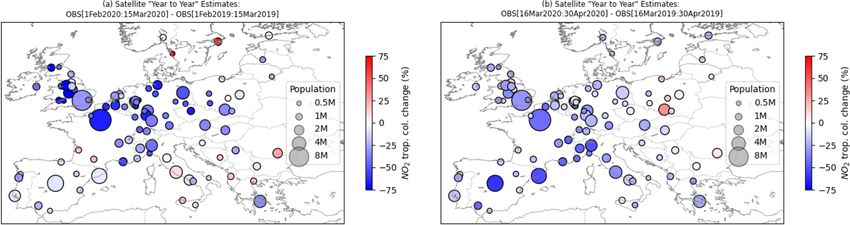
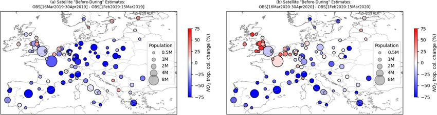
J. Barré et al.: Estimating lockdown-induced European NO2 changes                                                                    7377

Figure 2. Probability density functions of 10 m wind speed (m s−1 ; a, b), planetary boundary layer (PBL) height (m; c, d), and 2 m temper-
ature (K; e, f) from the ECMWF operational forecasts for European periods before (a, c, e) and after 15 March (b, d, f), comparing 2020 to
2019. Distribution is computed for urban areas above 0.5 million inhabitants between 45–60◦ N, 10◦ W–20◦ E, at the S5P overpass times. N
is the sample size for each distribution that can be multiplied by the relative frequency (in %) to obtain the absolute frequency.

world-cities, last access: January 2021), resulting in a total          pre-lockdown and lockdown period. If this condition is not
of 100 locations. Assessing the changes in NO2 tropospheric             met, the location is discarded from the analysis. The before–
columns from satellite observations is more challenging over            during estimate corresponds to the difference between the
rural areas as the NO2 levels are much lower than over urban            pre-lockdown and the lockdown period median estimates.
areas. Because of the much lower NO2 tropospheric-column                Figure 3 shows changes calculated for 2020 (Fig. 3b) and the
values over rural areas, the relative estimates of pollution            equivalent for 2019 (Fig. 3a) for comparison. This method
reduction are very sensitive to small changes in the tropo-             shows drastic NO2 reductions by more than 75 % in 2020
spheric columns and therefore also to instrument noise. We              for most of the large southern European urban areas. Reduc-
choose the observations with footprints closest to the Euro-            tions are, however, not obvious over northern European ur-
pean city centres and with more than five data points per               ban areas and show strong variations from one location to

https://doi.org/10.5194/acp-21-7373-2021                                                  Atmos. Chem. Phys., 21, 7373–7394, 2021
7378                                                  J. Barré et al.: Estimating lockdown-induced European NO2 changes

another. For example, over the UK and Belgium, some ur-           a popular decision-tree-based ensemble method belonging to
ban areas show increases well above 30 %, while other urban       the boosting family. For the predictors, we use the follow-
areas show reductions even though the same lockdown mea-          ing weather and air quality variables from the ECMWF and
sures were applied nationwide. Applying the same method           CAMS operational forecasts at 9 km and 0.1◦ resolutions,
over 2019, a similarly strong decrease in NO2 levels over         respectively: 10 m wind speed and direction, PBL height,
many major European urban areas is visible. Such reductions       2 m temperature, surface relative humidity, geopotential at
in 2019 are not expected in relation to COVID-19 lockdown         500 hPa, and NO2 surface concentrations from the CAMS
measures. Therefore, such a before–during type of satellite-      regional ensemble forecasts. The NO2 surface concentrations
based estimates does not provide a robust methodology for         used here are obtained from the CAMS operational regional
assessing the effects of the COVID-19 lockdown on Euro-           forecasts, which are based on business-as-usual emission in-
pean NO2 pollution levels.                                        formation and are therefore different from the simulations
   The year-to-year approach has been more widely used in         presented in Sect. 4. In the CAMS regional forecast product,
scientific publications and web news articles and consists        there is also no assimilation of observations to constrain the
of comparing observations from 2020 to observations from          forecasts. Therefore, the NO2 surface concentrations used to
2019 over the period of interest. Figure 4 shows such year-to-    train and make model predictions do not include lockdown
year estimates, comparing the median values between 2020          effects and are independent of the air quality model pollution
and 2019, for the pre-lockdown (Fig. 4a) and lockdown             change estimates provided in Sect. 4. Additionally, the fol-
(Fig. 4b) periods. During the lockdown, an overall reduc-         lowing time and location variables were also included in the
tion is seen all over Europe, with more moderate reductions       set of predictors: latitude, longitude, population, Julian date
over southern Europe compared to the before–during esti-          (number of days since 1 January), and weekday (to reflect
mates (see Fig. 3b). Changes over northern Europe do not          expected weekend and weekday effects). Quite similar ML-
show strong variations between the various urban areas, as        based approaches have already been successfully applied to
was visible in the before–during method. An overall decrease      in situ surface air quality (AQ) observations (e.g. Grange et
is seen over most European locations, with the strongest re-      al., 2018; Grange and Carslaw, 2019; Petetin et al., 2020).
ductions in European countries (e.g. France, Spain, or Italy),    We use data from 1 January to 31 May 2019 as a training
where lockdown measures were more stringent (according to         set and apply the model to 2020 to generate simulations of
the Oxford Coronavirus Government Response Tracker strin-         BAU NO2 tropospheric columns. For validation purposes,
gency index; Hale et al., 2021). However, looking at the pre-     we have randomly split the input data in a 90 % and 10 %
lockdown estimates, northern Europe also shows drastic neg-       share for training and testing, respectively. Hyperparameter
ative changes that are larger than during the lockdown period.    tuning (see Appendix A for details) was performed using a
Such changes in pollution levels across Europe should not be      grid search method with fivefold cross-validation and using
expected if only the impact of emission changes was con-          the ranges indicated by Petetin et al. (2020). In contrast to
sidered. The year-to-year method thus appears to be strongly      Petetin et al. (2020), who trained one ML model per surface
dependent on the interannual NO2 variability, where meteo-        air quality monitoring station, only one single ML model is
rology plays a crucial role. Although it respects the seasonal-   trained here for all cities. This choice is motivated by the
ity of NO2 , this method could still lead to large errors when    small size of the available training dataset (about 10 000 data
assessing differences in NO2 levels and more generally the        points; see Table 1). After the hyperparameter tuning and
pollution level reductions due to the COVID-19 lockdown.          evaluation of the model, the BAU observation simulations
                                                                  have been generated using 100 % of the January–May 2019
2.3     Weather-normalized changes in TROPOMI NO2                 dataset to use the maximum number of data points possible.
        tropospheric columns
                                                                  2.3.2   Results
2.3.1    Methods
                                                                  Detailed scores of the performance of the gradient boosting
Weather-normalization methods account for weather vari-           regressor with respect to TROPOMI observations, such as
ability to more accurately estimate the net changes in NO2        mean bias (MB), normalized mean bias (nMB), root mean
induced by the lockdown in urban areas. Previous studies          square error (RMSE), normalized root mean square error
have used meteorological and air pollution predictors to build    (nRMSE), and the Pearson correlation coefficient (PCC), can
simplified models for the simulation of satellite observations    be found in Table 1. In order to check for obvious cases
or to generate predictions of atmospheric composition (e.g.       of overfitting (i.e. when the GBM model is fitting the data
Worden et al., 2013; Barré et al., 2015). In this study, we       used for training too closely and is thus lacking generaliza-
use a novel approach for the simulation of TROPOMI satel-         tion skills regarding new data), results are shown for both
lite observations under BAU conditions, i.e. in the absence       training and testing datasets. The statistics for the training
of lockdown restrictions, based on the gradient boosting ma-      set and the testing set show similar results, such as low bias,
chine (GBM; Friedman, 2001) regressor technique. GBM is           good correlation, and significant RMSE values. The statisti-

Atmos. Chem. Phys., 21, 7373–7394, 2021                                             https://doi.org/10.5194/acp-21-7373-2021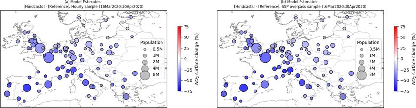
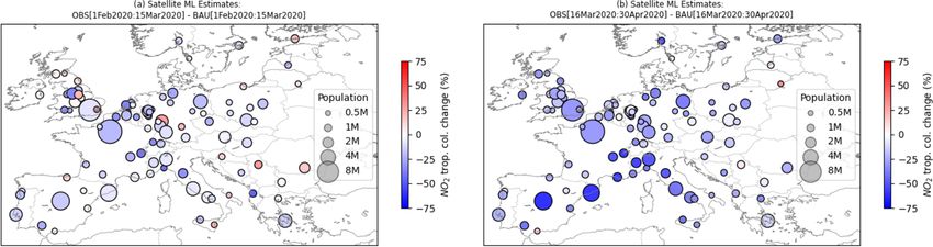
J. Barré et al.: Estimating lockdown-induced European NO2 changes                                                            7379

Figure 3. Before–during estimates of TROPOMI tropospheric NO2 column change (%) for urban areas above 0.5 million inhabitants in
2019 (a) and 2020 (b). The diameter of the circles is proportional to the population count in each urban area.

Figure 4. Year-to-year estimates of TROPOMI tropospheric NO2 column change (%) for urban areas above 0.5 million inhabitants in
2019 (a) and 2020 (b). The diameter of the circles is proportional to the population count in each urban area.

cal performance obtained for the training set indicates that         vations. This shows that the GBM predictions based on BAU
there is no clear sign of overfitting in the predictions. Since      predictors perform realistically and account for the variabil-
TROPOMI data are only available from mid-2018 onwards,               ity in the BAU scenario. This therefore provides a method
the training set is relatively small. For this reason, the predic-   to assess the pollution changes due to lockdown restrictions
tions are featuring significant RMSE values and will have a          using satellite data more robustly than the before–during or
large random error. The RMSE values stay, however, within            year-to-year methods.
a similar range as for the surface site air quality ML pre-             Figure 6 shows the equivalent estimates as in Figs. 3 and
dictions, as shown in Sect. 3 and Table 2. The low mean              4 for the pre-lockdown and lockdown periods using the ML-
bias and high correlation values indicate that the main BAU          based BAU estimates as the baseline. The estimates of the
NO2 tropospheric-column variability is represented without           NO2 changes are based on the median value of the real obser-
large systematic errors. Subtracting the simulated BAU NO2           vation minus the simulated BAU observation distributions.
columns from the actual observed NO2 columns during the              As shown in Table 1, the GBM performance shows large
lockdown period (from 16 March to 30 April 2020) gives us            RMSE values, which can sometimes result in significant out-
an estimate of the reductions in the NO2 background levels           liers due to the small training set used. We choose to dis-
over the urban areas considered in this study. Figure 5 pro-         play the median to avoid the influence of potential outliers
vides an example of a time series over Madrid that shows the         in the estimates as much as possible. The pre-lockdown ML-
behaviour of the GBM against the real observations for 2019          based estimates do not show as strong of an overall reduc-
(the training period) and 2020 (the actual simulation period).       tion as in the year-to-year (Fig. 4) or before–during (Fig. 3)
In 2019, the GBM predictions follow the variations seen in           estimates. A summary of the average and the standard de-
the observations but do, however, also show differences, be-         viation of the set of median estimates across all the consid-
ing either above or below the observations. In 2020, simi-           ered European urban areas is provided in Table 2 for each
lar behaviour is observed until the lockdown date, when the          of the satellite methods. While both year-to-year and before–
GBM predictions show consistently higher values than the             during methods showed substantial changes (24 % and 30 %,
observations but still follow the same variations as the obser-      respectively) in NO2 during the periods outside lockdown

https://doi.org/10.5194/acp-21-7373-2021                                             Atmos. Chem. Phys., 21, 7373–7394, 2021
7380                                                     J. Barré et al.: Estimating lockdown-induced European NO2 changes

Table 1. Performance of the machine learning simulations of NO2 tropospheric columns over all European urban areas included in the
dataset. The training set and testing set cover January–May 2019 and are randomly sampled (90 % and 10 %, respectively) over that period.
Shown are the mean bias (MB), normalized mean bias (nMB), root mean square error (RMSE), normalized root mean square error (nRMSE),
Pearson correlation coefficient (PCC), and the number of data points (N).

                                                     MB       nMB             RMSE       nRMSE      PCC        N
                                          (10−6 mol m−2 )      (%)    (10−6 mol m−2 )       (%)
                       S5P training set             0.00     +0.02                 1.4      45.68    0.87   9634
                       S5P test set                −0.04     −1.30                1.68      56.38    0.79   1071

Figure 5. Example of a time series over Madrid illustrating the performance of the machine learning NO2 column predictions for February–
March–April 2019 (a) and the same period in 2020 (b).

Atmos. Chem. Phys., 21, 7373–7394, 2021                                                  https://doi.org/10.5194/acp-21-7373-2021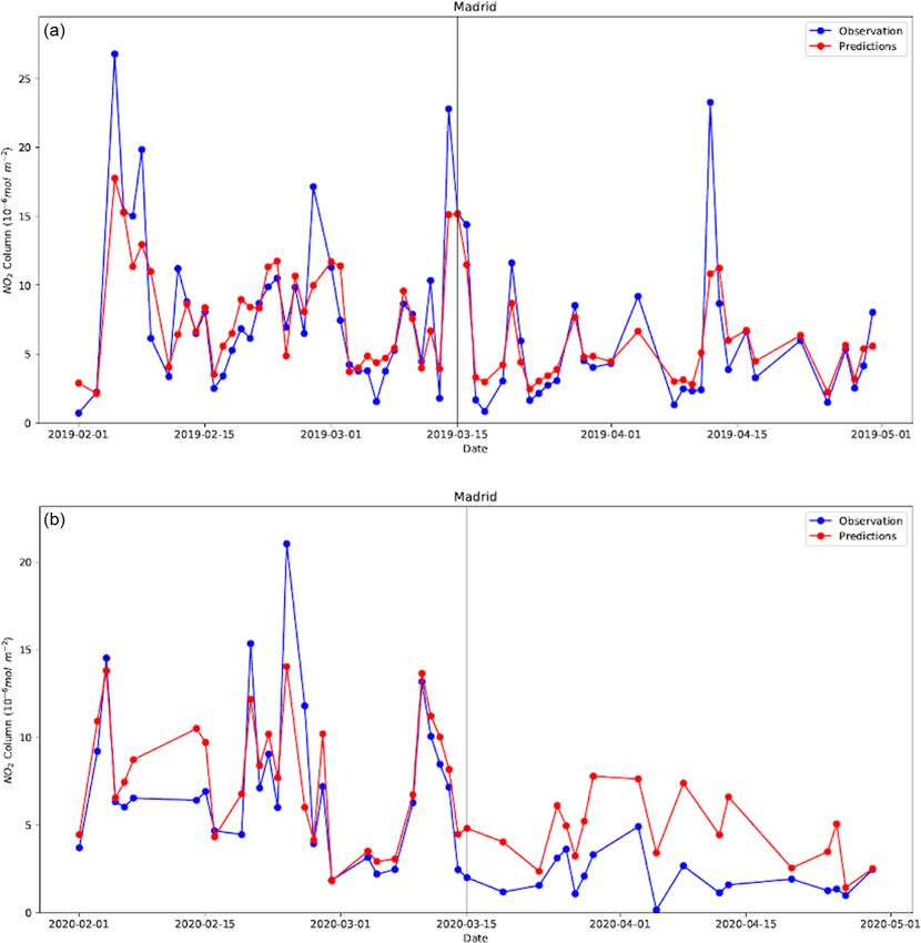
J. Barré et al.: Estimating lockdown-induced European NO2 changes                                                                7381

Figure 6. TROPOMI-based estimation of tropospheric NO2 column change (%; relative to the BAU predictions) for urban areas with at least
0.5 million inhabitants, computed using the ML-based weather-normalization method for the pre-lockdown and lockdown periods (a and b,
respectively). The diameter of the circles is proportional to the population count in each urban area.

Table 2. Scores over all European urban areas included in the           riod, and on average, across Europe, the year-to-year and
dataset for the different TROPOMI NO2 tropospheric-column-              weather-normalized estimates show results within the same
change estimates. Mean and standard deviation are calculated for        range in terms of mean (around −20 %) and variability
the median estimates of all urban areas considered in the study; i.e.   amongst the median estimates obtained for all urban areas
the standard deviation is a metric of the inter-urban-area spread.      (around 16 %). This is, however, not the case for the before–
Dates are in dd/mm.
                                                                        during estimates, which show much stronger variability be-
                                            Mean      Standard
                                                                        tween European urban areas (62 %). The before–during esti-
                                             (%)     Deviation          mates are therefore not reliable, and the year-to-year method
                                                           (%)          is very dependent on the differences in the meteorological
                                                                        situations between 2019 and 2020. For this reason, the ML
     Before–during (2019)                    −40            47          estimates are the most reliable and will be used solely for
     Before–during (2020)                    −25            62
                                                                        the rest of this study. Details of the ML estimates during the
     Year-to-year (01/02 to 15/03)           −26            31
                                                                        lockdown provided in Fig. 6 are reported in the Table B1
     Year-to-year (16/03 to 30/04)           −18            16
     Machine learning (01/02 to 15/03)        −8            16          in Appendix B. The NO2 tropospheric-column-change es-
     Machine learning (16/03 to 30/04)       −23            16          timates (median values per urban area) show on average a
                                                                        reduction of 23 %, but urban areas that are known to have
                                                                        the most stringent measures (Hale et al., 2021) show much
                                                                        stronger reductions, e.g. Madrid (60 %), Barcelona (59 %),
(i.e. in 2019 or before the lockdown in 2020) when low to               Turin (54 %), and Milan (49 %). Lighter reductions can be
no reduction should be expected, the ML-based weather-                  observed in urban areas where less stringent measures were
normalization method provides changes closer to 0 %, which              taken, e.g. Stockholm (17 %). To check the robustness of
are considered to be more realistic.                                    these results, equivalent estimates are provided using surface
   The weather-normalization method is not devoid of uncer-             stations and air quality models in Sects. 3 and 4 and will be
tainties and can, in particular, be affected by trends in NO2           compared in Sect. 5.
levels. With a known trend seen in European NOx emissions
of around 2 % yr−1 to 4 % yr−1 (EEA, 2020a) and only 1                  3     Surface station estimates
year to train the data, the ML method potentially provides a
stronger-than-expected overall reduction of around 8 %. The             3.1    Methods
before–during and the year-to-year approaches also show
stronger reduction estimates on average during 2019 and the             We have estimated the impact of the COVID-19 lock-
pre-lockdown period, respectively. The latter two methods               down on surface NO2 pollution in European areas using the
also display a stronger standard deviation across cities than           methodology introduced by Petetin et al. (2020), applied to
the weather-normalization method, which suggests substan-               up-to-date (i.e. partly non-validated real-time) hourly NO2
tial local biases due to the omission of the meteorological             data from the EEA AQ e-reporting (https://www.eea.europa.
variability.                                                            eu/data-and-maps/data/aqereporting-8, last access: January
   When we consider the lockdown period, the weather pa-                2021). We first selected the urban and suburban background
rameter distributions are much more similar between 2019                stations located within 0.1◦ from the city centres and ap-
and 2020 (Fig. 2) than is the case for the pre-lockdown pe-             plied the quality assurance and data availability screening

https://doi.org/10.5194/acp-21-7373-2021                                                 Atmos. Chem. Phys., 21, 7373–7394, 2021
7382 J. Barré et al.: Estimating lockdown-induced European NO2 changes
described in Petetin et al. (2020), using the GHOST (Glob- to the fact that we are working with hourly estimates here.
ally Harmonised Observational Surface Treatment) metadata This is demonstrated by similar results as those of Petetin et
(Bowdalo et al., 2021). A total of 164 stations in 77 urban al. (2020) that are obtained over this set of European cities
areas was selected. At each station (independently), we es- when predicting NO2 at the daily scale (for the test dataset:
timated the BAU NO2 mixing ratios that would have been nRMSE = 28 %, PCC = 0.88, N = 11 082).
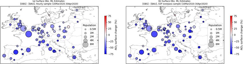
observed during the lockdown period under an unchanged For a stricter comparison with the results discussed in
emission forcing. This was done using GBM models fed with Sect. 2, we provide two different estimates to assess the satel-
meteorological inputs (2 m temperature, minimum and maxi- lite sampling effect: (i) using all hourly values or (ii) filtered
mum 2 m temperature, surface wind speed, normalized 10 m according to the S5P satellite overpass time (13:30 LST) and
zonal and meridian wind speed components, surface pres- “qa” filtering (clear sky only). Figure 7 displays relative
sure, total cloud cover, surface net solar radiation, surface change estimates, showing the median of the distributions for
solar radiation downwards, downward UV radiation at the each European city above 0.5 million inhabitants. Overall,
surface, and PBL height) taken from the 31 km horizontal the estimates for both sampling strategies are broadly con-
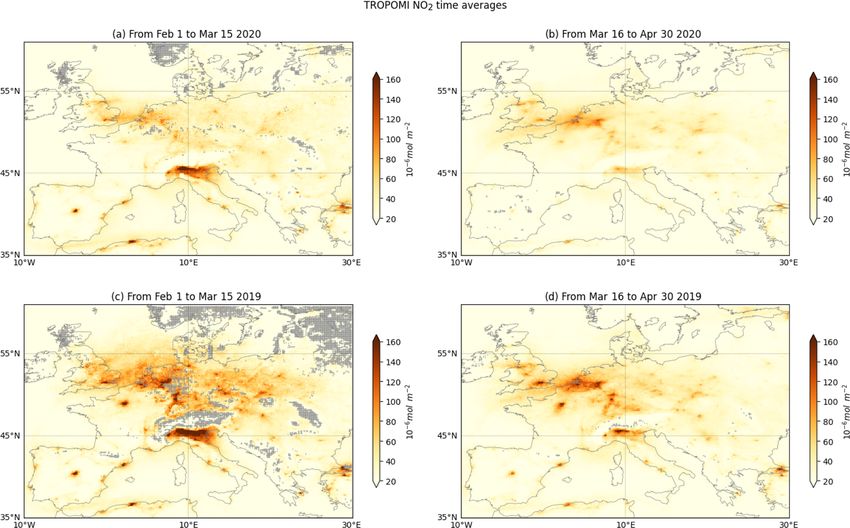
resolution ERA5 reanalysis dataset (Hersbach et al., 2020) in sistent, with NO2 reductions of around 37 % and 43 % on
addition to other time features (date index, Julian date, week- average for the hourly sampling and the S5P overpass sam-
day, hour of the day). The ERA5 reanalysis dataset is a con- pling, respectively (Table 3). The surface station estimates
sistent model version over time but at coarser resolution in also show geographical variations similar to the satellite esti-
comparison to the ECMWF high-resolution operational fore- mates, with larger reductions corresponding to locations with
casts used in the TROPOMI estimates (31 km versus 9 km). more stringent lockdowns (i.e. Spain, Italy, and France) and
All GBM models were trained and tuned with data for the less stringent lockdowns (i.e. Sweden, Germany). For exam-
past 3 years (2017–2019) and tested with data from 2020 be- ple, Madrid shows reductions of 61 % and 60 % using the
fore the lockdown. Petetin et al. (2020) showed that such du- hourly surface stations and the satellite overpass time sam-
ration for training the GBM models is generally sufficient for pled surface stations, which are very similar to the satellite
capturing the influence of the weather variability on surface estimates. In contrast, Stockholm shows very small reduc-
NO2 mixing ratios. As discussed in more detail in Petetin et tions of 8 % and 3 %, respectively. These latter values are dif-
al. (2020), the date index feature here allows the limitation ferent from the satellite-based estimates (reduction of 17 %)
of the potential issues related to the presence of trends in the and point out some uncertainty regarding the estimates in this
NO2 time series (between a 2 % and 4 % decrease per year; area.
EEA 2020a). If a substantial trend exists, the GBM models Northern Europe (particularly Germany, Poland, and the
will put more importance on this feature, which in practice UK) displays larger NO2 reductions with the estimates at
will force the model to make NO2 mixing ratio predictions satellite overpass time. This points out a possible dependence
(in 2020) in the range of the values observed during the last on the time of the day in the emission and pollution reduc-
part of the training dataset, ignoring the oldest training data. tions. In general, those relative NO2 changes based on the
Thus, given the long-term reduction in NO2 resulting from surface in situ observations are larger than the ones based
policy measures across Europe, considering longer training on satellite NO2 tropospheric columns. These two points are
periods is not expected to improve the performance of the further discussed in Sect. 5.
GBM models. In contrast to Petetin et al. (2020), who pre-
dicted BAU NO2 at a daily scale, the ML models developed
here are predicting NO2 at an hourly scale (in order to get 4 CAMS regional ensemble model estimates
results collocated in time with TROPOMI overpasses; see
4.1 Methods
also below). We then deduced the weather-normalized NO2
changes due to the lockdown by comparing observed and Model estimates have been calculated using the CAMS Eu-
ML-based BAU NO2 mixing ratios. ropean regional air quality forecasting framework, which is
an ensemble of 11 models (Marécal et al., 2015). These
3.2 Results models are used to calculate multi-model median values,
which are the best-performing quantity on average com-
Table 3 shows the overall performance of the GBM models pared to individual models. Using such a multi-model ap-
in the training and test data sets. Statistical results are similar proach is useful to minimize the imperfections in each
to the TROPOMI NO2 GBM model. Biases are low, correla- model formulation. Operational evaluation and validation
tion is high, and there is a significant RMSE. As explained in of the CAMS European ensemble against independent ob-
Sect. 2.3.2, statistical scores in the training set and the test servations are performed and delivered routinely and can
set suggest that there is no apparent sign of overfitting in be accessed at https://atmosphere.copernicus.eu/index.php/
the predictions showing reasonable performance. Note that regional-services (last access: January 2021).
the RMSE and PCC are deteriorated compared to the statis-
tics obtained over Spain in Petetin et al. (2020), mainly due
Atmos. Chem. Phys., 21, 7373–7394, 2021 https://doi.org/10.5194/acp-21-7373-2021J. Barré et al.: Estimating lockdown-induced European NO2 changes 7383
Figure 7. Weather-normalized estimation of NO2 changes (%; relative to the BAU predictions) using surface observations during the lock-
down period using business-as-usual (BAU) simulated observations as the baseline for urban areas with at least 0.5 million inhabitants.
Panel (a) shows the estimates using full hourly datasets, and panel (b) shows the estimates using the S5P-sampled overpass time dataset. The
diameter of the circles is proportional to the population in each urban area.
Table 3. Performance of the ML predictions of hourly NO2 surface mixing ratios over all European urban areas included in the dataset.
MB nMB RMSE nRMSE PCC N
(ppbv) (%) (ppbv) (%)
Surface station training set (2017–2019) 0.0 0.0 5.53 40.88 0.84 4 048 696
Surface station test set (1 Jan–15 Mar 2020) +0.95 +7.02 6.24 45.87 0.80 268 960
Two sets of model hindcasts have been conducted using bility Reports (https://www.google.com/covid19/mobility/,
two different emission scenarios: BAU emissions and re- last access: January 2021) for road transport, airport statis-
duced COVID-19 lockdown emissions. The emission inven- tics from Flightradar24 (https://www.flightradar24.com/data/
tory used for the BAU reference simulation is the same that is airports, last access: January 2021) for aviation, and electric-
used in the daily regional air quality forecasts of CAMS for ity load information from the European Network of Trans-
Europe, i.e. the CAMS-REG-AP dataset (v3.1 for the refer- mission System Operators for Electricity (ENTSO-E; https:
ence year 2016; Granier et al., 2019). It is compiled by TNO //transparency.entsoe.eu/, last access: January 2021) for the
(Netherlands Organisation for Applied Scientific Research) industry sector. Results from Guevara et al. (2021) showed
under the CAMS emission service, based on official emis- that during the most severe lockdown period (23 March to
sions reported by the countries to the EU (National Emis- 26 April), estimated surface emission reductions at the Eu-
sions reduction Commitments (NEC) Directive) and United ropean level were most important for NOx (33 %), with road
Nations Economic Commission for Europe (UNECE; Long- transport being the main contributor to total reductions in all
range Transboundary Air Pollution (LRTAP) Convention– cases (85 % or more). Italy, France, and Spain were the coun-
European Monitoring and Evaluation Programme (EMEP); tries that experienced major NOx emission reductions (down
Kuenen et al., 2014). The spatial resolution of the emissions to 50 %), a result that is in line with the strong lockdown re-
is 0.1◦ × 0.05◦ but re-gridded to 0.1◦ × 0.1◦ to match the strictions implemented by their respective governments. In
models’ grid. The alternative emission scenario, correspond- contrast, Sweden, for example, showed reductions of only
ing to the lockdown period, was derived by combining the 15 % (on NOx ) due to the implementation of national rec-
original CAMS-REG-AP inventory with a set of country- and ommendations instead of a state-enforced lockdown. More
sector-resolved reduction factors (Guevara et al., 2021). For details about the emission scaling procedure using the data
the present work, time-invariant emission reduction factors and methodology from Guevara et al. (2021) can be found
were used by country and for three activity sectors: manu- in Colette et al. (2020), where the resulting country and ac-
facturing industry, road transport, and aviation (landing and tivity sector-dependent reduction factors are provided for the
take-off cycles), which are reduced on average by 15.5 %, EU28 countries plus Norway and Switzerland. Values of the
54 %, and 94 %, respectively. These sectors were considered emission reduction factors per country within the European
to be the most affected by changes in activity during lock- regional modelling domain and per activity sector are pro-
down (Le Quéré et al., 2020). vided in Appendix C. For the main contributing sector, road
The reduction factors were computed from collections of transport, the largest reductions in emissions are observed in
near-real-time activity data, such as Google Community Mo- countries where lockdown restrictions were more stringent
https://doi.org/10.5194/acp-21-7373-2021 Atmos. Chem. Phys., 21, 7373–7394, 20217384 J. Barré et al.: Estimating lockdown-induced European NO2 changes
(according to the Oxford Coronavirus Government Response Table 4. Scores over all European urban areas included in the study
Tracker stringency index; Hale et al., 2021), such as Italy for the different NO2 change estimates: based on surface obser-
(75 %), Spain (80 %), and France (76 %). vations, model estimates, and TROPOMI observations. Mean and
All the models operated with the same set-up as the CAMS standard deviation are calculated for all resulting urban-area esti-
regional operational production. The modelling domain cov- mates; i.e. the standard deviation is a metric of the inter-urban-area
spread.
ers Europe at 0.1◦ × 0.1◦ resolution. The meteorological and
chemical boundary conditions are obtained from the Inte-
Mean Standard
grated Forecasting System (IFS) of the ECMWF, which is
(%) deviation
the same system that provides part of the dataset for the (%)
ML-based estimations (see Sects. 2 and 3). The baseline
simulation was using the BAU anthropogenic emissions as Surface stations (hourly) −37 15
described above, and the lockdown scenario was using the Surface stations (S5P sampling) −43 19
lockdown-adjusted inventory, modulated by country and ac- CAMS model ensemble (hourly) −30 11
CAMS model ensemble (S5P sampling) −32 12
tivity sectors. From the two sets of 11 model simulations,
TROPOMI −23 16
the median at each grid point is calculated from an ensemble
simulation (as is routinely done for the operational CAMS
predictions; Marécal et al., 2015). Differences between the
BAU ensemble and the lockdown scenario ensemble are then lion inhabitants. The values of each estimate for all urban
used to calculate NO2 reduction estimates. areas considered in this study are given in Table B1 in Ap-
pendix B.
4.2 Results The three types of weather-normalized estimates agree
on identifying stronger reductions where more severe lock-
Figure 8 displays the relative change estimates for each Eu- down measures were implemented. As shown in Sect. 2,
ropean urban area defined in Sect. 2.2. The estimates are satellite-based estimates show a relationship between NO2
calculated using the median of the full hourly distribution tropospheric-column reductions and the extent and gener-
(Fig. 8a) and of the distribution at qa-filtered S5P overpass alization of restrictive measures in each country. A simi-
times and dates only (Fig. 8b) for each urban area. As ex- lar relationship is observed for surface sites and model es-
pected, urban areas in more stringent lockdown countries (i.e. timates (Sects. 3 and 4). The largest NO2 reduction estimates
Spain, Italy, France) show the largest reductions (e.g. down of around 50 % to 60 % for both surface and tropospheric
to 60 % in Madrid; see Fig. 9), whereas urban areas with less columns are found in Spanish, Italian, and French urban
stringent lockdown measures (i.e. Germany, Poland, Swe- areas. In countries that implemented softer lockdown mea-
den) show smaller reductions (e.g. around 16 % in Stock- sures, urban areas show smaller reductions, e.g. Germany,
holm; see Fig. 8). The time sampling difference (hourly ver- Netherlands, Poland, and Sweden. Although significant dis-
sus S5P overpass) does not affect the model estimates much; crepancies exist between the satellite-, surface-, and model-
only differences of a few per cent are seen for most of the based estimates in urban areas such as Naples (Italy), Sofia
European urban areas. On average, over the set of median (Bulgaria), and Katowice (Poland), the three methods pro-
estimates for each urban area, the difference is small, with vide an overall consistent picture. It is remarkable to note
30 % for hourly estimates and 32 % for S5P-sampled esti- that this result contributes to establishing the usefulness of
mates. This is expected as the emission reduction estimates satellite-based estimates for urban air quality and not only
used to generate the lockdown scenario ensemble are set con- for atmospheric pollution in general. Having a range of three
stant over time (daily and hourly). This point is further ex- different types of estimates helps to provide estimates of pol-
panded in the next section, where model estimate results are lution changes across Europe with a certain level of certainty.
compared to the other types of estimates. When all the estimates agree, it is more likely that the values
of reduction due to the lockdown implementations are reli-
able. Conversely, if the different types of estimates show dis-
5 Comparison of the three different types of estimates crepancies, less confidence should be given to the reduction
estimates. In Fig. 8, Madrid, Turin, and Milan, to mention
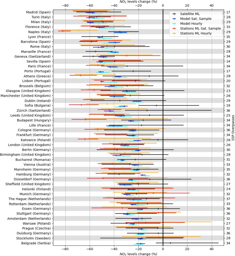
In Table 4 and Fig. 9 we summarize the results of this study. a few urban areas, show consistency between the different
Table 4 shows the average reduction in all the median esti- types of estimates, expressing more certainty in the results.
mates together with the inter-urban-area variability over Eu- In other locations such as Sofia, Athens, and Budapest, strong
rope. Figure 9 shows the distribution of the NO2 changes discrepancies indicate that the estimates could be uncertain.
estimated for the lockdown period per urban area. This fig- Average scores in Table 4 show that surface station observa-
ure provides estimates equivalent to box plots where the me- tions provide stronger reduction estimates and that satellite-
dian and the interquartile range are displayed. For clarity, we based estimates provide weaker reduction estimates. Model
chose to display only urban areas that have more than 1 mil- estimates are mostly in between and show much less spread
Atmos. Chem. Phys., 21, 7373–7394, 2021 https://doi.org/10.5194/acp-21-7373-2021J. Barré et al.: Estimating lockdown-induced European NO2 changes 7385 Figure 8. Air quality modelling estimates of surface NO2 changes (%; relative to the BAU predictions) during the lockdown period in urban areas with at least 0.5 million inhabitants. Panel (a) shows the estimates using full hourly datasets, and panel (b) shows the estimates using the S5P-sampled overpass time dataset. The diameter of the circles is proportional to the population in each urban area. within a given urban area (bars in Fig. 9) and less variation age is the information given by the models or the satellites. between urban areas (standard deviation in Table 4). The ori- These representativeness issues contribute to creating dis- gin of such differences can vary and is detailed below. crepancies between the type of estimates and hence generate Machine learning estimates that are observation-based uncertainty. The differences seen in Fig. 9 between surface (satellite and surface stations) show more spread compared station estimates and gridded estimates (models and satel- to the model estimates. In Fig. 9 the interquartile ranges for lites) point out such possible representativeness issues. Rep- the observation-based ML estimates are much larger than for resentativeness is a difficult and important topic and deserves the model estimates. Such large ranges show that there is further research as it would require careful examination of a strong spread in the ML-based estimates that is not seen the stations’ locations in specific urban areas and also using in the model-based estimates. Model estimates are based higher-resolution modelling than 10 km. on country-dependent emission reduction or scaling factors Satellite overpass times (13:30 LST) and the presence of that are constant over time. The variability is induced by the clouds in the measurement pixel can potentially influence changes in atmospheric conditions but not by changes in the the reduction estimates from the TROPOMI data. We con- emissions. The estimates from the ML approach can repre- sidered 1.5 months to compute the satellite reduction esti- sent the transition into the lockdown where emissions gradu- mates. Overall, the sample size (valid S5P overpasses) in ally decreased. This contributes to the increased spread seen Fig. 9 ranges between 14 (Sevilla) and 37 (The Hague). Also in the ML estimates. Scores from ML estimates (see Tables 1 in Fig. 9, surface sites and model estimates are displayed for and 3) also show significant RMSE that can add noise to the hourly and S5P-sampled estimates. Smaller or larger samples time series and add to the resulting spread of the distribu- cannot really explain discrepancies between all the different tions. A stronger spread in TROPOMI estimates is likely due estimates. Results, however, can be affected when the sam- to the small training set used. Disentangling the noise and ple size becomes statistically very small and if shorter time the actual variability would need to be done carefully in fu- periods (e.g. 1 or 2 weeks) are considered for satellite reduc- ture work. tion estimates. Very small samples over the 6-week period All the different estimates presented in this study are con- were not considered in this study to avoid this effect. The sistent in their spatial scale, using 0.1◦ × 0.1◦ TROPOMI- sampling effect also shows greater changes in the surface averaged pixels that match the CAMS forecasts and surface station estimates than in the model estimates. As mentioned stations within a 0.1◦ range from the city centre. Some of above and seen in Fig. 9, the surface station estimates pro- the smaller urban areas considered in this study likely have a vide more variability that accounts for hourly variations. The footprint that is smaller than 0.1◦ , meaning that high pollu- model estimates have fixed emission scaling factors for the tion levels from the urban area are mixed with low pollution entire lockdown period. The surface station estimates show background levels. This could cause the pollution changes more sensitivity to the time sampling than the model esti- in the gridded estimates to be weaker than expected in cer- mates. On average (see Table 4), the S5P overpass sampling tain urban areas (e.g. Katowice, Budapest, Glasgow, etc.). changes the estimates by around −6 % for surface station es- Also, even if the urban and suburban background stations timates and only by −1.5 % for model estimates. This sug- are selected, the in situ surface observations sample the pol- gests that the lockdown-induced reduction estimates depend lution levels within a 0.1◦ × 0.1◦ pixel given their location. upon the time of the day, i.e. those times when the road trans- This sampling might not be exactly representative of the av- port activity peaks. erage pollution footprint within the same pixel. This aver- https://doi.org/10.5194/acp-21-7373-2021 Atmos. Chem. Phys., 21, 7373–7394, 2021
7386                                                       J. Barré et al.: Estimating lockdown-induced European NO2 changes

Figure 9. Comparisons of the lockdown-induced NO2 change estimates (%; relative to the BAU predictions) using different methodologies
for European urban areas above 1 million inhabitants. Horizontal lines represent the interquartile ranges (over the temporal variability), and
the ticks are the median values using the full distribution per urban area. For readability, urban areas are ranked using the average between
all median estimates.

   Finally, the reduction estimates for tropospheric NO2                 sidered, the satellite estimates show around 23 % reduction
columns displayed in Fig. 9 are generally not as strong as               on average, which is 10 % to 20 % less than the model and
the NO2 surface estimates (observations and model). Some                 surface station estimates (see Table 4). This can be expected
exceptions can be seen in certain Spanish (e.g. Barcelona,               as NO2 surface site measurements do not directly translate
Madrid) and Italian (e.g. Milan, Turin) urban areas, where               to the TROPOMI NO2 tropospheric column, which is the in-
column estimates are close to the surface estimates, but over-           tegrated NO2 content from the surface to about 200 hPa alti-
all column reductions are weaker. With all urban areas con-              tude. Due to the short lifetime of NO2 (around 12 h), only

Atmos. Chem. Phys., 21, 7373–7394, 2021                                                     https://doi.org/10.5194/acp-21-7373-2021
You can also read