Quality assessment for site characterization at seismic stations
←
→
Page content transcription
If your browser does not render page correctly, please read the page content below
Bulletin of Earthquake Engineering
https://doi.org/10.1007/s10518-021-01137-6

    ORIGINAL ARTICLE

Quality assessment for site characterization at seismic
stations

Giuseppe Di Giulio1           · Giovanna Cultrera2         · Cécile Cornou3   · Pierre‑Yves Bard3       ·
Bilal Al Tfaily3

Received: 12 November 2020 / Accepted: 25 May 2021
© The Author(s) 2021

Abstract
Many applications related to ground-motion studies and engineering seismology benefit
from the opportunity to easily download large dataset of earthquake recordings with differ-
ent magnitudes. In such applications, it is important to have a reliable seismic characteriza-
tion of the stations to introduce appropriate correction factors for including site amplifica-
tion. Generally, seismic networks in Europe describe the site properties of a station through
geophysical or geological reports, but often ad-hoc field surveys are missing and the char-
acterization is done using indirect proxy. It is then necessary to evaluate the quality of a
seismic characterization, accounting for the available site information, the measurements
procedure and the reliability of the applied methods to obtain the site parameters.In this
paper, we propose a strategy to evaluate the quality of site characterization, to be included
in the station metadata. The idea is that a station with a good site characterization should
have a larger ranking with respect to one with poor or incomplete information. The pro-
posed quality metric includes the computation of three indices, which take into account
the reliability of the available site indicators, their number and importance, together with
their consistency defined through scatter plots for each single pair of indicators. For this
purpose, we consider the seven indicators identified as most relevant in a companion paper
(Cultrera et al. 2021): fundamental resonance frequency, shear-wave velocity profile, time-
averaged shear-wave velocity over the first 30 m, depth of both seismological and engineer-
ing bedrock, surface geology and soil class.

Keywords Seismic characterization · Quality metrics · Site survey · Seismic station
metadata · Seismic network database · Strong-motion database

* Giuseppe Di Giulio
  giuseppe.digiulio@ingv.it
1
      Istituto Nazionale di Geofisica e Vulcanologia, L’Aquila, Italy
2
      Istituto Nazionale di Geofisica e Vulcanologia, Rome, Italy
3
      Universitè Grenoble Alpes, Universitè Savoie Mont Blanc, CNRS, IRD, Université Gustave Eiffel,
      ISTerre, Grenoble, France

                                                                                            13
                                                                                    Vol.:(0123456789)
Bulletin of Earthquake Engineering
1 Introduction
In recent years, the number of stations of permanent seismic networks worldwide has
largely increased. As a consequence, the amount of recordings of earthquakes and their
applications using real-time data have also risen, together with the improvement of the
online databases of seismic networks.
The dissemination of large seismic datasets highlights the complexity of ground-motion
prediction (e.g. Akkar et al. 2010; Archuleta et al. 2006; Chiou et al. 2008; Roca et al.
2011; Bozorgnia et al. 2014; Cauzzi et al. 2016; Gee et al. 2011; Luzi et al. 2016; Theod-
ulidis et al. 2004; Traversa et al. 2020), and its strict connection to the properties of the
site where the recording instrument was settled. Site response may have a large impact on
surface ground motions, and its knowledge is required in many seismological studies such
as: calibration of strong-motion records (Douglas 2003; Akkar and Bommer 2007; Regnier
et al. 2013 among many others), realistic estimates of shaking at seismic stations (Abra-
hamson 2006; Convertito et al. 2010; Thompson et al. 2012), site-specific hazard assess-
ment (Rodriguez-Marek et al. 2014; Bindi et al. 2017), estimation of ground-motion atten-
uation models (Bindi et al. 2011; Campbell and Bozorgnia 2014; Lanzano et al. 2020), and
identification of soil classification for building code applications or for microzoning studies
(Priolo et al. 2019).
So far, the installation of new instruments and new technologies has been favored for
increasing the number of observation sites (Campillo et al. 2019) also with portable arrays
(Hetényi et al. 2018), most often neglecting the issue of the quality of site condition meta-
data, which is however critical for data analysis. It is then necessary to define standards
and quality indicators, for site characterization information at seismic stations to reach
high-level metadata. These topics are becoming a key issue within the European Union and
worldwide. They have been recently addressed with the SERA European Project (“Seis-
mology and Earthquake Engineering Research Infrastructure Alliance for Europe – SERA”
Project, no. 730900 funded by the Horison2020 INFRAIA-01–2016-2017 Programme),
with a networking activity dedicated to propose standards for site characterization at seis-
mic stations in Europe. More specifically, the Task 7.2 of the Network Activity 5 in Work
Package 7 (http://www.sera-eu.org/en/activities/networking/) was focused on three goals:
(1) definition of the most recommended indicators to get a reliable seismic site characteri-
zation; (2) proposition of a compact summary report for each indicator evaluated as most
relevant; (3) proposition of a quantitative strategy towards an “objective” assessment of the
quality of a site characterization.
The first two issues are described in a companion paper (Cultrera et al. 2021) that pro-
posed a list of seven indicators considered as the most recommended for a reliable site
characterization, and representing a feasible combination of physical relevance and con-
venience of getting and using them. Additionally, the companion paper proposed the
scheme of a summary report for each site characterization indicator, containing the most
significant background information on data acquisition and processing. The summary
reports are planned to be useful tools to assess the quality of a site characterization at the
seismic station location.
The present paper faces the issue (3), with the proposition of an overall quality strategy
to enable a ranking of the seismic characterization analysis carried out at different sites. In
general, the reliability of a single indicator’s value is mainly linked to the methodology to
retrieve it. Different methods can result in different values for the same indicator, because
each method has its own resolution and limits. These aspects are addressed by some
13
Bulletin of Earthquake Engineering
important good-practice guidelines and reference manuscripts that are helpful for assessing
the reliability of important indicators commonly adopted in site response analysis, such as
the fundamental resonance frequency f0 (SESAME 2004; Molnar 2018), the shear-wave
velocity profile (VS) from methods based on surface waves (Socco and Strobbia 2004; Bard
et al. 2010; Hunter and Crow 2012; Foti et al. 2018), or VS profile from cross-hole and
down-hole methods (ASTM D4428M-00 2000; ASTM D7400M-08 2008). Some bench-
marks were performed to test the reliability among different methods, especially to validate
the performance of non-invasive and invasive methods for the measurements of shear-wave
velocity profiles (Asten and Boore 2005; Stephenson et al. 2005; Cornou et al. 2009; Moss
et al. 2008; Cox et al. 2014; Garofalo et al. 2016; Darko et al. 2020). These benchmarks
have outlined the feasibility of non-invasive and invasive methods in supplying comparable
results together with an estimate on inter-analysts variability.
The lack of standardized procedures in evaluating the quality of a site characterization
analysis prevents a homogenous grading of strong-motion sites and a clear picture of the
information available at seismic stations, both at European and at world-wide scales. As
a consequence, there is not a homogeneous quality information for site characterization
among strong-motion web sites. When geophysical measurements are not collected, ter-
rain-based site condition proxies can be used integrating surface geology, topographic slope
and terrain class (Wills and Clahan 2006; Wald and Allen 2007; Yong et al. 2012; Yong
2016; Kwok et al. 2018), or geotechnical or geomorphic categories, such as done in the
NGA-West2 PEER ground motion database (http://ngawest2.berkeley.edu/; Ancheta et al.
2014). Also the strong-motion Italian database ITACA (http://itaca.mi.ingv.it; D’Amico
et al. 2020), in absence of direct geophysical measurements of VS30 (time-averaged shear-
wave velocity over the first 30 m) at a seismic station, derives the soil class from near-
surface geological information or from slope proxies (Felicetta et al. 2017). The European
Geotechnical Database (http://egd-epos.civil.auth.gr/; Pitilakis et al. 2018) includes quality
indices only for two indicators (f0 and VS30) on the basis of the method that was used for
their estimation and whether a reference is provided; for example in case of VS30 an higher
grading is assigned to borehole surveys compared to inferred methods based on geology.
In this paper we propose a general strategy for the quality assessment, accounting for
the number and relevance of the seven most recommended indicators, and for their consist-
ency based on multi-parametric regressions. We finally applied our strategy to some sites
of permanent accelerometric stations that have been characterized in the framework of the
Italian Civil Protection Department-INGV agreement (2016–2021). The results allow to
rank the seismic stations according to their site characterization.
2 Methodology
We evaluated the overall quality of a seismic characterization at a given site accounting
for the seven indicators selected in Cultrera et al. (2021): the fundamental resonance fre-
quency (f0), the shear-wave velocity profile (VS) as function of depth, the time-averaged
shear-wave velocity over the first 30 m (VS30), the seismological bedrock depth (Hseis_bed,
which is defined as the depth of the geological unit controlling the fundamental resonance
frequency), the engineering bedrock depth (Heng_bed, the depth at which VS reaches first in
the profile the value of a specific value; for example H800 refers to VS = 800 m/s), the sur-
face geology and the soil class. The seven indicators considered as most representative are
not completely independent from each other; e.g. the soil class is usually linked to the VS30,
13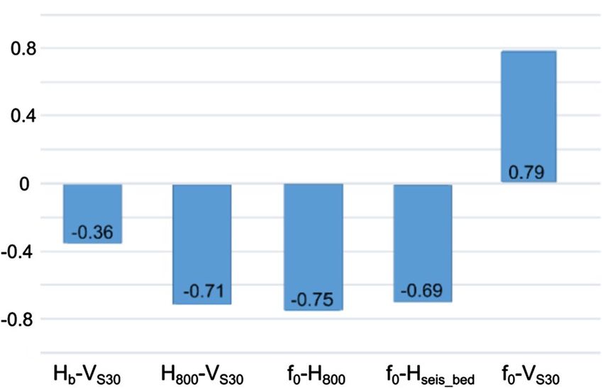
Bulletin of Earthquake Engineering

and the latter can be derived from the VS profile. However, another task of the same SERA
Project (Bergamo et al. 2019; 2021) adopted a regression analysis and a neural network
approach, to find the correlation between direct and indirect proxies and the true amplifica-
tion computed at Swiss and Japan stations. Among the 7 indicators indicated by the Cul-
trera et al. (2021), Bergamo et al. (2021) did not consider geological information in their
analysis. They found that the actual amplification in the range 1.7–6.7 Hz exhibits a good
correlation with a combination of velocity profile (described through specific frequency-
dependent “quarter-wavelength” quantities: average velocity and impedance contrast), VS30,
bedrock depth and f0.
    In our methodology, the quality of a site characterization is expressed by the compu-
tation of a final overall quality index (Final_QI), which is a number ranging between 0
and 1 and accounting for the single indicator quality, its relevance for site characterization,
and the consistency between all the significant indicators. Specifically, Final_QI is derived
from the computation of three simple quality indices (QI1, QI2 and QI3). QI1 quantifies
the reliability of each individual indicator, QI2 combines the QI1 values from the indi-
vidual indicators available at a given site, and QI3 is aimed at evaluating the consistency
between couples of indicators. The principles of such quality metrics have been presented
and discussed during a dedicated workshop in Italy (Cultrera et al. 2019) gathering Euro-
pean and worldwide scientists.

2.1 Quality index 1 (QI1)

We propose a simple, common expression involving the different aspects of the quality
evaluation of a single indicator (QI1 hereinafter), based on (1) the suitability of the method
for acquisition and analysis, (2) the type of input data (direct measurements or derived
from proxies) and quality of the processing, and (3) the completeness of the site report.
   The quality index QI1 varies from 0 to 1 and is defined by the following expression:

                                                                                            (1)
                                    [(                )      ]
                             QI1 = aMS + bID ⋅ cMI ⋅ dRC ∕3

where factors aMS, bID, cMI and dRC are detailed below and summarized in Table 1,
together with some indication on how to evaluate them. The factors are given only dis-
crete values in order to limit subjective choices. The value 3 in the denominator is equal to
aMSmax + bIDmax ⋅ cMImax where the suffix max indicates the maximum values of the factors.

2.1.1 Factors in QI1

In Eq. 1, factor aMS is related to the “theoretical” reliability of the methods used for data
acquisition and analysis for deriving the value of the target indicator (the suffix MS stands
for “method suitability”). It is equal to 1 when assessed on the basis of peer-reviewed
papers or well-established guidelines, otherwise it is given a 0 value (Table 1). As an
example, in the case of f0, aMS = 1 when the applied methodology follows published peer-
reviewed papers or consolidated guidelines (e.g. Nakamura et al. 1989; Field and Jacobs
1995; SESAME 2004; Picozzi et al. 2005; Haghshenas et al. 2008; Molnar et al. 2018
among many others).
   Factor bID deals with the type of data or information used for evaluating the target indi-
cator (the suffix ID stands for “input data”). As one of the main objectives is to emphasize
the importance of direct measurements rather than inferred estimates, it is assigned a value
of 2 in case of dedicated, in-situ field experiments, and a 0 value whenever inferred, i.e.

13
Bulletin of Earthquake Engineering
Table 1 Values of the factors in Eq. 1 for the computation of QI1. The suffixes in the factors name MS, ID,
MI and RC stand for method suitability, input data, method implementation and report completeness
Factor Definition Possible Value Explanation
values
aMS Suitability of the method 0, 1 1 The method of acquisition and analysis for
for acquisition and estimating the target indicator is appropri-
analysis ate and documented through several peer-
reviewed papers
0 The method of analysis and acquisition is not
published
bID Type of input data 0, 2 2 Direct evaluation based on specific field data
0 The evaluation is based on inferred values
derived from indirect proxies (Bergamo
et al. 2019), from empirical relationships
or modeling
cMI Method implementation 0, 0.5, 1 1 Correct data acquisition, processing and
(Data acquisition, pro- interpretation
cessing and interpreta-
tion)
0.5 In case of partial/moderate confidence on
data acquisition, processing and interpreta-
tion
0 Although described in the report, the indica-
tor is not reliable because the data acquisi-
tion step, processing or interpretation are
not correct
dRC Completeness of the site 0, 0.5, 1 1 A well-documented report for the specific
report indicator is present
0.5 A report associated to a site is present, but
the information is incomplete and insuf-
ficiently detailed
0 The value of indicator is provided without
any documentation related to it
obtained from proxies or empirical relationships (Table 1). Almost all funding agencies
favor the installation of seismic instruments neglecting the issue of the metadata quality,
which is however critical for data analysis. That is why the factor bID is given a binary
value 2 for actual measurements, and 0 for simply inferred values. For example in case
of f0, spectral ratios from single-station (either noise or earthquake recordings) measure-
ments are considered a direct evaluation (bID = 2), whereas the evaluation of f0 from 1D site
response modelling only (i.e., when 1D models are not constrained by specific field meas-
urements) is considered inferred (bID = 0). If the target indicator is the VS profile, invasive
measurements (such as downhole, crosshole, PS-logging whatever the investigation depth)
or not-invasive extensive field measurements (e.g. based on the inversion of surface-wave
dispersion properties) are considered as a direct evaluation (bID = 2). For the same consid-
eration, bID is 2 if VS30 is resolved by in-situ measurements. For the sake of simplicity, we
also suggest bID = 2 when VS30-VSZ relationships are used (e.g. Boore et al. 2011; Dai et al.
2013), with the reliability of the estimated VS30 being translated in factor c MI as described
later. If the target indicator is the near-surface geology, a geological field survey at the sta-
tion site or a detailed cartography (scale finer or equal to 1:10.000) is considered a direct
13Bulletin of Earthquake Engineering
evaluation (bID = 2). When the surface geology is derived exclusively from large scale car-
tography (i.e. 1:100.000) then bID is assigned equal to 0.
Factor cMI indicates the reliability of the indicator value in relation to the quality of data
acquisition, processing and interpretation (the suffix MI stands for the “method implemen-
tation” of the selected approach; Table 1). Typically, the quality of the in-situ measure-
ments may be assessed on the basis of the compliance with standard and robust procedures,
including the performance and suitability of the used equipment, while the quality of the
processing should account for the observance of commonly accepted guidelines, including
the proper interpretation of the final results. Depending on the degree of correctness, the
factor cMI can be equal to 0 (incorrect), 0.5 (partially correct) and 1 (correct). From Eq. 1,
the cMI value is obviously irrelevant when the factor bID of Eq. 1 is equal to zero (absence
of any direct measurements). Published review papers or guidelines can be used to judge
the precision of the analysis. For example, the f0 from single-station noise measurements
can be verified through the SESAME (2004) or others criteria (Picozzi et al. 2005), taking
into account the sensor cut-off frequency used in the field, the time-window length and
number of cycles selected in the analysis step with respect to f0, the amplitude and narrow-
ness of the spectral peak etc. In case of VS30 indicator, the factor cMI is set equal to 1 when
the relationships between VS30 and different time-averaged velocity VSZ at given depth z are
applied (Boore et al. 2011; Régnier et al. 2014; Wang and Wang 2015), assuming that such
relationships are calibrated for the studied area. In the estimation of shear-wave velocities
at larger depth, the uncertainties of these region-specific relationships obviously increase
when the maximum depth of the data is very limited (e.g. for z = 5, 10, 20 m). Because
of the large uncertainties, we recommend to set cMI = 0.5 when z is less than 15 m (Boore
et al. 2011; Kwak et al. 2017). Note that the evaluation of factor cMI can take advantage
from the summary reports as described in Cultrera et al. (2021), where the basic informa-
tion of data processing is collected in a compact form.
Factor dRC is related with the quality of the available documentation reporting the data
acquisition and processing (the suffix RC stands for “report completeness”): the maximum
value of 1 is for a complete report (see companion paper for the necessary information),
the intermediate value 0.5 is when partial information is present, whereas the absence of
a report leads to a dRC value of 0 (Table 1). The presence of a report is very important in
Eq. 1, because QI1 is equal to zero in case of absence of any report, even though there
might exist actual measurements followed by a correct interpretation.
The functional form of the generic Eq. 1 includes one addition and two multiplications,
which were deliberately introduced with the following rationale:
• Multiplication by a factor that may be equal to 0 indicates that whatever the value of
the other term of the multiplication, the absence or poor reliability will affect the whole
QI1 term. The product “bID · cMI” may thus be zero in case of absence of site-specific
direct measurements (bID), or in case of very inadequate acquisition or processing (cMI).
Similarly, the quality of the documentation (dRC) will drastically impact the QI1 what-
ever the relevancy of the methodology (aMS), the type of data (bID) and of the method
implementation (cMI). The absence or poor quality site documentation greatly hampers
the ability of external users to evaluate the indicator’s quality.
• Addition in Eq. 1 makes the factor aMS relatively independent from bID and cMI. For
instance, when VS30 is inferred from local slope or geology, aMS may be equal to 1
because the methodology has been published and is commonly accepted, while bID is
zero because the derivation is not based on direct measurements but from statistical
correlations with very large scatter.
13Bulletin of Earthquake Engineering
It is worthy of note that in the QI1 evaluation a careful examination of the available site
information in the proximity of the selected station is needed. Among the factors of Table 1
contributing to the QI1 definition, the one which is more difficult to judge is probably the
factor cMI. Specifically, factor cMI takes into account criteria on reliability of the used meth-
ods (including their resolution and commonly admitted rules-of-thumb), and appropriate
usage of empirical relationship available in literature when indicators are inferred (exam-
ples of empirical relationships are VS30-surface topography, Wald and Allen 2007; VS30-
VS10, Boore et al. 2011; VS30-phase velocity at 40 m wavelength; Martin and Diehl 2004).
The QI1 assignment should be as much as possible independent from subjective choices,
but the factor cMI could be biased by personal judgment. In order to reduce such bias for
each of the seven site indicators, we believe an expert judgment is necessary in the QI1
assessment; the quality evaluation should be in the responsibility of the analysis team and/
or of the network operators involved in site characterization.
2.1.2 QI1 examples
To better explain the effect on the different factor’s choices, we simulate the QI1 computa-
tion of f0 as target indicator and for virtual sites with the following characteristics (Table 2):
Site #1—f0 evaluated from horizontal-to-vertical (H/V) spectral ratios on ambient noise
data (bID = 2) evaluated following the SESAME (2004) guidelines (aMS = 1). The process-
ing is done with the Geopsy code (Wathelet et al. 2020) and a clear H/V peak occurs in the
frequency range within the applicability limits of the method (cMI = 1). A complete report
exists describing the field activity and data analysis (dRC = 1). All the factors of Table 1
take their maximum value as the resulting QI1 (QI1 = 1).
Site #2—f0 evaluated as a proxy from VS profile (bID = 0) following the simplified
approaches described in Dobry et al. (1976) or Wang et al. (2018) (aMS = 1). There are
uncertainties on the layered velocity profile used to derive the f0 value (cMI = 0.5): in this
case the value of factor cMI is irrelevant for the computation of QI1 because bID = 0 (see
Eq. 1). A detailed report exists describing the analysis (dRC = 1). The resulting QI1 is equal
to 0.33.
Site #3—as for site #1 but without any report (dRC = 0). QI1 is equal to its minimum
value (QI1 = 0).
Site #4—as for site #1 but the processing or interpretation of the final results is eval-
uated incorrectly (cMI = 0); this happens for example when f0 doesn’t indicate the fun-
damental peak but a secondary peak at higher frequency, or in case of the time-window
length too short to allow a robust estimation of f0. QI1 is equal to 0.33.
Site #5—as for site #1 but there is partial confidence in the processing or interpreta-
tion of the final results (cMI = 0.5). QI1 is equal to 0.67.
Site #6—All the factors reach the maximum value, except dRC because the site report
is considered not complete (dRC = 0.5). QI1 is equal to 0.5.
Site #7—Factors aMS and bID have the maximum values, but the processing or inter-
pretation are not correct (cMI = 0) and the site report is incomplete (dRC = 0.5). QI1 is
equal to 0.167.
In the next three examples (from #8 to #10 in Table 2), we assume that the target
indicator is the VS30 derived from a measured shear-wave velocity profile (aMS = 1 and
bID = 2). It is important to highlight that the maximum depth of investigation can be
confined in real situations to a very shallow depth (i.e. < 30 m):
13Bulletin of Earthquake Engineering
Table 2 Example of QI1 Site aMS bID cMI dRC QI1 (Eq. 1)
computation at ten sites. The
examples from #1 to #7 are
#1 1 2 1 1 1.00
referring to f0 as target indicator,
the examples from #8 to #10 #2 1 0 0.5 1 0.33
are referring to VS30 as a target #3 1 2 1 0 0
indicator (see text) #4 1 2 0 1 0.33
#5 1 2 0.5 1 0.667
#6 1 2 1 0.5 0.5
#7 1 2 0 0.5 0.167
#8 1 2 1 1 1.00
#9 1 2 0.5 1 0.667
#10 1 2 0 1 0.33
Site #8—VS30 was calculated using a downhole (DH) test near the seismic station. In
this example the DH test is with a maximum depth of 20 m, this is why a relationship
between VS20 and VS30 was used (for example Boore et al. 2011, factor aMS = 1). In this
case, the DH is a direct measurement (bID = 2) although limited in depth, and the appli-
cability of relationship VS20–VS30 is reliable (cMI = 1) because the station is located in
the region where the relationship was validated. A complete report exists describing the
field activity and data analysis (dRC = 1). All the factors of Table 1 take their maximum
value and QI1 is 1.
Site #9—Similar to site #8, but the maximum depth of the available DH survey
reaches only 5 m, and a relationship between VS5 and VS30, developed for the area of
analysis, was used (aMS = 1). Although the DH is very limited in depth, we consider it as
direct measurement (bID = 2) but, because the relationship may lead to large uncertainty,
the factor cMI is set equal to 0.5. The resulting QI1 is 0.667.
Site #10—Similar to site #9, except that the station is located in a region where the
VS5–VS30 relationship was never calibrated: aMS (published methods), bID (direct meas-
urements), dRC (presence of a full report) have their maximum values but cMI is set equal
to 0. QI1 is equal to 0.33.
Table 2 summarizes the factors and the resulting QI1 computed for the 10 sites. QI1 can
have six possible values (0, 0.167, 0.33, 0.5, 0.667 and 1) that are connected to the reli-
ability of each single indicator and can be interpreted in terms of quality as: unreliable (0),
very poor (0.167), poor (0.33), acceptable (0.5), good (0.67) and very good (1).
The absence of a report (dRC = 0) implies QI1 equals to zero (e.g. site #3). Another sig-
nificant factor is bID: without direct measurements (bID = 0; e.g. site #2) QI1 cannot exceed
the value of 0.33. The same QI1 value of 0.33 is reached in case of direct measurements
(bID = 2) but with the method implementation having some problem (cMI = 0; e.g. site #4).
Although the definition of QI1 in Eq. 1 is aimed at penalizing the lack of a report and
the use of proxies or empirical relationships, the absence of a direct measurements (i.e.
bID = 0) does not give necessarily a QI1 equal to zero, as shown from the above examples.
Strong-motion databases, like the Italian one, lack of in-situ measurements at the recording
station, but they usually adopt peer-reviewed methods (aMS = 1) which are properly imple-
mented (cMI = 1) and fully described in a report (dRC = 1).
Other examples of how to select the proper value for factor aMS, bID and cMI are reported
in the "Appendix" materials ( "Appendix" Tables 7, 8 and 9) and in Bergamo et al. 2019
(see their Tables 1, 2, 3, 4, 5). This auxiliary material provides indications on how to assign
13Bulletin of Earthquake Engineering
the factors that appear in Eq. 1, but is not exhaustive of all situations that may be encoun-
tered by analyzing real sites.
2.2 Quality index 2 (QI2)
Once the QI1 is computed for each indicator through Eq. 1, QI2 is evaluated as a weighted
sum of the QI1 of all indicators at the target site:
[ ]
∑ ∑
QI2 = wi ⋅ QI1i ∕ wi (2)
i=1,n i=1,n
where wi is the weight relative to the i-th indicator and n indicates their total number. In
this paper n is equal to 7, i.e. the number of indicators considered as most appropriate fol-
lowing the companion paper (Cultrera et al. 2021). If some of the indicators are not avail-
able at the target site, its corresponding QI1i is equal to zero in Eq. 2. In detail, QI2 varies
from 0 to 1, and it cares for the importance of the indicators on the evaluation of the site
characterization through the weights wi. Because QI1 can assume six discrete values, the
choice of weights in the definition of QI2 should ensure a wider and gradual distribution
of the QI2 values, depending on the number and importance of available indicators at each
site. The weights must take into account the relevance of the selected indicators in the site
characterization and, after testing various options for the selection of wi values (Di Giulio
et al. 2019), we propose three simple weight classes (Table 3) according to the indication
provided by the survey described in the companion paper:
• A maximum weight of 1 for f0 and velocity profile VS. These two indicators were the
most recommended indicators (72% and 89% respectively; see Table 3) to be used for
site metadata, and they are directly linked to the dynamic soil properties and to soil
amplification.
• An intermediate weight of 0.5 for the indicators VS30, engineering and seismological
bedrock depth, surface geology. In this group, surface geology has a qualitative rela-
tion with site effect estimation, and VS30 or bedrock depth can be derived from veloc-
ity profile VS and f0. This group of indicators were considered as mandatory by the
participants to the online questionnaire in a percentage ranging between 55 and 63%
(Table 3).
Table 3 Weights of the relevant indicators for computation of QI2 (Eq. 2). The last column indicates the
number of the answer (in percentage) to the online questionnaire indicating the indicator as mandatory (see
Fig. 3 of the companion paper Cultrera et al. 2021)
Indicator Weight wi Mandatory (%)
f0 1 89
VS30 0.5 63
Surface geology 0.5 61
Shear-wave velocity profile (VS) 1 72
Depth of seismological bedrock (Hseis_bed) 0.5 58
Depth of engineering bedrock (H800) 0.5 55
Soil class 0.25 56
13Bulletin of Earthquake Engineering
• A minimum weight of 0.25 for the “soil class” indicator. Although this indicator had
the same percentage of ‘mandatory’ attribution of the previous group (Table 3), we
assigned the lowest value because it is an indirect proxy for site conditions, derived
mostly from the other indicators already considered in the weighted average (such as
VS30, engineering bedrock depth and geology).
Unlike the QI1 evaluation, QI2 can be computed automatically applying Eq. 2 and
it does not require any other analysis from the operator. To illustrate the QI2 index, we
computed Eq. 2 at virtual sites characterized by different combinations of the recom-
mended indicators (Fig. 1). For the sake of simplicity, we considered three possible values
of QI1: 1, 0.5 and 0. These values were mutually assumed by the seven indicators. The
null value of QI1 in Eq. 2 implies the absence of an indicator or the lack of a report. We
then decreased gradually the number of the available indicators from 7 to 1, and sorted the
results in decreasing order (Fig. 1). The ranking is from the maximum value of 1 (all the
seven indicators are available with QI1 = 1) to the lowest value (only VS30 or geology are
available with a QI1 equals to 0.5). The QI2 trend (Fig. 1) is clearly related to the number
of the indicators, and to their relevance for site characterization analysis according to the
weights of Table 3. The red circles with letters in Fig. 1 indicate five virtual sites: at site A
(QI2 = 1) the seven indicators are all available with a QI1 of 1; at site B (QI2 = 0.38) the
available indicators are four (f0, surface geology, VS30 and soil class) and f0 is with QI1 = 1
whereas the others have QI1 = 0.5; at site C (QI2 = 0.35) the available indicators are two
(VS30 and VS profile with QI1 = 1); at site D (QI2 = 0.09) the indicators are two but with
lower weight (surface geology and soil class with a QI1 = 0.5); at site E (QI2 = 0.06) the
only indicator is VS30 with a QI1 = 0.5. Other combinations of the indicators may return the
same QI2 value of the above examples, as shown in the auxiliary material ( "Appendix"
Table 10).
It is worth noting that QI2 compensates the possible overestimation of the QI1 of some
indicator. This is the case of the site #9 in Table 2, for which the QI1 of the VS30 indicator
may appear likely overestimated (QI1 = 0.67) because of the use of the VS5–VS30 relation-
ship. However, because of the very limited depth of 5 m of the DH measurements, there are
chances that QI1 values for the other indicators (H800, Hseis_bed and soil class) would be low,
Fig. 1 QI2 values for various sets of indicators. The red circles with letters indicate five virtual sites (see
text). The full computation of the histograms is reported in the auxiliary material (see table 10 in “Appen-
dix”)
13Bulletin of Earthquake Engineering
and as consequence QI2 is also expected to be low. Only in case of a bedrock site, with few
meters (< 5 m) of weathered outcrop over stiff rock, H800 and Hseis_bed can be intercepted
within the first 5 m, and the associated QI2 value gets consistently a relatively high value.
2.3 Quality index 3 (QI3)
QI3 is aimed at evaluating the consistency of various pairs of indicators that are related to
each other. It is expressed by the following equation:
[ ]
∑
QI3 = csk ∕m (3)
k=1,m
where csk is the consistency factor for a pair of indicators identified by k, and m is the num-
ber of available couples of indicators at the specific site. The consistency factor csk can be
either 0 (no consistency) or 1 (consistency), and the QI3 is ranging from 0 to 1. QI3 has
a physical meaning because it represents the proportion of the selected pairs of indicators
that are consistent with one another.
In our proposal, out of the 7 recommended indicators, we fixed the number of possible
pairs to 5 (m equals to 5). This is because 5 is the number of pairs of indicators which have
been measured for a large enough dataset to allow reliable relationships through scatter
plots. The five pairs are: f0 & VS30 (k = 1), f0 & seismic bedrock depth (k = 2), f0 & engi-
neering bedrock depth (k = 3), VS30 & engineering bedrock depth (k = 4) and VS30 & geol-
ogy (k = 5). The value of csk at a specific site is set equal to 0 if one or both indicators of
the pair k are not present.
Empirical relationships between various indicators can be found in the form of scat-
ter plots in scientific literature for evaluating the consistency between indicators. Several
papers propose empirical relationships between pairs of indicators to investigate the ability
of different indicators in characterizing site response, or their use for a suitable definition
of the amplification factors within seismic codes (Boore et al. 2014; Kamai et al. 2016;
Stambouli et al. 2017). As an example, in the following we list a selection of papers show-
ing correlations for the five pairs considered in Eq. 3:
(1) f0—VS30 (e.g. Luzi et al. 2011; Gofhrani and Atkinson 2014; Régnier et al 2014; Has-
sani and Atkinson 2016; Derras et al. 2017; Stambouli et al. 2017; Zhu et al. 2020);
(2) f0—seismic bedrock depth (e.g. Ibs-Von Seht and Wohlenberg 1999; Parolai et al. 2002;
Hinzen et al. 2004; Gosar and Lenart 2009; Luzi et al. 2011);
(3) f0—engineering bedrock depth (H800) (e.g. Derras et al. 2017);
(4) VS30—engineering bedrock depth (H800) (e.g. Derras et al. 2017; Piltz and Cotton 2019;
Zhu et al. 2020; Bergamo et al. 2021);
(5) VS30—surface geology (e.g. Wills et al. 2000 and 2015; Wald and Allen 2007; Lemoine
et al. 2012; Stewart et al. 2014; Yong et al. 2016; Derras et al. 2017; Foti et al. 2018;
Ahdi et al. 2017; Mital et al. 2021).
Such empirical relationships generally refer to a specific database, and several checks
are needed to ensure the applicability to the site under study. First, it is important to
check the homogeneity of the analysis at the base of such relationships, and if the defi-
nition of the indicators is exactly the same (e.g. “peak” or “fundamental” frequency,
13Bulletin of Earthquake Engineering
derived from H/V spectral ratios of 5% damped pseudo spectral acceleration, or from
Fourier Amplitude Spectra, etc.). Second, the relationships might be variable from
region to region. Therefore, the consistency evaluations should, as much as possible,
take into account the available studies for the areas including or neighboring the target
station.
In order to avoid being stuck to a given region or database, we propose in the present
paper a reference set of scatter plots (for the selected five pairs of indicators) to compare
with the measured value at a specific site and evaluate csk in Eq. 3. When the indicators
are within or out of the confidence interval of our scatter plots, we set csk equal to 1 or
0, respectively.
We first selected 935 sites where real VS profiles are accessible, and we then homoge-
neously computed the other indicators assuming a 1D velocity model. Soil class, depth
of engineering bedrock (H800) defined as the depth where shear-wave velocity is equal
or first exceeds the conventional EC8 (CEN 2004) value of 800 m/s, VS30 and theoretical
f0 from SH amplification were evaluated using the reflectivity method (Kennet, 1983),
whereas the seismic bedrock (Hseis_bed) came from the depth for which the resonance
frequency, provided by simplified Rayleigh’s method (Dobry et al. 1976), is close to the
value of the measured f0. The VS profiles were selected from 935 real sites: 602 are from
Kiknet network (http://www.kyoshin.bosai.go.jp/), 243 from California (Boore, 2003;
http://quake.usgs.gov/~boore), 21 from European strong-motion sites (Di Giulio et al.
2012), 33 from French (Hollender et al. 2018), and 36 are Italian sites from ITACA
database (D’Amico et al. 2020). The complete list of the 935 stations is given in Di
Giulio et al. (2019). The maximum depth of investigation is 600 m, but the majority of
the sites does not exceed the depth of 300 m. For 15 profiles having shear-wave velocity
larger than 800 m/s starting from the surface, we set H800 equal to 1 m. A number of 18
sites within the analyzed profiles never reach a shear-wave velocity of 800 m/s.
Scatter plots for the different pairs of indicators are shown in Fig. 2: f0 & VS30; f0 &
Hseis_bed; f0 & H800; and H800 & VS30. As expected, the seismic (Hseis_bed) and the engi-
neering (H800) bedrock depths are inversely proportional to f0: the deeper the seismic
interface, the lower the corresponding resonance frequency (Fig. 2b, c). VS30 is increas-
ing with f0 (the softer the surface layer, the lower the resonance frequency; Fig. 2a), and
is decreasing with increasing H800 (the softer the surface layer, the deeper the engineer-
ing bedrock depth; Fig. 2d).
Spearman’s rank correlation coefficient (Spearman, 1904) was also computed between
each pair of indicators used in the scatter plots. This coefficient (Fig. 3) describes how
well the relationships in the scatter plots can be described by a monotonic function, and
the sign of the coefficient reflects the direction of the relationships between indicators. The
histograms of Fig. 3 show that the highest degree of correlation is shown by the pair f0-VS30
(coefficient equals to 0.79), which is the only one with a positive sign. The remaining pairs
show a Spearman’s correlation coefficient fairly high (from 0.69 to 0.75 as absolute value),
except the pair Hseis_bed-VS30 that shows the lowest value (− 0.36).
However, the plots of Fig. 2 show a larger scatter, together with a shortage of data
(i.e. few samples) at low frequencies (panels a, b, c). They thus cannot be considered
representative for deep sites, i.e. when f0 is less than 0.3 Hz or when the depth of the
stiff interface (Hseis_bed or H800) is larger than 200 m, because of the limited number of
samples in our data set. A large scatter is also observed in the high-frequency (> 10 Hz)
range in the f0—Hseis_bed scatter plot (Fig. 2b), where Hseis_bed varies from a few meters
up to 100 m.
13Bulletin of Earthquake Engineering
Fig. 2 Scatter plot for the pairs of indicators: a f0-VS30, b f0-seismic bedrock depth, c f0-H800, d H800-VS30.
The gray circles show the values computed at 935 sites, the square symbols indicate the values at the real
sites listed in Table 4. The geometric mean and the mean ± 2 standard deviation are computed assuming
logarithmic bins along the x-axis and they are reported as black thick and thin lines, respectively. The mean
curves and associated variability are given in the "Appendix" material ("Appendix" Tables 17, 18, 19 and
20)
From the plots of Fig. 2, we assume that the consistency between a pair of indicators
is quantified in a binary way depending on whether or not it falls within the confidence
interval given by ± 2 standard deviations around the geometric mean (black lines in
Fig. 2): we precautionary assume csk = 1 when the values of a site is within this range.
As shown in Fig. 2, the resonance frequency f0 is a very important indicator in our
strategy and is therefore present in three over four scatter plots of Fig. 2. However, in
case of a site that does not show a resonance peak, the scatter plots of Fig. 2a, b, c can-
not be used to verify the consistency between indicators. This is why csk in Eq. 3 can
be assumed equal to 1 (for k = 1,2,3) even when a site does not show a resonance peak
(e.g. flat H/V curves), but is classified as a stiff soil or bedrock site from geological and
geophysical consideration (Pilz et al. 2020; Lanzano et al. 2020).
13Bulletin of Earthquake Engineering
Fig.3 Spearman’s correla-
tion coefficient for the pairs of
indicators
Regarding the consistency between VS30 and surface geology, we recommend to check
it by using the velocity ranges associated to the different lithological groups listed in lit-
erature data or based on regional VS30—surface geology relationships (if available). Spe-
cifically, some reference range of shear-wave velocity for different European soils (soft and
stiff clay, loose and dense sand, gravels) and rocks (weathered and competent rocks) can
be found in Foti et al. 2018 (Table 3 in their work). Other indication of the expected VS30
for different geological categories (on the basis of age, grain degradation and depositional
environment) are reported in Stewart et al. (2014) for Greece, in Parker et al. (2017) for
Central and Eastern North America, in Xie et al. (2016) for China area, in Michel et al
(2014) for Swiss sites and Mital et al. (2021) for different terrain classes in United States.
For Italy, Forte et al. (2019) proposed a soil classification considering 20 geological-lith-
ological complexes; they made available a stand-alone software for database interrogation
that gives the median and standard deviation of VS30 after defining the coordinates of the
site. All these studies dealing with VS30 and surface geology depend from a starting soil-
profile database built on site-specific measurements, and then extrapolated to a large scale
using geological information or terrain map-based models including topographic slope or
geomorphic terrain classifications (Yong 2016). It is also possible to have values of VS30
at a finer spatial scale using available observations from previous studies performed in the
area where the station is located, e.g. information from microzonation activities (such as
Amanti et al. 2020 for the Central Apennine or Saroli et al. 2020 at municipal scale), or
from existing geotechnical-engineering database (Passeri et al. 2021).
Studies investigating the distribution of VS30 are still few (Mital et al. 2021), and almost
all the works cited above give a mean value of VS30 for a certain geological-lithological
layer, with the uncertainty that are expressed as standard deviation or through a range
within a minimum and maximum value. For evaluating csk between VS30 and surface geol-
ogy, especially in case of regional relationships, we suggest in a precautionary way to
select as velocity uncertainty two standard deviations, or the full range between the mini-
mum and maximum value in the provided distribution.
In the QI3 computation, we didn’t consider the VS30 & Hseis_bed pair because the shallow
depth limitation of VS30 makes its relationship to the seismic bedrock depth meaningful
only when the stiff interface is very shallow (i.e. at a depth < 30 m). The scatter plot of this
pair of indicators is actually shown in Fig. 4 and displays a very large variability over the
entire range of x- or y- axis, consistently to the low value of Spearman’s correlation.
13Bulletin of Earthquake Engineering
3 Quality metrics computation at real sites
Once the three quality indices (QI1, QI2 and QI3) are computed, the final quality index
(Final_QI) for the overall characterization of a site is conclusively computed as arithmeti-
cal average between QI2 and QI3:
Final_QI = [QI2 + QI3]∕2 (4)
As previously described, QI2 accounts for the presence of the relevant indicators (Eq. 2)
and QI3 for the consistency of their values (Eq. 3). The range of Final_QI is spanning from
0 to 1: a value of 1 is assigned to a site with a detailed and good seismic characterization, 0
is for a site poorly or not characterized.
We verify this quality procedure by applying it to seven seismic stations (Table 4)
of two permanent seismic networks of Italy: INGV National seismic network (network
code IV; https://doi.org/10.13127/SD/X0FXnH7QfY) and the strong-motion network
operated by Presidency of Council of Ministers-Civil Protection Department (network
code IT; https://doi.org/10.7914/SN/IT). The soil class of the investigated stations
(Table 4) following the EC8 seismic code (CEN 2004) is B or C; these are the most
common classes for sites of the seismic networks in Europe (Felicetta et al. 2017).
The location of the seven sites and the information on their site characterization are
available online through public reports at the Italian Accelerometric Archive (ITACA;
http://itaca.mi.ingv.it; D’Amico et al. 2020) and at the Engineering-Strong Motion data-
base (ESM; https://esm-db.eu; Luzi et al. 2020). The geological and geophysical reports
can be downloaded from the stations section of these databases. Table 4 shows the
available indicators extracted from the reports; the corresponding values are also plot-
ted in the scatter plots of Fig. 2 as squared symbols. All the sites of Table 4, with the
exception of IT.CSM, have several information provided from ad-hoc geophysical and
geological surveys carried out within recent national projects for site characterization of
permanent networks (e.g. Bordoni et al. 2017; Cultrera et al. 2018) or from microzoning
studies. IT.PNG has partial information due to the lack of direct measurements of shear-
wave velocity profile in proximity of the station, and VS30 is inferred by correlation with
Fig. 4 Scatter plot for the couple Hseis_bed-VS30. The color scale is proportional to the soil class category, fol-
lowing the classification of EC8 building code (CEN 2004)
13Bulletin of Earthquake Engineering
Table 4 List of indicators extracted at seven real sites from the available reports
Station f0 Hseis_bed H800 VS30 VS Surface geology Soil class
(Hz) (m) (m) (m/s) (m/s) (based on
EC8)
IV.ROM9 1 173 (amv) 6 (CH) 605 (CH) (CH) geological survey B
14 (DH) 532 (DH) (DH) map 1:5000
173 (amv) 414 (amv) (amv)
(Fig. 5)
IV.CDCA 0.4 140 (well) 140 (well) 275 (amv) (amv) well and geological C
184 (amv) 184 (amv) survey
map 1:5000
IV.LAV9 2.3 125 (gm) 125 (gm) 286 (amv; (amv; geological survey C
48 (amv; 48 (amv; masw) masw) map 1:5000
masw) masw)
IT.ORC 1.3 24 (amv) 24 (amv) 767(amv) (amv) geological survey B
map 1:5000
IT.MCA none Outcrop 29 (amv; 530 (amv; (amv; geological survey B
(flat masw) masw) masw) map 1:5000
H/V)
IT.CSM none none none none None geological map B
1:100,000 (geology)
IT.PNG 0.54 45 (mzs) none 418 (topog- None geological map C (mzs)
raphy) 1:5000
The methods used to measure the indicators are indicated in parenthesis: ‘amv’ means array inversion based
on ambient vibration passive data; ‘masw’ is array analysis using an active source; ’DH’ and ’CH’ means
downhole and crosshole survey; ‘gm’ stands for geological model; ‘mzs’ for microzoning studies
topography (https://esm-db.eu; Luzi et al. 2020) and soil class by first-level microzona-
tion study (Zarrilli and Moschillo 2020).
We detail below the step-by-step quantitative quality assessment at IV.ROM9. Many
geophysical measurements were performed at this site for recovering the local velocity
profile, such as down-hole (DH) and cross-hole (CH) tests (up to 70 m deep; Cercato
et al. 2018), and 2D passive surface-wave array experiments, together with a geological
map based on ad hoc field survey (Bonomo et al. 2017). The 2D passive array analysis
should be considered as independent from invasive surveys because it was done before
the profiles from DH and CH were made public. As an example of the information avail-
able at IV.ROM9, Fig. 5 illustrates a set of H/V noise spectral curves (panels a and
b), the comparison of the velocity profile VS obtained from different methods (panel c)
and the geological map (scale 1:5000) in panel d. A total of 36 points of noise meas-
urements of a few hours, through three 2D passive arrays of increasing spatial aper-
ture around the location of IV.ROM9, showed consistently a resonance frequency at
1 Hz (see Fig. 5b). This ensures the spatial stability of the 1 Hz peak, which is also
stable with time (Fig. 5a), with a possible additional and weaker peak also at 0.4 Hz. In
the next of the quality evaluation, we consider the f0 value of IV.ROM9 equal to 1 Hz
(Fig. 5b). Three different VS profiles (Fig. 5c) are available from direct measurements
but none of them was indicated at the best model before our analysis. The “amv” model
shows i) a deeper interface, with a velocity contrast of about 2, at about 170 m that is
related to the f0 peak at 1 Hz, and ii) a lower velocity at the surface in comparison to the
profiles obtained by invasive methods (Fig. 5c). It is not so uncommon to get different
13Bulletin of Earthquake Engineering
VS profiles by using different data and techniques, especially when data are collected at
different times and analyzed by different teams in a blind way. In general, amv methods
based on surface-wave analysis can provide lower velocities in the uppermost part of the
profile with respect to DH and CH surveys (Passeri et al. 2021). This discrepancy may
be related to the grouting hole operations, to the different volumes investigated by the
methodologies, and to the lower resolution of surface-wave methods in resolving very
thin layers. As authoritative choice of the best VS profile, we considered a combined
one, obtained by the CH up to a depth of 70 m (the invasive method which is considered
as the most reliable for the near-surface part; Di Giulio et al. 2018), and by the joint
surface-wave amv model that is characterized by a deeper investigation capability (inset
of Fig. 5c). In similar cases, when more measurements for the same indicator are avail-
able, it is recommended that the authoritative solution, obtained by expert judgement, is
indicated in the seismic databases collecting information for the stations together with a
synthesis report.
QI1 evaluation at IV.ROM9 of each indicator is summarized in Table 5, together with an
explanation of the chosen values. Three indicators (f0, surface geology and soil class) give
a QI1 equal to 1, i.e. the maximum value, meaning that they have been computed with reli-
able methods (factor aMS = 1 in Eq. 1), direct measurements (bID = 2), confident estimates
(cMI = 1) and well documented reports (dRC = 1). One of the SESAME (2004) criteria uses
a threshold of 2 in the H/V peak amplitude (assuming a squared average of the horizontal
components in the H/V analysis). The amplitude peak is not above 2 for all the 36 points
of noise measurements at IV.ROM9, although very close to this threshold value (Fig. 5b).
For the indicator f0 the factor cMI, which is connected to the proper method implementation
and interpretation of the results, was evaluated equal to its maximum value (cMI = 1) due to
the consistent shape of the H/V curves around 1 Hz (Fig. 5b), and to the spatial and time
stability of the H/V peak obtained from multiple measurements.
The remaining four indicators have a lower QI1 value: 0.67 for VS, VS30 and Hseis_bed,
0.33 for H800. This is related to the factor cMI which was set to 0.5 for both VS, VS30 and
Hseis_bed considering the discrepancies observed in the velocity profiles (Fig. 5c), and equal
to 0 for H800 (Table 4).
Concerning the VS30 value, the measurements return 532 m/s for down-hole survey
(DH), 605 m/s for Cross-Hole test (CH) and 414 m/s for surface-wave inversion of passive
data (Table 4). Each method is considered a direct measurement (factor bID = 2) and has its
own resolution in resolving thin layers (Fig. 5c), and the surface-wave inversion was per-
formed independently with respect to the invasive methods. Such discrepancy in the VS30
value is also due to the presence of a velocity inversion that is identified by the CH and DH
methods, which was not considered during the model parameterization in the surface-wave
array analysis, and to the difference between areal and discrete measurements. For these
reasons the factor cMI of the VS30 indicator was set equal to the intermediate value of 0.5.
About the seismic bedrock (Hseis_bed), the surface-wave analysis only is able to find it at
a depth of about 170 m (Fig. 5c). However, the factor cMI relative to Hseis_bed was set equal
to 0.5 (Table 5). This because the assumption of considering the H/V as Rayleigh-wave
ellipticity during the inversion step of analysis, not including the possible bias from Love
or body waves (Hobiger et al. 2009; Knapmeyer-Endrun et al. 2017), as well as the pres-
ence in the area of further H/V peaks at lower frequencies (Marcucci et al. 2019), needs to
be verified more in detail.
For the H800 indicator, the shear-wave velocity profile derived from surface-wave analy-
sis exceeds 800 m/s only in the deep basement layer (at a depth of 170 m), conversely the
CH and DH surveys exceed 800 m/s several times in the uppermost profile: the first time
13Bulletin of Earthquake Engineering
Fig. 5 IV.ROM9 station. a H/V noise spectral ratios using the continuous recording of IV.ROM9 (sensor
Trillium 120 s); the results of the first two months of 2015 are shown. H/V noise spectral ratios of the geo-
physical survey (sensor Lennartz 3d-5 s); the mean curves of 12 measurements (each of about 2 h of time
length; recording day 9 March 2017) are overlaid. c VS profile obtained through surface-wave inversion of
ambient vibration data (amv), from crosshole (CH) and downhole (DH). The inset shows the best velocity
profile obtained combining the CH and the amv model. d Geological map (scale 1:5000) after the field sur-
vey (Bonomo et al. 2017)
is at a depth of 6 m (CH) and 14 m (DH). The velocity value of 800 m/s is maintained for
very thin layers (Fig. 5c), while at the bottom of such layers the velocity returns to lower
values than 800 m/s. The factor cMI for the H800 indicator was set equal to 0 (Table 5) for
such discrepancy among the CH, DH and surface-wave profiles, too large even if we take
into account the lower resolution of the ambient vibration methods in solving thin surface
layers. However, H800 in the European code is defined as “the depth of the bedrock forma-
tion identified by shear-wave velocity larger than 800 m/s” and it is not specified if it is
the depth which it first exceeds 800 m/s (as assumed in this and companion paper), or the
depth below which the velocity is always larger than 800 m/s.
Finally, the cMI values indicated in Table 5 reflect the lack of consistency for certain
indicators (H800, VS30, VS) caused by the absence of a final site characterization summary
report which combines the various VS estimates providing an authoritative VS profile, e.g.
13Table 5 QI1 computation (Eq. 1) for the 7 recommended indicators at station IV.ROM9, together with the factor values and the indication on how they have been evaluated.
Similar tables for the other selected stations are shown in the "Appendix" (from "Appendix" Tables 11, 12, 13, 14, 15, 16)
Indicator Factor Value Notes
f0 aMS 1 f0 computed on H/V noise spectral ratios (www.geopsy.org; Wathelet et al. 2020)
bID 2 direct measurements of several ambient noise measurements repeated in time
cMI 1 the processing is correct (www.geopsy.org). The interpretation of H/V curve with a resonance at 1 Hz is
also correct; the f0 peak is consistent and stable with time and around the site, although the amplitude of
the H/V peak is sometime slightly lower than 2
Bulletin of Earthquake Engineering
dRC 1 complete geophysical report on noise measurements and f0 evaluation (available in ITACA website)
QI1 1
Surface geology
aMS 1 geological map at 1:5000 scale (Fig. 5c) based on a field survey and stratigraphical logs
bID 2 field survey
cMI 1 The geological survey was executed in proximity and around the station by a dedicated team of geologists
(Bonomo et al. 2017 and Fig. 5b)
dRC 1 complete geological report (available in ITACA website)
QI1 1
Soil class
aMS 1 from VS profile (by definition)
bID 2 computed directly from measured VS profiles
cMI 1 Soil class assignation, even if different VS measurements, is the same
dRC 1 complete report on VS profile measurements and soil class assignation in ITACA website
QI1 1
VS
aMS 1 DH + CH + 2D passive arrays with frequency-wavenumber FK analysis (http://www.geopsy.org)
bID 2 direct geophysical measurements: DH + CH and 2D array of seismic stations in passive configuration
cMI 0.5 DH, CH and array inversion gives different results, in the limits of their resolution. To account for this dis-
crepancy, we set cMI = 0.5. We then selected an authoritative VS profile combining CH and surface-wave
model (which are considered more suitable for the uppermost and deep part of the profile, respectively)
13
dRC 1 complete report on array, DH and CH measurements in ITACA websiteYou can also read