Citizen science flow - an assessment of simple streamflow measurement methods - HESS
←
→
Page content transcription
If your browser does not render page correctly, please read the page content below
Hydrol. Earth Syst. Sci., 23, 1045–1065, 2019
https://doi.org/10.5194/hess-23-1045-2019
© Author(s) 2019. This work is distributed under
the Creative Commons Attribution 4.0 License.

Citizen science flow – an assessment of simple streamflow
measurement methods
Jeffrey C. Davids1,2 , Martine M. Rutten3 , Anusha Pandey4 , Nischal Devkota4 , Wessel David van Oyen3 ,
Rajaram Prajapati4 , and Nick van de Giesen1
1 Water Management, Civil Engineering and Geosciences, Delft University of Technology, Building 23,
Stevinweg 1, 2628 CN, Delft, the Netherlands
2 SmartPhones4Water, 3881 Benatar Way, Suite G, Chico, California 95928, USA
3 Engineering and Applied Sciences, Rotterdam University, G.J. de Jonghweg 4–6, 3015 GG, Rotterdam, the Netherlands
4 SmartPhones4Water–Nepal, Damodar Marg, Thusikhel, 44600, Lalitpur, Nepal

Correspondence: Jeffrey C. Davids (j.c.davids@tudelft.nl)

Received: 7 August 2018 – Discussion started: 21 August 2018
Revised: 19 January 2019 – Accepted: 7 February 2019 – Published: 20 February 2019

Abstract. Wise management of water resources requires              sults, we selected salt dilution as the preferred method. Fi-
data. Nevertheless, the amount of streamflow data being col-       nally, we performed larger-scale pilot testing in week-long
lected globally continues to decline. Generating hydrologic        pre- and post-monsoon Citizen Science Flow campaigns in-
data together with citizen scientists can help fill this grow-     volving 25 and 37 citizen scientists, respectively. Observed
ing hydrological data gap. Our aim herein was to (1) per-          flows (n = 131 pre-monsoon; n = 133 post-monsoon) were
form an initial evaluation of three simple streamflow mea-         distributed among the 10 headwater catchments of the Kath-
surement methods (i.e., float, salt dilution, and Bernoulli run-   mandu Valley and ranged from 0.4 to 425 L s−1 and from 1.1
up), (2) evaluate the same three methods with citizen scien-       to 1804 L s−1 in pre- and post-monsoon, respectively. Future
tists, and (3) apply the preferred method at more sites with       work should further evaluate uncertainties of citizen science
more people. For computing errors, we used midsection mea-         salt dilution measurements, the feasibility of their application
surements from an acoustic Doppler velocimeter as refer-           to larger regions, and the information content of additional
ence flows. First, we (authors) performed 20 evaluation mea-       streamflow data.
surements in headwater catchments of the Kathmandu Val-
ley, Nepal. Reference flows ranged from 6.4 to 240 L s−1 .
Absolute errors averaged 23 %, 15 %, and 37 % with aver-           1     Introduction
age biases of 8 %, 6 %, and 26 % for float, salt dilution, and
Bernoulli methods, respectively. Second, we evaluated the          1.1    Background
same three methods at 15 sites in two watersheds within
the Kathmandu Valley with 10 groups of citizen scientists          The importance of measuring streamflow is underpinned by
(three to four members each) and one “expert” group (au-           the reality that it is the only truly integrated representation of
thors). At each site, each group performed three simple meth-      the entire catchment that we can plainly observe (McCulloch,
ods; experts also performed SonTek FlowTracker midsec-             1996). Traditional streamflow measurement approaches rely-
tion reference measurements (ranging from 4.2 to 896 L s−1 ).      ing on sophisticated sensors (e.g., pressure transducers and
For float, salt dilution, and Bernoulli methods, absolute er-      acoustic Doppler devices), site improvements (e.g., installa-
rors averaged 41 %, 21 %, and 43 % for experts and 63 %,           tion of weirs or stable cross sections), and discharge mea-
28 %, and 131 % for citizen scientists, while biases aver-         surements performed by specialists are often necessary at key
aged 41 %, 19 %, and 40 % for experts and 52 %, 7 %, and           observation points. However, these approaches require sig-
127 % for citizen scientists, respectively. Based on these re-     nificant funding, equipment, and expertise and are often dif-
                                                                   ficult to maintain, and even more so to scale (Davids et al.,

Published by Copernicus Publications on behalf of the European Geosciences Union.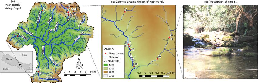
1046                 J. C. Davids et al.: Citizen science flow – an assessment of simple streamflow measurement methods

2017). Consequently, despite growing demand, the amount            Meerveld et al. (2017) showed that citizen science observa-
of streamflow data being collected continues to decline in         tions of stream level class can be informative for deriving
several parts of the world, especially in Africa, Latin Amer-      model-based streamflow time series of ungauged basins.
ica, Asia, and even North America (Hannah et al., 2011;               While the previously referenced studies focus mainly
Van de Giesen et al., 2014; Feki et al., 2017; Tauro et al.,       on involving citizen scientists for observing stream lev-
2018). Specifically, there is an acute shortage of streamflow      els, we were primarily concerned with the possibility of
data in headwater catchments (Kirchner, 2006) and devel-           enabling citizen scientists to take direct measurements of
oping regions (Mulligan, 2013). This data gap is perpetu-          streamflow. Using keyword searches with combinations of
ated by a lack of understanding among policy makers and            “citizen science”, “citizen hydrology”, “community mon-
citizens alike regarding the importance of streamflow data,        itoring”, “streamflow monitoring”, “streamflow measure-
which leads to persistent funding challenges (Kundzewicz,          ments”, “smartphone streamflow measurement”, and “dis-
1997; Pearson, 1998). This is further compounded by the re-        charge measurements”, we found that research on using
ality that the hydrological sciences research community has        smartphone video processing methods for streamflow mea-
focused much of its efforts in recent decades on advancing         surement has been ongoing for nearly 5 years (Lüthi et al.,
modeling techniques, while innovation in methods for gener-        2014; Peña-Haro et al., 2018). Despite the promising nature
ating the data these models depend on has been relegated to        of these technologies, we could not find any specific studies
a lower priority (Mishra and Coulibaly, 2009; Burt and Mc-         evaluating the strengths and weaknesses of citizen scientists
Donnell, 2015), even though these data form the foundation         applying these technologies directly in the field themselves.
of hydrology (Tetzlaff et al., 2017).                                 Etter et al. (2018) evaluated the error structure of sim-
   Considering these challenges, alternative methods for gen-      ple “stick method” streamflow estimates (similar to what we
erating streamflow and other hydrological data are being ex-       later refer to as the float method) from 136 participants from
plored (Tauro et al., 2018). For example, developments in          four streams in Switzerland. Participants estimated cross-
using remote sensing to estimate streamflow are being made         sectional area with visual estimates of stream width and
(Tourian et al., 2013; Durand et al., 2014), but applications in   depth. Floating sticks were used to measure surface veloc-
small headwater streams are expected to remain problematic         ity, which was scaled by 0.8 to estimate average velocity.
(Tauro et al., 2018). Utilizing cameras for measuring stream-      Besides this study, we could not find other evaluations of
flow is also a growing field of research (Muste et al., 2008; Le   simple streamflow measurement techniques that citizen sci-
Coz et al., 2010; Dramais et al., 2011; Le Boursicaud et al.,      entists could possibly use. Therefore, in addition to the stick
2016), but it is doubtful that these methods will be broadly       method, we turned to the vast body of general knowledge
applied in headwater catchments in developing regions soon         about observing streamflow to develop a list of potential sim-
because of high costs, a lack of technical capacity, and the       ple citizen science streamflow measurement methods to eval-
potential for vandalism. In these cases, however, involving        uate further (see Sect. 2.1 for details).
citizen scientists to generate hydrologic data can potentially
help fill the growing global hydrological data gap (Fienen         1.2   Research questions
and Lowry, 2012; Buytaert et al., 2014; Sanz et al., 2014;
Davids et al., 2017; van Meerveld et al., 2017; Assumpção et       Our aims in this paper were to (1) perform an initial eval-
al., 2018).                                                        uation of selected potential simple streamflow measurement
   Kruger and Shannon (2000) define citizen science as the         methods, (2) evaluate these potential methods with actual cit-
process of involving citizens in the scientific process as re-     izen scientists, and (3) apply the preferred method at a larger
searchers. Citizen science often uses mobile technology (e.g.,     scale. Our research questions are listed as follows.
smartphones) to obtain georeferenced digital data at many
sites, in a manner that has the potential to be easily scaled        – Which simple streamflow measurement method pro-
(O’Grady et al., 2016). Turner and Richter (2011) partnered            vides the most accurate results when performed by “ex-
with citizen scientists to map the presence or absence of flow         perts”?
in ephemeral streams. Fienen and Lowry (2012) showed that
water level measurements from fixed staff gauges reported            – Which simple streamflow measurement method pro-
by passing citizens via a text message system can have ac-             vides the most accurate results when performed by citi-
ceptable errors. Mazzoleni et al. (2017) showed that flood             zen scientists?
predictions can be improved by assimilating citizen science
water level observations into hydrological models. Le Coz            – What are citizen scientists’ perceptions of the required
et al. (2016) used citizen scientist photographs to improve            training, cost, accuracy, etc. of the evaluated simple
the understanding and modeling of flood hazards. Davids et             streamflow measurement methods?
al. (2017) showed that lower frequency observations of wa-
ter level and discharge like those produced by citizen sci-          – Can citizen scientists apply the selected streamflow
entists can provide meaningful hydrologic information. Van             measurement method at a larger scale?

Hydrol. Earth Syst. Sci., 23, 1045–1065, 2019                                   www.hydrol-earth-syst-sci.net/23/1045/2019/
J. C. Davids et al.: Citizen science flow – an assessment of simple streamflow measurement methods                             1047

1.3    Context and limitations                                     scientists included deflection velocity meters, the Manning–
                                                                   Strickler slope area method, and pitot tubes for measuring
This research was performed in the context of a larger citizen     velocity heads. The float, current meter, and salt dilution
science project called SmartPhones4Water or S4W (Davids            methods described by several authors also seemed applicable
et al., 2017, 2018; https://www.smartphones4water.org/, 15         (British Standards Institute, 1964; Day, 1976; Rantz, 1982;
July 2018). S4W leverages young researchers, citizen sci-          Fleming and Henkel, 2001; Escurra, 2004; Moore, 2004a, b,
ence, and mobile technology to improve lives by strength-          2005; Herschy, 2009). Finally, Church and Kellerhals (1970)
ening our understanding and management of water. S4W               introduced the velocity head rod, or what we later refer to as
focuses on developing simple field data collection methods         the Bernoulli run-up (or just Bernoulli) method. Table 1 pro-
and low-cost sensors that young researchers and citizen sci-       vides a summary of these eight simple measurement meth-
entists can use to fill data gaps in data-scarce regions. Our      ods. For the categories of (1) inapplicability in Nepal (specif-
aim is to partner with young researchers, local schools, and       ically to headwater catchments), (2) cost, (3) required train-
communities to use these openly available data to improve          ing, and (4) complexity of the measurement procedure, a
the quality and applicability of their water-related research.     rank of either 1, 2, or 3 was given by the authors, with 1 be-
S4W’s first pilot project, S4W-Nepal, initially concentrated       ing most favorable and 3 being least favorable. Theses ranks
on the Kathmandu Valley and is now expanding into other            were then summed, and the three methods with the lowest
regions of the country. S4W-Nepal facilitates ongoing mon-         ranks (i.e., Bernoulli; float; and salt dilution, or slug) were
itoring of precipitation, stream and groundwater levels and        selected for additional evaluation in the field.
quality, freshwater biodiversity, and several short-term mea-
surement campaigns focused on monsoon precipitation, land          2.2     Expanded description of selected simple
use changes, stone spout (Nepali: dhunge dhara) flow and                   streamflow measurement methods
quality, and now streamflow. One immediate application in
the Kathmandu Valley is to improve estimates of water bal-         2.2.1    Float method
ance fluxes, including net groundwater pumping.
   While identifying and refining methods for citizen scien-       The float method is based on the velocity-area principle,
tists to measure streamflow may be an important step towards       whereby the channel cross section is defined by measuring
generating more streamflow data, these types of citizen sci-       depth and width of n subsections, and the velocity is found by
ence applications are not without challenges of their own. For     the time it takes a floating object to travel a known distance
example, citizen science often struggles with the perception       which is then corrected for friction losses. In some cases, a
(and possible reality) of poor data quality (Dickinson et al.,     single float near the middle of the channel (often repeated to
2010) and the intermittent nature of data collection (Lukya-       obtain an average value) is used to determine surface veloc-
nenko et al., 2016). Additionally, there are other non-citizen-    ity (Harrelson et al., 1994). In this study, surface velocity was
science-based streamflow measurement methods (e.g., per-           measured at each of the n subsections. Total streamflow (Q)
manently installed cameras) that may undergo rapid develop-        in liters per second (L s−1 ) is calculated with Eq. (1):
ment and transfer of technology and thus make a significant                      Xn
contribution towards closing the streamflow data gap.              Q = 1000 ·       i=1
                                                                                        C · VFi · di · wi ,                       (1)
   Additionally, the use of “citizen scientist” herein is re-
stricted to only student citizen scientists, which are a narrow    where 1000 is a conversion factor from m3 s−1 to L s−1 , C is
but important subset of potential citizen scientists. Our vision   a unitless coefficient to account for the fact that surface ve-
was to partner with student citizen scientists first to develop    locity is typically higher than average velocity (typically in
and evaluate streamflow measurement methodologies. Once            the range of 0.66 to 0.80 depending on depth; USBR, 2001)
methodologies are refined in coordination with students, we        due to friction from the channel bed and banks, VFi is the
aim to partner with community members and students in the          surface velocity from float in meters per second (m s−1 ), di
rural hills of Nepal to improve the availability of quantitative   is the depth (m), and wi is the width (m) of each subsection
streamflow and spring flow data.                                   (i = 1 to n, where n is the number of stations). A coefficient
                                                                   of 0.8 was used for all float method measurements in this
                                                                   study. Surface velocity for each subsection was determined
2     Materials and methods                                        by measuring the amount of time it takes for a floating object
                                                                   to move a certain distance. For floats we used sticks found
2.1    Simple streamflow measurement methods                       on site. Sticks are widely available (i.e., easiest for citizen
       considered                                                  scientists), generally float (except for the densest varieties of
                                                                   wood), and depending on their density are between 40 % and
Streamflow measurement techniques suggested in the United          80 % submerged, which minimizes wind effects. An addi-
States Bureau of Reclamation Water Measurement Manual              tional challenge with floats is that they can get stuck in ed-
(USBR, 2001) that seemed potentially applicable for citizen        dies, pools, or overhanging vegetation.

www.hydrol-earth-syst-sci.net/23/1045/2019/                                      Hydrol. Earth Syst. Sci., 23, 1045–1065, 2019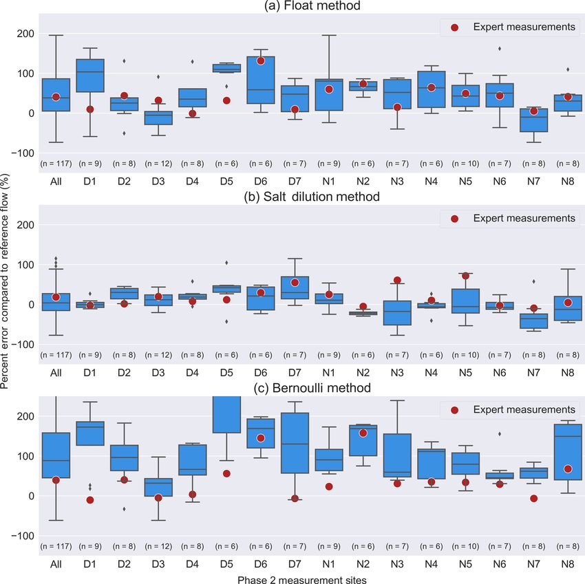
1048                    J. C. Davids et al.: Citizen science flow – an assessment of simple streamflow measurement methods

Table 1. Summary of simple streamflow measurement methods considered for further evaluation. Integer ranks of 1, 2, or 3 for inapplicability
in Nepal (especially for smaller headwater catchments); cost; required training; and complexity were given to each method, with 1 being
most favorable and 3 being least favorable. The three methods with the lowest rank were selected for further evaluation. Smartphones are not
included in equipment needs because it was assumed that citizen scientists would provide these themselves. EC: electrical conductivity.

 No.   Method           Brief description                 Equipment needs    Inapplicability   Cost   Required    Complexity   Total rank   Selected for
                                                                                   in Nepal            training                 (4 to 12)   evaluation
                                                                                                                                            (yes/no)
 1     Bernoulli        Velocity-area method. Thin        Measuring scale                 1      1           2            1            5    yes
                        flat plate (e.g., measuring
                        scale) used to measure veloc-
                        ity head. Repeated at multiple
                        stations.
 2     Current meter    Velocity-area method. Current     Current meter,                  2      3           3            2           10    no
                        meter (e.g., bucket wheel, pro-   measuring scale
                        peller, acoustic) used to
                        measure velocity. Repeated at
                        multiple stations.
 3     Deflection rod   Velocity-area method. Shaped      Deflection rod,                 3      2           2            2            9    no
                        vanes projecting into the flow    measuring scale
                        along with a method to mea-
                        sure deflection and thereby
                        computing velocity. Repeated
                        at multiple stations.
 4     Float            Velocity-area method. Time        Measuring scale,                2      1           2            1            6    yes
                        for floating object to travel     timer
                        known distance used to deter-
                        mine water velocity at
                        multiple stations.
 5     Manning–         Slope area method. Slope of       Auto level (or                  2      2           2            3            9    no
       Strickler        the water surface elevation       water level),
                        combined with estimates of        measuring scale
                        channel roughness and chan-
                        nel geometry to determine
                        flow using the Manning–
                        Strickler equation.
 6     Pitot tube       Velocity-area method. Pitot       Pitot tube,                     2      2           2            2            8    no
                        tube used to measure velocity.    measuring scale
                        Repeated at multiple stations.
 7     Salt dilution    Constant rate of known con-       EC meter, mixing                1      2           3            3            9    no
       (constant-rate   centration of salt injected       containers
       injection)       into stream. Background
                        and steady-state electrical
                        conductivity values measured
                        after full mixing. Flow is
                        proportional to rate of salt
                        injection and change in EC.
 8     Salt dilution    Known volume and concentra-       EC meter, mixing                1      2           2            2            7    yes
       (slug)           tion of salt injected as a        containers
                        single slug. EC of break-
                        through curve measured. Flow
                        is proportional to integration
                        of breakthrough curve and vol-
                        ume of tracer introduced.

  Float method streamflow measurements involve the fol-                          3. For each subsection, measure and record the following.
lowing steps.
                                                                                       a. The depth in the middle of the subsection.
  1. Select stream reach with straight and uniform flow.                               b. The width of the subsection.
                                                                                       c. The time it takes a floating object to move a known
  2. Divide cross section into several subsections (n, typi-                              distance downstream (typically 1 or 2 m) in the
     cally between 5 and 20).                                                             middle of the subsection.

Hydrol. Earth Syst. Sci., 23, 1045–1065, 2019                                                   www.hydrol-earth-syst-sci.net/23/1045/2019/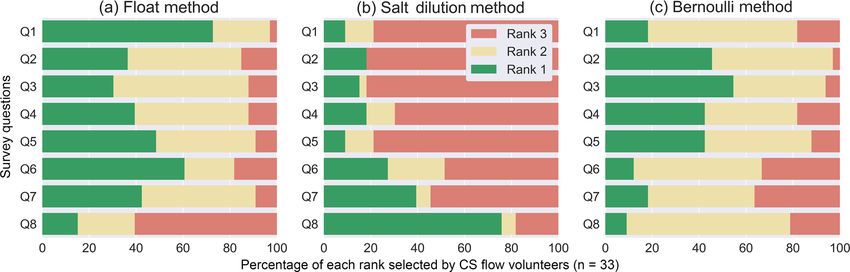
J. C. Davids et al.: Citizen science flow – an assessment of simple streamflow measurement methods                            1049

 4. Solve for streamflow (Q) with Eq. (1).                            Salt dilution method streamflow measurements involve the
                                                                   following steps.
Distances of 1 or 2 m were necessary to measure surface ve-
locity for each subsection since it was unlikely that a float       1. Select stream reach with turbulence to facilitate vertical
would stay in a single subsection for 10 or 20 m. These                and horizontal mixing.
shorter distances ensured that surface velocity measurements
were representative of their respective subsections and asso-       2. Determine upstream point for introducing the salt solu-
ciated areas. One benefit of this approach was that the mea-           tion and a downstream point for measuring EC.
sured surface velocities were cross-sectional-area weighted.
                                                                           – A rule of thumb in the literature is to separate these
This area weighting was more important as surface velocity
                                                                             locations roughly 25 stream widths apart (Day,
differences between the center and the sides of the channel
                                                                             1977; Butterworth et al., 2000; Moore, 2005).
increased. Since these velocity differences vary from site to
site, using a single float with a single coefficient (e.g., 0.8)    3. Estimate flow either by performing a “simplified float
would have ignored these differences among sites.                      measurement” (i.e., only a few subsections) or by visu-
                                                                       ally estimating width, average depth, and average veloc-
2.2.2   Salt dilution method
                                                                       ity.
There are two basic types of salt dilution flow measurements:       4. Prepare salt solution based on the following guidelines
slug (previously known as instantaneous) and continuous rate           (approximate average of dosage recommendations from
(Moore, 2004a). Salt dilution measurements are based on the            previous studies cited by Moore, 2005).
principle of the conservation of mass. In the case of the slug
method, a single known volume of high-concentration salt                   a. 10 000 mL of stream water for every 1 m3 s−1 of es-
solution is introduced to a stream and the electrical conduc-                 timated streamflow.
tivity (EC) is measured over time at a location sufficiently               b. 1667 g of salt for every 1 m3 s−1 of estimated
downstream to allow good mixing (Moore, 2005). An ap-                         streamflow.
proximation of the integral of EC as a function of time is
combined with the volume of tracer and a calibration con-                  c. Thoroughly mix salt and water until all salt is dis-
stant (Eq. 2) to determine discharge. In contrast, the contin-                solved.
uous rate salt dilution method involves introducing a known                d. Following these guidelines, ensure a homogenous
flow rate of salt solution into a stream (Moore, 2004b). Slug                 salt solution with 1 to 6 salt to water ratio by mass.
method salt dilution measurements are broadly applicable in
streams with flows up to 10 m3 s−1 with steep gradients and         5. Establish the calibration curve relating EC values to ac-
low background EC levels (Moore, 2005). For the sake of                tual salt concentrations (Moore, 2004b) to determine the
citizen scientist repeatability, we chose to only investigate          calibration constant (k) relating changes in EC values in
the slug method, because of the added complexity of mea-               microsiemens per centimeter (µS cm−1 ) in the stream to
suring the flow rate of the salt solution for the continuous           relative concentration (RC) of introduced salt solution
rate method. Some limitations of the salt dilution method in-          (see Sect. 2.3.3 for details).
clude (1) inadequate vertical and horizontal mixing of the          6. Dump salt solution at upstream location.
tracer in the stream, (2) trapping of the tracer in slow-moving
pools of the stream, and (3) incomplete dilution of salt within     7. Measure EC at downstream location during salinity
the stream water prior to injection. The first two limitations         breakthrough until values return to background EC.
can be addressed with proper site selection (i.e., well-mixed
reach with little slow-moving bank storage), while incom-                  – Record a video of the EC meter screen at the down-
plete dilution can be avoided by proper training of the per-                 stream location and later digitize the values using
sonnel performing the measurement.                                           the time from the video and the EC values from the
   Streamflow (Q; L s−1 ) is solved for using Eq. (2) (Rantz,                meter.
1982; Moore, 2005):                                                 8. Solve for streamflow (Q) with Eq. (2).
             V
Q = Pn                    ,                                 (2)    2.2.3    Bernoulli run-up method
   k i=1 (σ (t) − σBG )1t
where V is the total volume of tracer introduced into the          Like the float method, Bernoulli run-up (or Bernoulli) is
stream (L), k is the calibration constant in centimeters per       based on the velocity-area principle. The basic principle is
microsiemens (cm µS−1 ), n is the number of measurements           that run-up on a flat plate inserted perpendicular to flow is
taken during the breakthrough curve (unitless), σ (t) is the EC    proportional to velocity based on the solution to Bernoulli’s
at time t (µS cm−1 ), σBG is the background EC (µS cm−1 ),         equation. Bernoulli run-up is also referred to as the “velocity
and 1t is the change in time between EC measurements (s).          head rod” by Church and Kellerhals (1970), Carufel (1980),

www.hydrol-earth-syst-sci.net/23/1045/2019/                                      Hydrol. Earth Syst. Sci., 23, 1045–1065, 2019
1050 J. C. Davids et al.: Citizen science flow – an assessment of simple streamflow measurement methods
and Fonstad et al. (2005) and is similar to the “weir stick” stream types. Streamflows ranged from 0.4 to 1804 L s−1 .
discussed by USBR (2001). The velocity measurement the- Stream widths and average depths ranged from 0.1 to 6.0 m
ory of Bernoulli is similar to using a pitot tube (Almeida and and from 0.0040 to 0.97 m, respectively. Streambed materials
de Souza, 2017), without the associated challenges of (1) us- ranged from cobles, gravels, and sands in the upper portions
ing and transporting potentially bulky and fragile equipment of the watershed to sands, silts, and sometimes man-made
and (2) clogging from sediment or trash (WMO, 2010). How- concrete streambeds and side retaining walls in the lower
ever, the accuracy and precision of the Bernoulli method ve- portions. During pre-monsoon, sediment loads were gener-
locity head measurements are likely lower than pitot mea- ally low, while during post-monsoon increased water veloc-
surements. Total streamflow (Q; L s−1 ) is calculated with ities led to increased sediment loads (both suspended and
Eq. (3): bed). Slopes (based on phase 2 data) ranged from 0.020 to
Xn 0.148 m m−1 . Additional details about the measurement sites
Q = 1000 · V · d1i · wi ,
i=1 Bi
(3) are provided in Tables 4 and 5. Since roughly 80 % of Nepal’s
precipitation occurs during the summer monsoon (Nayava,
where 1000 is a conversion factor from m3 s−1 to L s−1 , VBi 1974), pre- and post-monsoon represent periods of relatively
is the velocity from Bernoulli run-up (m s−1 ), d1i is the depth low and high streamflows, respectively. Therefore, we con-
(m), and wi is the width (m) of each subsection (i = 1 to sistently use pre-monsoon and post-monsoon to refer to the
n). Area for each subsection is the product of the width and general seasons that phase 1, 2, and 3 activities were per-
the depth in the middle of each subsection. Velocity for each formed in.
subsection (VBi ) was determined by measuring the run-up or
change in water level on a thin meter stick (or “flat plate”;
dimensions used in this study: 1 m long by 34 mm wide by 2.3.2 Reference flows
1.5 mm thick) from when the flat plate was inserted parallel
and then perpendicular to the direction of flow. The parallel
depth measurement represents the static head, while the per- To evaluate different simple citizen science flow measure-
pendicular represents the total head. Velocity (VBi ; m s−1 ) is ment methods, reference (or actual) flows for each site were
calculated from Bernoulli’s principle with Eq. (4): needed. We used a SonTek FlowTracker acoustic Doppler ve-
p locimeter (ADV) to determine reference flows. The United
VBi = 2g · (d2i − d1i ), (4) States Geological Survey (USGS) midsection method was
used, following guidelines from USGS Water Supply Pa-
where g is the gravitational constant (m s−2 ), and d2i and d1i
per 2175 (Rantz, 1982), along with instrument-specific rec-
are the water depths (m) when the flat plate was perpendicu-
ommendations from SonTek’s FlowTracker manual (SonTek,
lar and parallel to the direction of flow, respectively.
2009). Stream depths were shallow enough that a single ver-
Bernoulli method streamflow measurements involve the
tical 0.6 depth velocity measurement (i.e., 40 % up from the
following steps.
channel bottom) was used to measure average velocity for
1. Select constricted stream section with elevated velocity each subsection (Rantz, 1982). While there is uncertainty
to increase the difference between d1i and d2i . in using the 0.6 depth as representative of average velocity,
Rantz (1982) states that “actual observation and mathemati-
2. Divide cross section into several subsections (n, typi- cal theory have shown that the 0.6 depth method gives reli-
cally between 5 and 20). able results” for depths less than 0.76 m; multipoint methods
are not recommended for depths less than 0.76 m, so this is
3. For each subsection, measure and record the following.
the recommended USGS approach. Depending on the total
a. The depth with a flat plate held perpendicular to width of the channel, the number of subsections ranged from
flow (d2i or the run-up depth). 8 to 30. The FlowTracker ADV has a stated velocity mea-
surement accuracy of within 1 % (SonTek, 2009). Based on
b. The depth with a flat plate held parallel to flow (d1i
an ISO discharge uncertainty calculation within the SonTek
or the actual water depth).
FlowTracker software, the uncertainties in reference flows
c. The width of the subsection. for phases 1 and 2 ranged from 2.5 % to 8.2 %, with a mean
of 4.2 %. Based on the literature (Rantz, 1982; Harmel, 2006;
4. Solve for streamflow (Q) with Eqs. (3) and (4).
Herschy, 2009), these uncertainties in reference flows are to-
2.3 General items wards the lower end of the expected range for field mea-
surements of streamflow. Therefore, we do not think that any
2.3.1 Types of streams evaluated systematic biases or uncertainties in our data change the re-
sults of this paper. A compilation of the measurement reports
Streams evaluated during this investigation (phases 1, 2, and generated by the FlowTracker ADV, including summaries of
3) were a mixture of pool and riffle, pool and drop, and run measurement uncertainty, is included in the Supplement.
Hydrol. Earth Syst. Sci., 23, 1045–1065, 2019 www.hydrol-earth-syst-sci.net/23/1045/2019/J. C. Davids et al.: Citizen science flow – an assessment of simple streamflow measurement methods 1051
2.3.3 Salt dilution calibration coefficient (k)
Our experience was that the most complicated portion of a
salt dilution measurement was performing the dilution test
to determine the calibration coefficient k. The calibration
coefficient k relates changes in EC values in microsiemens
per centimeter (µS cm−1 ) in the stream to relative concentra-
tions of introduced salt solution (RC). During phases 1 and
2, we determined k using a calibrated GHM 3431 (GHM-
Greisinger) EC meter with the procedure recommended by
Moore (2004b; additional details are included in the Supple-
ment).
Due to the challenges of measuring k in the field, espe-
cially for citizen scientists who are the ultimate target for Figure 1. Box plots of inexpensive water quality tester (HoneFor-
performing these streamflow measurements, average k val- est) errors for five different intervals (i.e., D1 to D5). The ranges
ues were used to determine salt dilution streamflows. For of EC values from reference EC measurements (determined by a
calibrated GHM 3431 (GHM-Greisinger) EC meter) are shown in
phase 1, an average k of 2.79 × 10⁻⁶ µS cm−1 µS cm−1 (n =
parentheses in µS cm−1 . Boxes show the interquartile range be-
10) was used for all 20 measurement sites (Table 4). For
tween the first and third quartiles of the dataset, while whiskers
phase 2, an average k of 2.95 × 10⁻⁶ µS cm−1 (n = 15) was extend to show minimum and maximum values of the distribution,
used for all 15 sites (Table 5). For phase 3, the phase 2 aver- except for points that are determined to be outliers (shown as dia-
age k of 2.95 × 10⁻⁶ µS cm−1 was used to calculate stream- monds), which are more than 1.5 times the interquartile range away
flows for all salt dilution measurements. The impact of using from the first or third quartiles.
average k values on salt dilution measurements is discussed
in Sect. 4.1. Moore (2005) suggests that k is a function of
(1) the ratio of salt and water in the tracer solution and (2) the 2.4 Phases of the investigation
chemical composition of the stream water. To minimize vari-
ability in k due to changes in salt concentration, a fixed ratio This investigation was carried out in three distinct phases in-
of salt to water (i.e., 1 to 6 by mass) was used to prepare cluding phase 1 – initial evaluation, phase 2 – citizen sci-
tracer solutions for all phases of this investigation. entist evaluation, and phase 3 – citizen scientist application
(Table 2).
2.3.4 Inexpensive EC meters
2.4.1 Initial evaluation (phase 1)
For phases 2 and 3, 10 inexpensive (i.e., USD 15) water qual-
ity testers (HoneForest) were used to measure EC for salt di- For phase 1 evaluation of the three simple streamflow mea-
lution measurements. To evaluate the accuracy of these me- surement methods, we performed sets of measurements at
ters, we performed a six-point comparison test with reference 20 sites within the Kathmandu Valley, Nepal (Fig. 2a and b).
EC values of 20, 107, 224, 542, 1003, and 1517 µS cm−1 , The Kathmandu Valley is a small intermontane basin roughly
as determined by a calibrated GHM 3431 (GHM-Greisinger) 25 km in diameter with a total area of 587 km2 in the central
EC meter. EC measurements were performed from low EC to region of Nepal and encompasses most of the Kathmandu,
high EC (for all six points) and were repeated three times for Bhaktapur, and Lalitpur districts. Figure 2c is a photograph
each meter. Because EC is used to compute the integral of of the typical types of relatively steep pool and drop stream
the breakthrough curve (Eq. 2), the percent difference (i.e., systems included in phase 1. Sites were chosen to represent a
error) in EC changes between the six points (i.e., five inter- typical range of stream types, slopes, and flow rates. At each
vals) from the inexpensive meters was compared to reference site, we performed float, salt dilution, and Bernoulli mea-
EC intervals (Fig. 1). Based on this analysis, the inexpensive surements, in addition to reference flow measurements with
meters had a positive median bias of roughly 5 % (ranging the FlowTracker ADV as per the descriptions in Sect. 2.2
from −14 % to 21 %) for EC value changes between 20 and and 2.3.2, respectively. All phase 1 salt dilution EC mea-
542 µS cm−1 (i.e., D1, D2, and D3). A nearly zero median surements were taken with a calibrated GHM 3431 (GHM-
bias (ranging from −5 % to 5 %) for EC value changes be- Greisinger) EC meter.
tween 542 and 1003 µS cm−1 (i.e., D4) was present. Finally, At each site, measurements were performed consecutively
there was a negative median bias of roughly −9 % (ranging and took roughly 1 to 2 h to perform, depending on the size of
from −18 % to 6 %) for EC value changes between 1003 and the stream and the resulting number of subsections for float,
1517 µS cm−1 (i.e., D5). No corrections were made to EC Bernoulli, and reference flow measurements. Measurements
measurements collected with inexpensive (HoneForest) EC were performed during steady-state conditions in the stream;
meters. if runoff-generating precipitation occurred during measure-
www.hydrol-earth-syst-sci.net/23/1045/2019/ Hydrol. Earth Syst. Sci., 23, 1045–1065, 20191052 J. C. Davids et al.: Citizen science flow – an assessment of simple streamflow measurement methods
Table 2. Brief descriptions of three data collection phases including who performed the field data collection and what period and season the
data were collected in.
No. Phase Description Performed by Period Season
1 Initial evaluation Initial evaluation of three sim- Authors March/April 2017 Pre-monsoon
ple flow measurement meth-
ods (i.e., float, salt dilution,
and Bernoulli) along with
FlowTracker ADV reference
flow measurements at 20 sites
within the Kathmandu Valley.
Reference flows ranged from
6.4 to 240 L s−1 .
2 Citizen scientist Citizen scientist evaluation of Authors for expert and refer- September 2018 Post-
evaluation three simple flow measure- ence flows plus 10 Citizen Sci- monsoon
ment methods (i.e., float, salt ence Flow groups for simple
dilution, and Bernoulli) along methods
with expert and FlowTracker
ADV reference flow measure-
ments at 15 sites within the
Kathmandu Valley. Reference
flows ranged from 4.2 to
896 L s−1 .
3 Citizen scientist Salt dilution measurements at 18 Citizen Science Flow April and September 2018 Pre- and post-
application roughly 130 sites in the 10 groups (8 from April and 10 monsoon
perennial watersheds of the from September)
Kathmandu Valley. Float mea-
surements with a small num-
ber of subsections (e.g., three
to five) performed at each site
to determine salt dosage. Ob-
served flows ranged from 0.4
to 425 L s−1 and from 1.1 to
1804 L s−1 in pre and post-
monsoon, respectively.
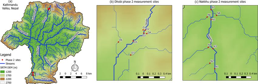
Figure 2. Map showing topography of the Kathmandu Valley from a Shuttle Radar Topography Mission (SRTM, 2000) digital elevation
model (DEM), the resulting stream network (Davids et al., 2018), and locations of phase 1 measurement sites (a). Names of the 10 historically
perennial tributaries are shown. (b) shows an enlarged view of the area where 11 of the 20 measurements were taken. (c) is a photograph of
site 11, a pool and riffle sequence flowing at roughly 100 L s−1 . Measurement sites are labeled with phase 1 site IDs.
Hydrol. Earth Syst. Sci., 23, 1045–1065, 2019 www.hydrol-earth-syst-sci.net/23/1045/2019/J. C. Davids et al.: Citizen science flow – an assessment of simple streamflow measurement methods 1053
ments at a site, the measurements were stopped and then tion of measurement reaches or the results of the stream-
repeated after streamflows stabilized at pre-event levels. As flow measurements with other groups. For the remainder
previously described, the salt dilution calibration coefficient of 18 September and all of 19 September, the 10 CS Flow
k was determined at 10 of the 20 sites. Field notes for float, groups rotated between the seven sites in the Dhobi water-
salt dilution, and Bernoulli methods were taken manually and shed. To ensure that measurements could be compared with
later digitized into a spreadsheet (included in the Supple- each other, four S4W-Nepal interns traveled between sites to
ment). Results from phase 1 are summarized in tabular form verify that CS Flow groups performed measurements on the
(Table 4). To understand relative (normalized) errors, we cal- same streams in the same general locations. All eight mea-
culated percent differences in relation to reference flow for surements on the Nakkhu watershed were performed in sim-
each method. Averages of absolute value percent differences ilar fashion on 20 September.
(absolute errors), average errors (bias), and standard devia- Using the same schedule of the CS Flow groups, the expert
tions of errors were used as metrics to compare results among group visited the same 15 sites. At each site, in addition to
methods and between phases 1 and 2. performing float, salt dilution, and Bernoulli measurements,
the expert group performed (1) reference flow measurements
2.4.2 Citizen scientist evaluation (phase 2) as per Sect. 2.3.2, (2) salt dilution calibration coefficient k
dilution measurements as per Sect. 2.3.3, and (3) an auto-
To evaluate the same three streamflow measurement meth- level survey to determine average stream slope. At each site,
ods with actual citizen scientists, we recruited 37 student vol- auto-level surveys included topographical surveys of stream
unteers from Khwopa College of Engineering in Bhaktapur, water surface elevations with a 24X Automatic Level AT-B4
Nepal, for our Citizen Science Flow (CS Flow) evaluation. A (Topcon) at five locations including 10 times and 5 times the
total of 10 CS Flow evaluation groups of either three or four stream width upstream of the reference flow measurement
members were formed. Citizen scientists were second- and site (reference site), at the reference site, and 5 and 10 times
third-year civil engineering bachelor’s degree students rang- the stream width downstream of the reference site. For each
ing in age from 21 to 25; 12 were female and 25 were male. site, stream slope was taken as the average of the four slopes
Phase 2 citizen scientist evaluations (Fig. 3) were performed computed from the five water surface elevations measured.
at seven sites in the Dhobi watershed in the north (Fig. 3b; All CS Flow and expert measurements were conducted un-
D1 to D7) and eight sites in the Nakkhu watershed in the der steady-state conditions. Based on two S4W-Nepal citi-
south (Fig. 3c; N1 to N8). Sites were chosen to represent a zen scientists’ precipitation measurements (official govern-
typical range of stream types, slopes, and flow rates found ment records are not available until the subsequent year)
within the headwater catchments of the Kathmandu Valley nearby the Dhobi sites (i.e., roughly 3 km to the west and
and to minimize travel time between locations. east), no measurable precipitation occurred during 18 and
Phase 2 started on 17 September 2018 with a 4 h theoret- 19 September. Water level measurements from a staff gauge
ical training on the float, salt dilution, and Bernoulli stream- installed at site D3 taken at the beginning and end of 18
flow measurement methods as per Sect. 2.2. The theoretical and 19 September confirmed that water levels (and therefore
training also introduced citizen scientists to Open Data Kit flows) remained steady. On 20 September, 7 mm of precipi-
(ODK; Anokwa et al., 2009), a freely available open-source tation was recorded by a S4W-Nepal citizen scientist in Tik-
software for collecting and managing data in low-resource abhairab, which is roughly 1 km north of the eight measure-
settings. ODK was used with the specific streamflow mea- ment sites in the Nakkhu watershed. Based on field obser-
surement workflow described below. vations of the expert group, rain did not start until 15:30 LT,
Based on our initial experiences and results from phase 1, and all CS Flow group measurements were completed before
we developed an ODK form to facilitate the collection of 15:30 LT. Three expert measurement sites were completed
float, salt dilution, Bernoulli, and reference streamflow mea- after 15:30 LT, but most rain was concentrated downstream
surement data. After installing ODK on an Android smart- (to the north) of these sites (i.e., N1, N2, and N3). Based on
phone and downloading the necessary form from S4W- water level measurements performed at the beginning, mid-
Nepal’s ODK Aggregate server on the Google Cloud App dle, and end of measurements at these sites, no changes in
Engine, the general workflow is included in the Supplement. water levels (and therefore flows) were observed. We also do
Training was continued on 18 September with a 2 h field not see any systematic impacts to the resulting comparison
demonstration session in the Dhobi watershed located in the data for these sites (Table 5 and Fig. 4).
north of the Kathmandu Valley. During this field training, Once ODK forms from all 15 sites were finalized and
we worked with three to four groups at a time and together submitted to the ODK Aggregate server, CS Flow and ex-
performed float, salt dilution, and Bernoulli measurements at pert groups digitized breakthrough curves (i.e., time and EC)
site D3. from EC videos in shared Google Sheets salt dilution flow
Following the field training, a Google My Map with the calculators. Digitizations for all measurements were then re-
15 sites was provided to the citizen scientists. Groups were viewed for accuracy and completeness by the authors.
strictly instructed to not discuss details regarding the selec-
www.hydrol-earth-syst-sci.net/23/1045/2019/ Hydrol. Earth Syst. Sci., 23, 1045–1065, 20191054 J. C. Davids et al.: Citizen science flow – an assessment of simple streamflow measurement methods
Figure 3. Map showing topography of the Kathmandu Valley, stream network, and locations of phase 2 measurement sites (a). Names of the
10 historically perennial tributaries are shown. (b) shows an enlarged view of the upper Dhobi watershed where phase 2 measurements D1
through D7 were performed. (c) shows an enlarged view of the middle Nakkhu watershed where phase 2 measurements N1 through N8 were
performed. Measurement sites are labeled with phase 2 site IDs.
After the completion of phase 2 field work, a Google Post-monsoon phase 3 measurements were performed by
Forms survey was completed by 33 of the phase 2 citizen the same 10 CS Flow groups that performed phase 2 citizen
scientists (Table 3). The purpose of the survey was to evalu- scientist evaluations. Therefore, additional training for these
ate citizen scientists’ perceptions of the three simple stream- groups was not necessary. Training for pre-monsoon CS
flow measurement methods. The survey questions forced par- Flow groups included a 4 h theoretical training on 15 April
ticipants to rank each method from 1 to 3. Questions were about the float and salt dilution streamflow measurement
worded so that in all cases a rank of 1 was most favorable methods as per Sect. 2.2. The theoretical training also in-
and 3 was least favorable. troduced citizen scientists to ODK Android data collection
A tabular summary of the 15 phase 2 measurement loca- application. For both pre- and post-monsoon phase 3 mea-
tions was developed (Table 5). To understand relative (nor- surements, the workflow was similar to that described in
malized) errors, we calculated percent differences in rela- Sect. 2.4.2 (see the Supplement for details), with the excep-
tion to reference flow for each method. Averages of absolute tions of (1) skipping collection of Bernoulli data and (2) only
value percent differences (absolute errors), average errors performing a simplified float measurement involving only
(bias), and standard deviations of errors were used as metrics two or three subsections in order to have a flow estimate for
to compare results among methods and between phase 1 and calculating the recommended salt dose. Training was con-
2. Box plots showing the distribution of CS Flow group mea- tinued on the afternoon of 15 April with a 2 h field demon-
surement errors along with expert measurement errors for stration session in the Hanumante watershed located in the
each method were developed (Fig. 4). To visualize the results southwestern portion of the Kathmandu Valley (Fig. 6). Dur-
of the citizen scientists’ perception survey, a stacked hori- ing this field training, we worked with four groups at a time
zontal bar plot grouped by streamflow measurement methods and together performed simplified float and Bernoulli mea-
was developed (Fig. 5). surements at two sites.
After training was completed, citizen scientists were sent
to the field to perform streamflow measurements as described
2.4.3 Citizen scientist application (phase 3) above in all 10 headwater catchments of the Kathmandu Val-
ley (Fig. 6). All phase 3 salt dilution EC breakthrough curve
From 15 to 21 April 2018 (pre-monsoon) and from 21 to measurements were performed with inexpensive (HoneFor-
25 September 2018 (post-monsoon), 25 and 37 second- and est) meters. Once ODK forms from all phase 3 measure-
third-year engineering bachelor’s degree student citizen sci- ments were finalized and submitted to the ODK Aggregate
entists, respectively, from Khwopa College of Engineering in server, CS Flow groups digitized breakthrough curves (i.e.,
Bhaktapur, Nepal, joined S4W-Nepal’s Citizen Science Flow time and EC) from EC videos in shared Google Sheets salt
campaign. Citizen scientists formed 8 pre-monsoon and 10 dilution flow calculators. Digitizations for all measurements
post-monsoon CS Flow groups of three or four people each. were then reviewed for accuracy and completeness by the au-
Ages of pre-monsoon citizen scientists ranged from 21 to 25; thors. While not included in this paper, it is important to note
7 were female and 18 were male (post-monsoon group com- that students analyzed the collected flow data and finally pre-
position is described in Sect. 2.4.2). sented oral and written summaries of their quality-controlled
Hydrol. Earth Syst. Sci., 23, 1045–1065, 2019 www.hydrol-earth-syst-sci.net/23/1045/2019/J. C. Davids et al.: Citizen science flow – an assessment of simple streamflow measurement methods 1055
Figure 4. Box plots showing distribution of CS Flow group percent errors compared to reference flows for (a) float, (b) salt dilution, and
(c) Bernoulli streamflow measurement methods. A summary of “all” measurements followed by the 15 phase 2 measurement sites (i.e., D1 to
D7 in the Dhobi watershed and N1 to N8 in the Nakkhu watershed) is shown on the horizontal axes. Percent errors for expert measurements
for each site and method are shown as red circles. The expert measurements shown for “all” are the mean of all expert measurements for
each method. Sample sizes for each method and each site are shown in parentheses above each site label. Boxes show the interquartile range
between the first and third quartiles of the dataset, while whiskers extend to show minimum and maximum values of the distribution, except
for points that are determined to be outliers (shown as diamonds), which are more than 1.5 times the interquartile range away from the first
or third quartiles. To facilitate comparison between sub-panels, vertical axes are fixed from −150 % to 250 %. In certain cases, portions of
the error distribution are outside of the fixed range (e.g., site D5 for the Bernoulli method, c).
Table 3. Summary of phase 2 survey questions and the meanings of ranks.
No. Question Rank 1 Rank 3
meaning meaning
Q1 Required training for each method Least Most
Q2 Cost of equipment for each method Least Most
Q3 Number of citizen scientists required for each method Least Most
Q4 Data-recording requirements for each method Least Most
Q5 Complexity of procedure for each method Least Most
Q6 Enjoyability of measurement method Most Least
Q7 Safety of each method Most Least
Q8 Accuracy of each method Most Least
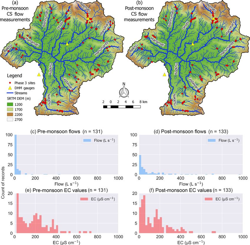
www.hydrol-earth-syst-sci.net/23/1045/2019/ Hydrol. Earth Syst. Sci., 23, 1045–1065, 20191056 J. C. Davids et al.: Citizen science flow – an assessment of simple streamflow measurement methods Figure 5. Results of the CS Flow group perception questions for (a) float, (b) salt dilution, and (c) Bernoulli methods. Questions Q1 through Q8 are shown on the vertical axis. Percentages of each rank selected by CS Flow citizen scientists (n = 33) are shown on the horizontal axis. Questions were worded so that in all cases a rank of 1 was most favorable and 3 was least favorable. Questions are as follows (also included in Table 3): Q1 – required training (rank 1 meaning least and 3 most); Q2 – cost of equipment (rank 1 meaning least and 3 most); Q3 – number of citizen scientists required (rank 1 meaning least and 3 most); Q4 – data-recording requirements (rank 1 meaning least and 3 most); Q5 – complexity of procedure (rank 1 meaning least and 3 most); Q6 – enjoyability of measurement (rank 1 meaning most and 3 least); Q7 – safety (rank 1 meaning most and 3 least); Q8 – accuracy (rank 1 meaning most and 3 least). Figure 6. CS Flow campaign measurement locations (n = 131 pre-monsoon; n = 133 post-monsoon) within the Kathmandu Valley for (a) pre- and (b) post-monsoon. Histograms show distributions of measured flows in L s−1 (c, d) and EC in µS cm−1 (e, f). Bins are set to 20 units wide for both flow and EC. Three flow measurements for the post-monsoon (d) that were above 1000 L s−1 are not shown: 1059, 1287, and 1804. Three Department of Hydrology and Meteorology (DHM) gauging stations are shown as yellow triangles. Hydrol. Earth Syst. Sci., 23, 1045–1065, 2019 www.hydrol-earth-syst-sci.net/23/1045/2019/
J. C. Davids et al.: Citizen science flow – an assessment of simple streamflow measurement methods                           1057

results to their faculty and peers at Khwopa College of Engi-     float, salt dilution, and Bernoulli methods, respectively (Ta-
neering.                                                          ble 5 and Fig. 4). Standard deviations of expert errors were
   While subsequent work will highlight the knowledge             34 %, 26 %, and 51 % for float, salt dilution, and Bernoulli
about spring and streamflows gained from these data, the          methods, respectively. Salt dilution calibration coefficients
purpose herein is more a proof of concept showing that the        (k) averaged 2.95 × 10⁻⁶ cm µS−1 and ranged from 2.62 to
salt dilution method can be successfully applied at more sites    3.42×10⁻⁶ cm µS−1 . Measurement sites in the Dhobi water-
with more people. As such, a simple map figure is used            shed were pool and drop stream types, with slopes ranging
to show the spatial distribution of measurements. The three       from 0.076 to 0.148 m m−1 . Streambeds for these sites were
streamflow gauging stations within the Kathmandu Valley           predominantly cobles, gravels, and sands. Smaller tributaries
(only one in a headwater catchment) operated by the offi-         measured in the Nakkhu watershed (N2, N4, and N6) were
cial government agency responsible for streamflow measure-        also pool and drop stream types with slopes of 0.105, 0.091,
ments (i.e., the Department of Hydrology and Meteorology          and 0.055 m m−1 , respectively. The remainder of the sites in
or DHM) are also included. Additionally, histograms of flow       the Nakkhu watershed were pool and riffle stream types with
and EC for pre- and post-monsoon are also shown. While            slopes ranging from 0.020 to 0.075 m m−1 .
measurements in pre- and post-monsoon were not all taken             Box plots of CS Flow group errors combined with ex-
in the same locations, histograms can still be used to see sea-   pert measurement errors for float (a), salt dilution (b), and
sonal changes in distributions.                                   Bernoulli (c) methods show that errors, for both expert and
                                                                  CS Flow groups, are smallest for the salt dilution method
                                                                  (Fig. 4). The number of CS Flow group measurements used
3     Results                                                     to develop individual box plots ranged from 6 to 12 for each
                                                                  site and totalled 117 for all 15 sites. Two groups measured
The following results section is organized into the same three    site D3 twice, so even though there were only 10 groups,
phases included in the methodology (Sect. 2.4): initial eval-     there were 12 measurements available for comparison for
uation (phase 1), citizen scientist evaluation (phase 2), and     this site. For the remainder of sites (except N5), problems
citizen scientist flow application (phase 3).                     with either capturing, compressing, uploading, or interpret-
                                                                  ing the video of EC used for determining salt dilution flow
3.1    Initial evaluation results (phase 1)
                                                                  limited the number of usable measurements to less than the
Reference flows evaluated in phase 1 ranged from 6.4 to           number of groups (i.e., 10). Absolute errors for CS Flow
240 L s−1 (Table 4; sorted in ascending order by reference        group measurements averaged 63 %, 28 %, and 131 %, while
flow). Elevations of measurements ranged from 1313 to             biases for all methods were positive, averaging 52 %, 7 %,
1905 m a.s.l. (meters above sea level). Salt dilution cali-       and 127 % for float, salt dilution, and Bernoulli methods, re-
bration coefficients (k) averaged 2.79 × 10⁻⁶ cm µS−1 and         spectively. Standard deviations of CS Flow group errors were
ranged from 2.57 to 3.02 × 10⁻⁶ cm µS−1 . Absolute errors         82 %, 36 %, and 225 % for float, salt dilution, and Bernoulli
with respect to reference flows averaged 23 %, 15 %, and          methods, respectively.
37 %, while biases for all methods were positive, averag-            For the float method (Fig. 4a), 13 median CS Flow group
ing 8 %, 6 %, and 26 % for float, salt dilution, and Bernoulli    errors were positive, while two sites (i.e., D3 and N7) were
methods, respectively. Standard deviations of errors were         negative. Float expert errors (i.e., red circles) were within the
29 %, 19 %, and 62 % for float, salt dilution, and Bernoulli      interquartile range (IQR; blue boxes between the first and
methods, respectively. The largest salt dilution errors oc-       third quartile) of CS Flow group errors for 10 out of 15 sites.
curred for reference flows of 21 L s−1 or less (i.e., sites 1     One float expert error and 21 CS Flow group errors were over
through 7), while float and Bernoulli errors were more evenly     100 %. Float error medians and distributions were more vari-
distributed throughout the range of observed flows. Field         able in the Dhobi watershed than the Nakkhu watershed. For
notes from Bernoulli flow measurements for two measure-           the salt dilution method (Fig. 4b), seven median CS Flow
ments (site IDs 9 and 19) were destroyed by water damage,         group errors were positive, while eight were negative. Salt
so Bernoulli flow and percent difference data were not avail-     dilution expert errors (i.e., red circles) were within the IQR
able for these sites. Detailed reports for reference flow mea-    of CS Flow group errors for 7 out of 15 sites. Zero salt di-
surements along with calculations for each simplified stream-     lution expert errors and two CS Flow group errors were over
flow measurement method are included in the Supplement.           100 %. Salt dilution error distributions were more compact
                                                                  for the Dhobi watershed compared to the Nakkhu watershed.
3.2    Citizen scientist evaluation results (phase 2)             For the Bernoulli method (Fig. 4c), all 15 median CS Flow
                                                                  group errors were positive. Bernoulli expert errors (i.e., red
Reference flows evaluated in phase 2 ranged from 4.2 to           circles) were within the IQR of CS Flow group errors for
896 L s−1 (Table 5). Absolute errors for expert measure-          3 out of 15 sites. Two Bernoulli expert errors and 50 CS
ments averaged 41 %, 21 %, and 43 %, while biases for all         Flow group errors were over 100 %. Similar to float results,
methods were positive, averaging 41 %, 19 %, and 40 % for

www.hydrol-earth-syst-sci.net/23/1045/2019/                                    Hydrol. Earth Syst. Sci., 23, 1045–1065, 2019
You can also read