Meltwater run-off from Haig Glacier, Canadian Rocky Mountains, 2002-2013
←
→
Page content transcription
If your browser does not render page correctly, please read the page content below
Hydrol. Earth Syst. Sci., 18, 5181–5200, 2014
www.hydrol-earth-syst-sci.net/18/5181/2014/
doi:10.5194/hess-18-5181-2014
© Author(s) 2014. CC Attribution 3.0 License.

Meltwater run-off from Haig Glacier, Canadian Rocky Mountains,
2002–2013
S. J. Marshall
Department of Geography, University of Calgary, 2500 University Dr NW, Calgary AB, T2N 1N4, Canada

Correspondence to: S. J. Marshall (shawn.marshall@ucalgary.ca)

Received: 14 June 2014 – Published in Hydrol. Earth Syst. Sci. Discuss.: 21 July 2014
Revised: 18 October 2014 – Accepted: 1 November 2014 – Published: 12 December 2014

Abstract. Observations of high-elevation meteorological           1   Introduction
conditions, glacier mass balance, and glacier run-off are
sparse in western Canada and the Canadian Rocky Moun-             Meltwater run-off from glacierized catchments is an inter-
tains, leading to uncertainty about the importance of glaciers    esting and poorly understood water resource. Glaciers pro-
to regional water resources. This needs to be quantified so       vide a source of interannual stability in streamflow, supple-
that the impacts of ongoing glacier recession can be eval-        menting snow melt, and rainfall (e.g. Fountain and Tangborn,
uated with respect to alpine ecology, hydroelectric opera-        1985). This is particularly significant in warm, dry years (i.e.
tions, and water resource management. In this manuscript          drought conditions) when ice melt from glaciers provides the
the seasonal evolution of glacier run-off is assessed for an      main source of surface run-off once seasonal snow is de-
alpine watershed on the continental divide in the Canadian        pleted (e.g. Hopkinson and Young, 1998). At the same time,
Rocky Mountains. The study area is a headwaters catchment         glacier run-off presents an unreliable future due to glacier re-
of the Bow River, which flows eastward to provide an impor-       cession in most of the world’s mountain regions (Meier et al.,
tant supply of water to the Canadian prairies. Meteorologi-       2007; Radić and Hock, 2011).
cal, snowpack, and surface energy balance data collected at          There is considerable uncertainty concerning the impor-
Haig Glacier from 2002 to 2013 were analysed to evaluate          tance of glacier run-off in different mountain regions of the
glacier mass balance and run-off. Annual specific discharge       world. As an example, recent literature reports glacier inputs
from snow- and ice-melt on Haig Glacier averaged 2350 mm          of 2 % (Jeelani et al., 2012) to 32 % (Immerzeel et al., 2009)
water equivalent from 2002 to 2013, with 42 % of the run-off      within the upper Indus River basin in the western Himalaya.
derived from melting of glacier ice and firn, i.e. water stored   In the Rio Santo watershed of the Cordillera Blanca, Peru,
in the glacier reservoir. This is an order of magnitude greater   Mark and Seltzer (2003) estimate glacier contributions of
than the annual specific discharge from non-glacierized parts     up to 20 % of the annual discharge, exceeding 40 % during
of the Bow River basin. From 2002 to 2013, meltwater de-          the dry season. Based on historical streamflow analyses and
rived from the glacier storage was equivalent to 5–6 % of the     hydrological modelling in the Cordillera Blanca, Baraer et
flow of the Bow River in Calgary in late summer and 2–3 %         al. (2012) report even larger glacier contributions in highly
of annual discharge. The basin is typical of most glacier-fed     glacierized watersheds: up to 30 and 60 % of annual and dry-
mountain rivers, where the modest and declining extent of         season flows respectively. In the Canadian Rocky Mountains,
glacierized area in the catchment limits the glacier contribu-    hydrological modelling indicates glacier meltwater contribu-
tion to annual run-off.                                           tions of up to 80 % of July to September (JAS) flows, de-
                                                                  pending on the extent of glacier cover in a basin (Comeau et
                                                                  al., 2009).
                                                                     Different studies cannot be compared, as the extent of
                                                                  glacier run-off depends on the time of year and the propor-
                                                                  tion of upstream glacier cover. Close to the glacier source
                                                                  (i.e. for low-order alpine streams draining glacierized val-

Published by Copernicus Publications on behalf of the European Geosciences Union.
5182                                                                      S. J. Marshall: Meltwater run-off from Haig Glacier

leys), glacial inputs approach 100 % in late summer or in              Source waters in the Rocky Mountains need to be better
the dry season. Further downstream, distributed rainfall and        understood and quantified for water resource management
snowmelt inputs accrue, often filtered through the groundwa-        in the basin, particularly in light of increasing population
ter system such that glacier inputs diminish in importance.         stress combined with the risk of declining summer flows in
Glacier run-off also varies over the course of the year, inter-     a warmer climate (Schindler and Donahue, 2006). Based on
annually, and over longer periods (i.e. decades) as a result of     relatively simple models, glacier storage inputs (ice and firn
changing glacier area, further limiting comparison between          melt) for the period 2000–2009 have been estimated to con-
studies.                                                            stitute about 2 and 6 % of annual and JAS flow of the Bow
    Confusion also arises from ambiguous terminology:               River in Calgary (Comeau et al., 2009; Marshall et al., 2011;
glacier run-off sometimes refers to meltwater derived from          Bash and Marshall, 2014).
glacier ice and sometimes to all water that drains off a glacier,      Glacial inputs are therefore relatively unimportant in the
including both rainfall and meltwater derived from the sea-         downstream water budget for the basin relative to contri-
sonal snowpack (e.g. Comeau et al., 2009; Nolin et al., 2010).      butions from rainfall and the seasonal mountain snowpack.
The distinction is important because the seasonal snowpack          They are likely to be in decline, however, given persistently
on glaciers is “renewable” – it will persist (although in al-       negative glacier mass balance in the region over the last four
tered form) in the absence of glacier cover. In contrast,           decades and associated reductions in glacier area (Demuth et
glacier ice and firn serve as water reservoirs that are avail-      al., 2008; Bolch et al., 2010). This may impact on the avail-
able as a result of accumulation of snowfall over decades to        able water supply in late summer of drought years, when
centuries. This storage is being depleted in recent decades,        flows may not be adequate to meet high municipal, agri-
which eventually leads to declines in streamflow (Moore et          cultural, and in-stream ecological water demands. Moreover,
al., 2009; Baraer et al., 2012). Glaciers are also intrinsically    glacier run-off during warm, dry summers can be significant
renewable, but sustained multi-decadal cooling is needed to         in the Bow River (Hopkinson and Young, 1998), when de-
build up the glacier reservoir, i.e. something akin to the Lit-     mand is high and inputs from rainfall and seasonal snow are
tle Ice Age. In that sense, glaciers are similar to groundwater     scarce. Glacier run-off has also been reported to be important
aquifers; depleted aquifers can recover, but not necessarily on     in glacier-fed basins with limited glacier extent in the Euro-
time scales of relevance to societal water resource demands         pean Alps – e.g. more than 20 % of August flow of the lower
(Radic and Hock, 2014).                                             Rhone and Po Rivers (Huss et al., 2011).
    The importance of glaciers to surface run-off derived from         The analysis presented here contributes observationally
the Canadian Rocky Mountains is also unclear. Various es-           based estimates of glacial run-off, which can be used to im-
timates of glacial run-off are available for the region, based      prove modelling efforts, to understand long-term discharge
largely on modelling studies and glacier mass balance mea-          trends in glacially fed rivers (Rood et al., 2005; Schindler
surements at Peyto Glacier (Hopkinson and Young, 1998;              and Donahue, 2006), and to inform regional water resource
Comeau et al., 2009; Marshall et al., 2011), but there are          management strategies. Sections 2 and 3 provide further de-
little direct data concerning glacier inputs to streamflow for      tails on the field site and glaciometeorological observations
the many significant rivers that drain east, west, and north        for the period 2002–2013, which are used to force a dis-
from the continental divide. This manuscript presents ob-           tributed energy balance and melt model for Haig Glacier.
servations and modelling of glacier run-off from a 12-year          Section 4 summarises the meteorological regime and pro-
study on Haig Glacier in the Canadian Rocky Mountains               vides estimates of glacier mass balance and meltwater run-
with the following objectives: (i) quantification of daily and      off from the site, and Sects. 5 and 6 discuss the main hydro-
seasonal meltwater discharge from the glacier, (ii) separa-         logical results and implications.
tion of run-off derived from the seasonal snowpack and that
derived from the glacier ice reservoir, and (iii) evaluation
of glaciers as landscape elements or hydrological “response         2     Study site and instrumentation
units” within the broader scale of watersheds in the Canadian
Rocky Mountains.                                                    2.1    Regional setting
    Haig Glacier is one of several glacierized headwaters
catchments that feed the Bow River, which drains eastward           Glaciological and meteorological studies were established at
into the Canadian prairies. The Bow River is a modest but im-       Haig Glacier in the Canadian Rocky Mountains in August
portant drainage system that serves several population cen-         2000. Haig Glacier (50◦ 430 N, 115◦ 180 W) is the largest out-
tres in southern Alberta, with a mean annual naturalised flow       let of a 3.3 km2 ice field that straddles the North American
of 88 m3 s−1 (specific discharge of 350 mm y−1 ) in Calgary         continental divide. The glacier flows to the southeast into the
from 1972 to 2001 (Alberta Environment, 2004). The Bow              province of Alberta with a central flow line length of 2.7 km
River is heavily subscribed for agricultural and municipal          (Fig. 1). Elevations on the glacier range from 2435 to 2960 m
water demands, and water withdrawal allocations from the            with a median elevation of 2662 m. There is straightforward
river were frozen in 2006.                                          access on foot or by ski, enabling year-round study of glacio-

Hydrol. Earth Syst. Sci., 18, 5181–5200, 2014                                     www.hydrol-earth-syst-sci.net/18/5181/2014/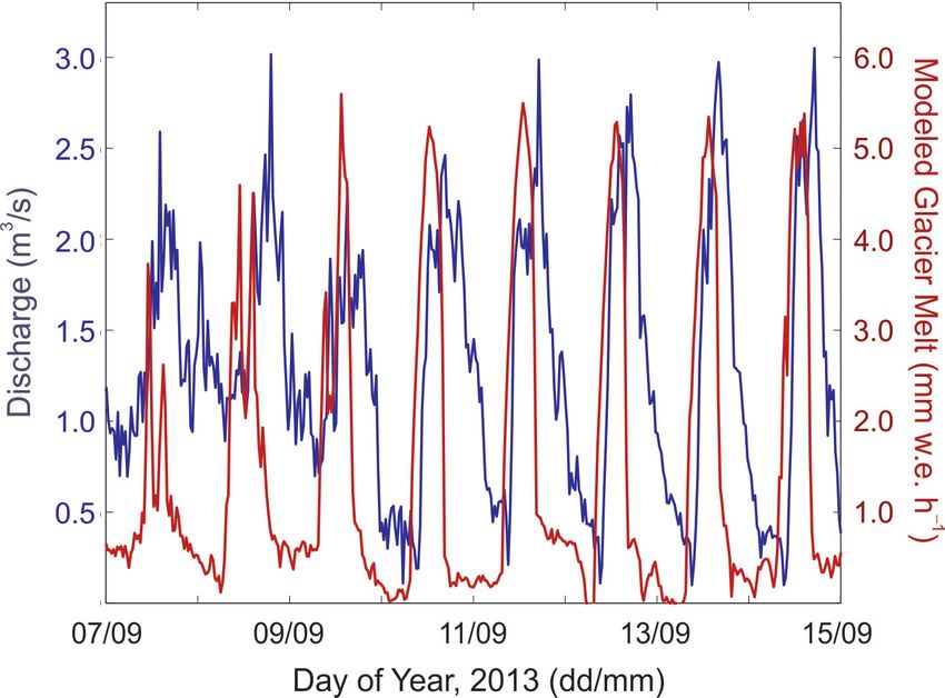
S. J. Marshall: Meltwater run-off from Haig Glacier                                                                                          5183
                                                        b

                                                                                   initial condition. Winter snowpack data used to initiate the
                                                                                   model are based on annual snow surveys typically carried
        French Pass
                                                                                   out in the second week of May. Snow depth and density
                                                                                   measurements are available from a transect of 33 sites along
                                                                                   the glacier centre line (Fig. 1), with the sites revisited each
                                              GAWS              a                  spring. Snow pits were dug to the glacier surface at four sites,
                            T/h sensor                      b                      with density measurements at 10 cm intervals, and snow
                            mb transect
                                                                                   depths were attained by probing. Sites along the transect have
              500 m                              mb10                              an average horizontal spacing of 80 m, with finer sampling on
                                                                mb02
                                                                                   the lower glacier where observed spatial variability is higher.
                                                                                      Snow survey data are available for the centre-line transect
                            20 km                                                  for 9 years from 2002 to 2013. For years without data, the
                                                                       FFAWS
      Banff                          Calgary                                        mean snow distribution for the study period was assumed.
                Bow River                                                 Stream
                                                                                   Snowpack variability with elevation, bw (z), was fit with a
                                                                          Gauge    polynomial function (Adhikari and Marshall, 2013). This
             Haig Glacier
                                                                                   function forms the basis for an estimation of the distributed
                                          b
                                                                                   snow depths and snow-water equivalence (SWE), bw (x, y).
                                                                                   This treatment neglects lateral (cross-glacier) variability in
Figure 1. Haig Glacier, Canadian Rocky Mountains, indicating the
                                                                                   the snowpack, introducing uncertainty in glacier-wide SWE
location of the automatic weather stations (GAWS, FFAWS), ad-
ditional snow pit sites (mb02, mb10, and French Pass), the mass
                                                                                   estimates. To assess the error associated with cross-glacier
balance transect (red/blue circles), the Veriteq T / h stations, and the           variation in snow depths, lateral snow-probing transects were
forefield stream gauge. Inset (a) shows the location of the study site,            carried out at three elevation bands from 2002 to 2004.
and inset (b) provides a regional perspective.
                                                                                   2.3   Meteorological instrumentation

logical, meteorological, and hydrological conditions (Shea et                      A Campbell Scientific automatic weather station (AWS) was
al., 2005; Adhikari and Marshall, 2013).                                           set up on the glacier in the summer of 2001 (GAWS) and an
   The eastern slopes of the Canadian Rocky Mountains are                          additional AWS was installed in the glacier forefield in 2002
in a continental climate with mild summers and cold win-                           (FFAWS). The weather stations are located at elevations of
ters. However, snow accumulation along the continental di-                         2665 and 2340 m respectively and are 2.1 km apart (Fig. 1).
vide is heavily influenced by moist Pacific air masses. Per-                       AWS instrumentation is detailed in Table 1. Station locations
sistent westerly flow combines with orographic uplift on the                       were stable over the study, but instruments were swapped
western flanks of the Rocky Mountains, giving frequent win-                        out on occasion for replacement or calibration. From 2001
ter precipitation events associated with storm tracks along the                    to 2008, the glacier AWS was drilled into the glacier and was
polar front (Sinclair and Marshall, 2009). This combination                        raised or lowered through additional main-mast poles dur-
of mixed continental and maritime influences gives exten-                          ing routine maintenance every few months to keep pace with
sive glaciation along the continental divide in the Canadian                       snow accumulation and melt. After 2008 the glacier AWS
Rockies, with glaciers at elevations from 2200 to 3500 m on                        was installed on a tripod. The station blew over in winter
the eastern slopes.                                                                2012–2013 and was damaged beyond recovery due to snow
   The snow accumulation season in the Canadian Rockies                            burial and subsequent drowning during snowmelt in summer
extends from October to May, though snowfall occurs in all                         2013; the last data download from the site was September
months. The summer melt season runs from May through                               2012.
September. Winter snow accumulation totals from 2002 to                               There are 2520 complete days (6.9 years) of observations
2013 averaged 1700 mm water equivalent (w.e.) at the con-                          from the GAWS from 2002 to 2012, of which 909 days are
tinental divide location at the head of Haig Glacier (results                      from June to August (JJA). This represents 90 % coverage
presented below). For comparison, October to May precipi-                          for the summer months (9.9 summers). Data are more com-
tation in Calgary, situated about 100 km east of the field site,                   plete from the FFAWS, with 3937 complete days of data
averaged 176 mm from 2002 to 2013 (Environment Canada,                             (10.8 years) and 1004 days in JJA (10.9 summers) from 2002
2014), roughly 10 % of the precipitation received at the con-                      to 2013. The glacier was visited year-round to service the
tinental divide.                                                                   weather stations with a total of 67 visits from 2000 to 2013.
                                                                                   The weather stations nevertheless failed on occasion due to
2.2    Winter mass balance                                                         power loss, snow burial, storm damage, excessive leaning,
                                                                                   and, on two occasions, blow-down. Snow burial was prob-
This study focuses on summer melt modelling at Haig                                lematic on the glacier in late winter, and in some years ob-
Glacier, with the winter snowpack taken as an “input” or                           servations at the glacier site were restricted to the summer.

www.hydrol-earth-syst-sci.net/18/5181/2014/                                                     Hydrol. Earth Syst. Sci., 18, 5181–5200, 2014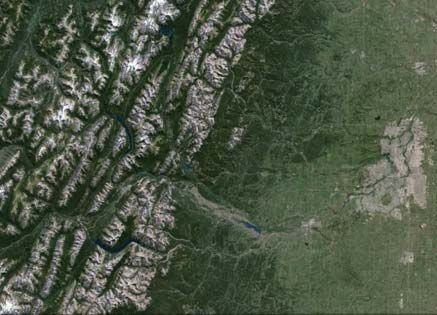
5184                                                                         S. J. Marshall: Meltwater run-off from Haig Glacier

Table 1. Instrumentation at the glacier (G) and forefield (FF) AWS sites. Meteorological fields are measured each 10 s, with 30 min averages
archived to the data loggers. Campbell Scientific data loggers are used at each site with a transition from CR10X to CR1000 loggers in
summer 2007. Radiometers are both upward and downward looking.

                        Field                   Instrument                            Comments
                        Temperature             HMP45-C
                        Relative humidity       HMP45-C
                        Wind speed/direction    RM Young 05103
                        Short wave radiation    Kipp and Zonen CM6B (FFAWS)           spectral range 0.35–2.50 µm
                                                Kipp and Zonen CNR1 (GAWS)            spectral range 0.305–2.80 µm
                        Long wave radiation     Kipp and Zonen CNR1 (GAWS)            spectral range 5–50 µm
                        Snow surface height     SR50 ultrasonic depth ranger
                        Barometric pressure     RM Young 61250V

This gives numerous data gaps at the GAWS, but there are                2002, 2003, 2013, and 2014 at a site about 900 m from the
sufficient data to examine year-round meteorological condi-             glacier terminus (Fig. 1).
tions.                                                                     The stream-gauging site and general hydrometeorological
   Additional temperature–humidity (T − h) sensors, man-                relationships are described in Shea et al. (2005). In sum-
ufactured by Veriteq Instruments Inc., were installed year-             mer 2013, continuous pressure measurements in Haig Stream
round on the glacier and were raised or lowered on site visits          were conducted from late July until late September using
in an effort to maintain a minimum measurement height of                a LevelTroll 2000. To establish a stream rating curve, dis-
more than 50 cm above the glacier surface. Sensors were en-             charge measurements were made using the velocity profile
closed in radiation shields. These sites were mainly used to            method on three different visits from July through Septem-
measure spatial temperature variability on the glacier, par-            ber, including bihourly measurements over a diurnal cycle to
ticularly near-surface temperature lapse rates. The Veriteq             capture high and low flows.
T −h transect was visited one to two times per year to down-               The run-off data are limited but provide insights into
load data and reset the loggers. Data were recorded at 30               the nature and time scale of meltwater drainage from Haig
or 60 min intervals and represent snapshots rather than aver-           Glacier. Shea et al. (2005) report delays in run-off of approx-
age conditions. During winter visits, sensors on the glacier            imately 3 h from peak glacier melt rates to peak discharge at
were raised up through additional poles in order to remain              Haig Stream during the late summer (July through Septem-
above the snow, but winter burial occurred on numerous oc-              ber). Delays are longer in May and June when the glacier is
casions, particularly on the upper glacier. In addition, there          still snow covered, probably due to a combination of mech-
was occasional summer melt-out of poles that were drilled               anisms (Willis et al., 2002): (i) the supraglacial snow cover
into the glacier, resulting in toppled sensors. Erroneous in-           acts effectively as an aquifer to store meltwater and retard
strument readings from fallen or buried sensors are easily              its drainage, (ii) access to the main englacial drainage path-
detected from low temperature variability and high, constant            ways, crevasses, and moulins is limited, and (iii) the sub-
humidity (typically 100 %); all data from these periods are             glacial drainage system (tunnel network) is not established.
removed from the analysis. Field calibrations indicate an ac-           Some early summer meltwater runs off as the proglacial wa-
curacy of ±0.4 ◦ C for daily average temperatures with the              terfall awakens and Haig Stream becomes established during
Veriteq sensors.                                                        May or June each year, initially as a sub-nival drainage chan-
                                                                        nel. A portion of early summer meltwater on the glacier may
                                                                        experience delays of weeks to months.
2.4    Stream data

Meltwater from Haig Glacier drains through a combination                3   Methods
of supraglacial streams and subglacial channels. The latter
transport the bulk of the run-off due to interception of sur-           Haig Glacier meltwater estimates in this paper are reported
face drainage channels by moulins and crevasses. Meltwater              for 2002–2013, for which winter snowpack and meteorolog-
is funnelled into a waterfall in front of the glacier, and within       ical data are available from the site. Meteorological and sur-
about 500 m of the glacier terminus run-off is collected into           face energy balance regimes are characterized at the GAWS
a single, confined bedrock channel. This proglacial stream              site, and distributed energy balance and melt models are de-
flows into the Upper Kananaskis River and goes on to feed               veloped and forced using these data. This is common practice
the Kananaskis and Bow rivers in the Rocky Mountain                     in glacier melt modelling (e.g. Arnold et al., 1996; Klok and
foothills. Glacier run-off was measured in Haig Stream in               Oerlemans, 2002; Hock and Holmgren, 2005), although sim-

Hydrol. Earth Syst. Sci., 18, 5181–5200, 2014                                          www.hydrol-earth-syst-sci.net/18/5181/2014/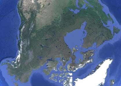
S. J. Marshall: Meltwater run-off from Haig Glacier 5185
plified temperature-index melt models are still widely used ferences in the surface energy balance as well as differences
where insufficient meteorological input data are available due to elevation.
(e.g. Huss et al., 2008; Nolin et al., 2010; Immerzeel et al., GAWS air pressure, p, is estimated from the forefield data
2013; Bash and Marshall, 2014). through the hydrostatic equation, 1p/1z = −ρa g, where 1z
Temperature-index melt models are more easily dis- is the vertical offset between the AWS sites, g is gravity,
tributed than surface energy balance models and can perform and ρa = (ρG + ρFF )/2 is the average air density between
better in the absence of local data (Hock, 2005). However, the sites. Air density is calculated from the ideal gas law at
there are numerous reasons to develop and explore more de- each site, p = ρa RT , for gas law constant R. Because this
tailed, physically based energy balance models and to resolve involves both pressure and density, air pressure and density
daily energy balance cycles, particularly as interest grows are calculated iteratively.
in modelling of glacial run-off. Diurnal processes that affect Where both GAWS and FFAWS data are unavailable,
seasonal run-off include: overnight refreezing, which delays missing meteorological data are filled using mean values for
meltwater production the following day; systematic differ- that day. For energy balance and melt modelling, diurnal cy-
ences in cloud cover through the day (e.g. cloudy conditions cles of temperature and incoming solar radiation are impor-
developing in the afternoon in summer months); diurnal de- tant. Where GAWS data are available (90 % of days for June–
velopment of the glacier boundary layer due to daytime heat- August and 86 % of days for May–September), 30 min tem-
ing; storage/delay of meltwater run-off, which can be evalu- perature and radiation data resolve the daily cycle directly.
ated from diurnal hydrographs and their seasonal evolution. Otherwise a sinusoidal temperature cycle for temperature is
These processes are not the focus of this manuscript, but the adopted, using TGs with the average measured daily temper-
model is being developed with such questions in mind, and ature range, Trd : TG (h) = TGs −Trd /2 cos(2π (t −τ )/24) for
the energy balance treatment described below will serve as a hour t ∈ (0, 24) and lag τ ∼ 4 h. For incoming solar radia-
building block for future studies. tion, the diurnal cycle is approximated using a half sinusoid
with the integrated area under the curve equal to the total
↓
3.1 Meteorological forcing data daily radiation QSd (in units of J m−2 d−1 ). Wind conditions,
specific humidity, and air pressure are assumed to be con-
stant over the day when daily fields are used to drive the melt
Meteorological data from the GAWS are used to calcu- model.
late surface energy balance at this site for the May through
September (MJJAS) melt season, and year-round daily mean 3.2 Local surface energy balance
conditions from 2002 to 2012 at the forefield and glacier
AWS sites are compiled to characterise the general meteo- Net surface energy, QN , is calculated from:
rological regime. Relations between the two sites are used ↓ ↑ ↓ ↑
to fill in missing data from the GAWS, following either QN = QS − QS + QL − QL + QG + QH + QE , (1)
βG = βFF + 1βd or βG = kd βFF , where β is the variable of ↓
interest, 1βd is the mean daily offset between the glacier and where QS is the incoming short wave radiation at the sur-
↑ ↓
forefield sites, and kd is a scaling factor used where a multi- face, QS = αs QS is the reflected short wave radiation. For
plicative relation is appropriate for mapping forefield condi- ↓ ↑
albedo αs , QL and QL are the incoming and outgoing long
tions onto the glacier. Values for 1βd and kd are calculated wave radiation, QC is the subsurface energy flux associated
from all available data for that day in the 11-year record. with heat conduction in the snow/ice, and QH and QE are
Temperature, T , is modelled through an offset, while spe- the turbulent fluxes of sensible and latent heat. Heat advec-
cific humidity, qv , wind speed, v, and incoming solar radi- tion by precipitation and run-off are assumed to be negligi-
↓
ation, QS , are scaled through factors kd . A temperature off- ble. All energy fluxes have units W m−2 . By convention, QE
set is adopted to adjust the temperature rather than a lapse- refers only to the latent heat of evaporation and sublimation.
rate correction because of the different surface energy con- QN represents the energy flux available for driving snow/ice
ditions at the two sites during the summer. After the melt- temperature changes and for latent heat of melting and re-
ing of the seasonal snowpack at the FFAWS, typically dur- freezing:
ing June, the exposed rock heats up in the sun and is not
Ts = 0 ◦ C and QN ≥ 0,
ρs Lf ṁ, (2a)
constrained to a surface temperature of 0 ◦ C as the glacier
QN = ρw Lf ṁ, Ts = 0 ◦ C and QN < 0 and water available, (2b)
surface is. Hence, summer temperature differences are much
ρs cs d ∂T , Ts < 0 ◦ C or (Ts = 0 ◦ C, QN < 0, no water). (2c)
∂t
larger than annual mean differences between the sites. Other
aspects of the energy balance regime also differ (e.g. local In general in the summer months, the glacier surface temper-
radiative and advective heating in the forefield environment). ature, Ts , is at the melting point and melt rates, ṁ (m s−1 ),
Free-air or locally determined near-surface lapse rates do not are calculated following Eq. (2a), where ρs is the surface
make sense in this situation, whereas temperature offsets cap- density (snow or ice density, with units kg m−3 ) and Lf is
ture the cooling influence of the glacier associated with dif- the latent heat of fusion (J kg−1 ). If net energy is negative, as
www.hydrol-earth-syst-sci.net/18/5181/2014/ Hydrol. Earth Syst. Sci., 18, 5181–5200, 20145186 S. J. Marshall: Meltwater run-off from Haig Glacier
is often the case at night, available surface and near-surface equivalent to the bulk transport equations for turbulent flux:
water will refreeze, following Eq. (2b) with water density
QH = CH v [T
a (z) − Ts ],
ρw = 1000 kg m−3 . The final condition in Eq. (2c) refers to (3)
QE = CE v qv (z) − qs ,
the change in internal energy of the near-surface snowpack
or glacier ice if surface temperatures are below 0 ◦ C or if where CH and CE are bulk transfer coefficients that absorb
there is an energy deficit and no meltwater is available to re- the constants and the roughness values in Eq. (3) as well as
freeze. In this case a near-surface layer of finite thickness d stability corrections.
(m) warms or cools according to the specific heat capacity, The point energy balance model is calibrated and evalu-
cs (J kg−1 ◦ C−1 ). ated at the GAWS site based on ultrasonic depth gauge melt
To evaluate the surface energy budget, the radiation terms estimates in combination with snow-pit-based snow density
are taken from direct measurements at the GAWS and QC , measurements. Local albedo measurements also assist with
QH , and QE are modelled. QC is modelled through one- this by indicating the date of transition from seasonal snow
dimensional (vertical) heat diffusion in a 50-layer, 10-m- to exposed glacier ice. Surface roughness values are tuned to
deep model of the near-surface snow or ice, forced by air achieve closure in the energy balance (e.g. Braun and Hock,
temperature at the surface–atmosphere interface and assum- 2004), adopting z0H = z0E = z0 /100 (Hock and Holmgren,
ing isothermal (0 ◦ C) glacial ice underlying the surface layer. 2005). Equation (3) is adopted in this study to permit di-
Meltwater is assumed to drain downward into the snowpack. rect consideration of roughness values, but this effectively
If the snowpack is below the melting point, meltwater re- reduces to the bulk transport equations with stability correc-
freezes and releases latent heat, which is introduced as an en- tions embedded in the roughness coefficients.
ergy source term in the relevant layer of the snowpack model.
The snow hydrology treatment is simplistic. An irreducible 3.3 Distributed model
snow water content of 4 % is assumed for the snowpack,
based on the measurements of Coléou and Lesaffre (1998), Glacier-wide run-off estimates require distributed meteoro-
and meltwater is assumed to percolate downwards into ad- logical and energy balance fields (e.g. Arnold et al., 1995;
jacent grid cells without delay. If the underlying grid cell is Klok and Oerlemans, 2002) along with characterisation of
saturated, meltwater penetrates deeper until it reaches a grid glacier surface albedo and roughness. Meteorological forc-
cell with available pore space or it reaches the snow–ice in- ing across the glacier is based on 30 min GAWS data for the
terface. The glacier ice is assumed to be impermeable, with period 1 May to 30 September, which spans the melt season.
instantaneous run-off along the glacier surface. Following the methods described in Sect. 3.1, FFAWS data
Turbulent fluxes (W m−2 ) are modelled through the stan- are used where GAWS data are unavailable. If FFAWS data
dard profile method: are also missing for a particular field, average GAWS val-
ues for that day are used as a default, based on the available
h i observations from 2002 to 2012. The glacier surface is rep-
QH = ρa cpa KH∂Ta 2 Ta (z)−Ta (z0H )
∂z = ρa cpa k v ln (z/z , resented using a digital elevation model (DEM) derived from
h 0 ) ln (z/z0H ) i (2) 2005 Aster imagery with a resolution of 1 arcsec, giving grid
∂qv 2 qv (z)−qv (z0E )
QE = ρa Ls/v KE ∂z = ρa Ls/v k v ln (z/z0 ) ln (z/z0E ) ,
cells of 22.5 m × 35.8 m.
Distributed meteorological forcing requires a number of
where z0 , z0H , and z0E are the roughness length scales for approximations regarding either homogeneity or spatial vari-
momentum, heat, and moisture fluxes (m); z is the measure- ation in meteorological and energy-balance fields. For in-
ment height for wind, temperature, and humidity (typically coming short wave radiation, slope, aspect, and elevation are
2 m); ρa is air density (kg m−3 ); cpa is the specific heat ca- taken into account through the calculation of local potential
pacity of air (J kg−1 ◦ C−1 ); Ls/v is the latent heat of sub- direct solar radiation, QSϕ (Oke, 1987):
limation or evaporation (J kg−1 ); k = 0.4 is the von Karman 2
R0
constant; K denotes the turbulent eddy diffusivities (m2 s−1 ). QSφ = I0 cos (2) ϕ p/p0 cos(Z) , (4)
R
Implicit in Eq. (3) is an assumption that the eddy diffusivi-
ties for momentum, sensible heat, and latent heat transport where I0 is the solar constant, R and R0 are the instantaneous
are equal. Equation (3) also assumes neutral stability in the and mean Earth–Sun distance, ψ is the clear-sky atmospheric
glacier boundary layer, although this can be adjusted to pa- transmissivity, p is the air pressure, and p0 is sea-level air
rameterise the effects of atmospheric stability. This reduces pressure. Angle Z is the solar zenith (i.e. sun angle), which
turbulent energy exchange due to the stable glacier boundary is a function of the time of day, day of year, and latitude, and
layer. 2 can be thought of as the effective local solar zenith angle,
Surface values are assumed to be representative of the taking into account terrain slope and aspect (Oke, 1987). For
near-surface layer – T0 (z0H ) = Ts and qv (z0E ) = qs (Ts ) – as- a horizontal surface, 2 = Z.
suming a saturated air layer at the glacier surface (e.g. Oer- For each grid cell, total daily potential direct short wave
lemans, 2000; Munro, 2004). With this treatment, Eq. (3) is radiation is calculated through integration of Eq. (5) from
Hydrol. Earth Syst. Sci., 18, 5181–5200, 2014 www.hydrol-earth-syst-sci.net/18/5181/2014/S. J. Marshall: Meltwater run-off from Haig Glacier 5187
sunrise to sunset. This is done at 10 min intervals, including Table 2. Parameters in the distributed energy balance and melt
the effects of local topographic shading based on a regional model.
DEM, i.e. examining whether a terrain obstacle is block-
Parameter Symbol Value Units
ing the direct solar beam (e.g. Arnold et al., 1996; Hock
◦C
and Holmgren, 2005). This spatial field QSϕ (x,y) is pre- Glacier temperature offset 1Td −2.8
Glacier temperature lapse rate βT −5.0 ◦ C km−1
calculated for each grid cell for each day of the year using a
clear-sky transmissivity ψ = 0.78. This value is based on cal- Specific humidity lapse rate βq −1.1 g kg−1 km−1
Summer precipitation events NP 25 ◦ C m−1
ibration of Eq. (5) at the two AWS sites for clear-sky summer Summer daily precipitation Pd 1–10 mm w.e.
days, using 2 = Z (the radiometer is mounted horizontally). Summer snow threshold TS 1.0 ◦C
Diffuse short wave radiation, Qd , also needs to be estimated, Summer fresh snow density ρpow 145 kg m−3
as there is a diffuse component to the measured radiation, Snow albedo αs 0.4–0.86
↓ Firn albedo αf 0.4
QS . I assume that mean daily Qd equals 20 % of the potential
Ice albedo αi 0.25
direct solar radiation, after Arnold et al. (1996). Assuming Snow albedo decay rate kα −0.001 (◦ C d)−1
that the mean daily diffuse fraction and clear-sky transmis- Snow/ice roughness z0 0.001 m
sivity are constant through the summer, observed daily solar Relation for εa (Eq. 5) aε 0.407
radiation on clear-sky days can then be compared with theo- [εa = aε + bε h+cε ev ] bε 0.0058
retical values of incoming radiation, QSϕ + Qd , to determine cε 0.0024 hPa−1
the effective value of ψ.
Temporal variations in incoming short wave radiation due
↑
to variable cloud cover or aerosol depth are characterized and QL ≈ 316 W m−2 . Albedo and surface temperature are
by a mean daily sky clearness index, c, calculated from the modelled in each grid cell as a function of the local snow-
ratio of measured to potential incoming solar radiation at pack evolution through the summer (see below).
↓ Turbulent fluxes are estimated at each site from Eq. (3).
the GAWS: c = QS /(QSϕ + Qd ). For clear-sky conditions,
c = 1. This is assumed to be uniform over the glacier: es- Wind speed is assumed to be spatially uniform while tem-
sentially an assumption that cloud conditions are the same perature and specific humidity are assumed to vary linearly
at all locations. Daily incoming solar radiation at point (x, with elevation on the glacier, with lapse rates βT and βq . The
↓
y) can then be estimated from QS (x, y) = c[QSϕ (x, y) + temperature lapse rate is set to −5 ◦ C km−1 based on sum-
Qd (x, y)]. mer data from the elevation transect of Veriteq temperature
Incoming long wave radiation is also taken to be uniform sensors. Note that this is a different approach from the tem-
over the glacier using the measured GAWS value. Where perature transfer function between the FFAWS and GAWS
this is unavailable, an empirical relation developed at Haig sites, as only the glacier surface environment is being consid-
Glacier is used: ered, with similar energy balance processes governing near-
surface temperature.
↓
QL = εa σ Ta4 = (aε + bε h + cε ev ) σ Ta4 , (5) In contrast, specific humidity variations in the atmosphere
are driven by larger-scale air mass, rainout, and thermody-
where σ = 5.67 × 10⁻⁸ W m−2 K−4 is the Stefan–
namic constraints, which are affected by elevation but not
Boltzmann constant, εa is the atmospheric emissivity,
necessarily the surface environment. Estimates of βq are
and Ta is the 2 m absolute air temperature. Empirical
↓ based on the mean daily gradient between the FFAWS and
formulations for QL at Haig Glacier have been exam- GAWS sites. Given local temperature and humidity, air pres-
ined as a function of numerous meteorological variables sure and density are calculated as a function of elevation from
(manuscript under review); vapour pressure and relative the hydrostatic equation and ideal gas law using FFAWS
↓
humidity provide the best predictive skill for QL , for the pressure data as described above. This gives the full energy
relation εa = aε + bε h + cε ev , relative humidity h, and balance that is needed to estimate 30 min melt totals (or if
vapour pressure ev ∈. Parameters aε , bε , and cε are locally QN < 0, refreezing or temperature changes) at all points on
calibrated and are held constant (Table 2). Equation (6) the glacier.
gives an improved representation of 30 min and daily mean Local albedo modelling is necessary to estimate absorbed
↓
values of QL at Haig Glacier relative to other empirical solar radiation, the largest term in the surface energy balance
formulations that were tested for all-sky conditions (e.g. for midlatitude glaciers (e.g. Greuell and Smeets, 2001). This
Lhomme et al., 2007; Sedlar and Hock, 2010). in turn requires an estimate of the initial snowpack based on
Outgoing short wave and long wave radiation are locally May snowpack measurements from each year. As the snow-
calculated as a function of albedo, αs , and surface tempera- pack melts, albedo declines as a result of liquid water con-
↑ ↓ ↑
ture, Ts : QS = αs QS and QL = εs σ Ts4 . Parameter εs is the tent, increasing concentration of impurities, and grain growth
thermal emissivity of the surface (∼ 0.98 for snow and ice (Cuffey and Patterson, 2010). Brock et al. (2000) showed
and ∼ 1 for water) and Ts is the absolute temperature. On a that these effects can be empirically approximated as a func-
melting glacier with a wet surface, εs → 1, Ts = 273.15 K, tion of cumulative melt or maximum daily temperatures. This
www.hydrol-earth-syst-sci.net/18/5181/2014/ Hydrol. Earth Syst. Sci., 18, 5181–5200, 20145188 S. J. Marshall: Meltwater run-off from Haig Glacier
approach is adapted here to represent snow albedo decline Table 3. Mean value ± one standard deviation of May snowpack
through the summer melt P season as a function of cumula- data based on snow pit measurements from sites at Haig Glacier,
tive positive degree days, Dd , after Hirose and Marshall 2002–2013. Glacier-wide winter mass balance, Bw , is also reported.
(2013): See Fig. 1 for snow sampling locations.
αS (t) = max [α0 − b 6Dd (t), αmin ], (6) Site z (m) depth (cm) SWE (mm) ρs (kg m−3 )
FFAWS 2340 174 ± 62 770 ± 310 400 ± 70
for fresh-snow albedo α0 , minimum snow albedo αmin , and mb02 2500 307 ± 83 1365 ± 370 445 ± 40
mb10 2590 291 ± 48 1210 ± 240 415 ± 35
coefficient b. Once seasonal snow is depleted, surface albedo GAWS 2665 304 ± 44 1230 ± 270 410 ± 50
is set to observed values for firn or glacial ice at Haig Glacier, French Pass 2750 397 ± 45 1700 ± 320 420 ± 50
αf = 0.4 and αi = 0.25. The firn zone on the glacier is speci- Glacier (Bw ) 1360 ± 230
fied based on its observed extent at elevations above 2710 m
and is assumed to be constant over the study period.
Fresh snowfall in summer is assigned an initial albedo of the snowpack pore space, and run-off may have commenced
α0 and is assumed to decline following Eq. (7) until the un- at the lowest elevations.
derlying surface is exposed again, after which albedo is set The winter snowpack as measured is an approximation
to be equal to its pre-freshened value. Summer precipitation of the true winter accumulation on the glacier, sometimes
events are modelled as random events, with the number of missing late-winter snow and sometimes missing some early
events from May through September, NP , treated as a free summer run-off. Assuming an uncertainty of 10 % associ-
variable (Hirose and Marshall, 2013). The amount of daily ated with this, combined with the independent 10 % uncer-
precipitation within these events is modelled with a uniform tainty arising from spatial variability, the overall uncertainty
random distribution varying from 1 to 10 mm. Local temper- in winter mass balance estimates can be assessed at ± 14 %.
atures dictate whether this falls as rain or snow at the glacier The melt model is initiated on 1 May for all years. While this
grid cells, with snow assumed to accumulate when T < 1 ◦ C. is not in accord with the timing of the winter snow surveys,
Parameter values in the distributed meteorological and en- there is generally little melting and run-off through May (see
ergy balance models are summarised in Table 2. The energy below); model results are not sensitive to the choice of, for
balance equations are solved to compute 30 min melt, and example, 1 May vs. 15 May. The 1 May initiation allows the
meltwater that does not refreeze is assumed to run off within snowpack ripening process to be simulated and allows the
the day. Half-hour melt totals are aggregated for each day possibility of early season melt/run-off in anomalously warm
and for all grid cells to give modelled daily run-off. springs.
4.2 Meteorological observations
4 Results
Table 4 presents mean monthly, summer, and annual meteo-
4.1 Snowpack observations rological conditions measured at the GAWS. Monthly values
are based on the mean of all available days with data for each
Winter mass balance on the glacier averaged 1360 mm w.e. month from 2002 to 2012. Figure 2 depicts the annual cycle
from 2002 to 2013 with a standard deviation of 230 mm of temperature, humidity, and wind at the two AWS sites,
w.e. (Table 3). The spatial pattern of winter snow loading as well as average daily radiation fluxes at the glacier AWS.
recurs from year to year in association with snow redistri- Values in the figure are mean daily values for the multi-year
bution from down-glacier winds interacting with the glacier data set.
topography (e.g. snow scouring on convexities, snow deposi- On average, the GAWS site is cooler, drier, and windier
tion on the lee side of the concavity at the toe of the glacier). than the glacier forefield. Mean annual wind speeds at the
Lateral snow-probing transects reveal some systematic cross- glacier and forefield AWS sites are 3.2 m s−1 and 3.0 m s−1
glacier variation in the winter snowpack, but snow depths on respectively, although the FFAWS site experiences stronger
the lateral transects are typically within 10 % of the centre summer winds. Winter (DJF) winds average 4.0 m s−1 . This
line value. More uncertain are steep, high-elevation sections is calm for a glacial environment, although there are frequent
of Haig Glacier along the north-facing valley wall (Fig. 1). wind storms at the site; peak annual 10 s wind gusts aver-
These sites cannot be sampled, so all elevations above French age 23.7 m s−1 on the glacier (85 km h−1 ) and 26.3 m s−1
Pass (2750 m) are assumed to have constant winter SWE (95 km h−1 ) at the forefield site. Katabatic winds are not
based on the value at French Pass. well developed or persistent at Haig Glacier. The low wind
In most years the snowpack is still dry and is below 0◦ C speeds and variable wind direction (not presented) indicate
during the May snow survey, with refrozen ice layers present that the glacier is primarily subject to topographically fun-
from episodic winter or spring thaws. By late May the snow- nelled synoptic-scale winds.
pack has ripened to the melting point, there is liquid water in
Hydrol. Earth Syst. Sci., 18, 5181–5200, 2014 www.hydrol-earth-syst-sci.net/18/5181/2014/S. J. Marshall: Meltwater run-off from Haig Glacier 5189
Table 4. Mean monthly weather conditions at Haig Glacier, Canadian Rocky Mountains, 2002–2012, as recorded at an automatic weather
station at 2665 m. N is the number of months with data in the 11-year record. Values are averaged over N months.
T Tmin Tmax Dd h ev qv P v
Month (◦ C) (◦ C) (◦ C) (◦ C d) (%) (mb) (g kg−1 ) (mb) (m s−1 ) αs N
Jan −11.8 −14.6 −8.9 1.6 73 1.9 1.7 738.5 4.1 0.88 5.0
Feb −11.7 −14.8 −8.5 0.3 74 2.0 1.7 739.0 3.1 0.87 5.0
Mar −10.9 −13.4 −7.9 1.2 78 2.3 2.0 738.3 3.1 0.89 5.5
Apr −5.9 −9.6 −1.6 11.2 73 3.0 2.5 741.9 2.8 0.84 7.2
May −1.6 −5.3 2.5 42.4 72 3.9 3.3 742.5 2.8 0.79 9.2
Jun 2.6 −0.4 6.2 96.3 71 5.1 4.4 747.2 2.6 0.73 10.0
Jul 6.6 3.3 10.1 217.0 62 5.9 5.0 750.8 2.8 0.59 9.8
Aug 5.8 2.6 9.4 183.8 64 5.7 5.0 750.3 2.5 0.41 9.9
Sep 1.5 −1.5 4.6 87.2 72 4.8 4.1 748.1 3.0 0.63 8.2
Oct −3.8 −6.9 −0.9 23.1 69 3.3 2.8 744.4 3.7 0.76 4.9
Nov −8.4 −11.1 −5.9 2.0 73 2.6 2.2 741.1 4.0 0.79 4.0
Dec −12.8 −15.8 −10.2 0.2 74 1.9 1.6 739.0 3.9 0.81 3.9
JJA 5.0 1.8 8.6 497.1 66 5.6 4.8 749.4 2.6 0.55 9.7
Annual −4.2 −7.3 −0.9 666.3 71 3.5 3.0 743.4 3.2 0.75 5.3
15
a 66 b
10
10
Specific Humidity (g/kg)
Temperature (°C)
55
55
00 44
-5 33
-10 22
-15
11
01/01 100
10/04 200
19/07 300
27/10 31/12 01/01 100
10/04 200
19/07 300
27/10 31/12
Day of Year (dd/mm) Day of Year (dd/mm)
c d
300
300
55
Daily Radiation (W/m )
250
2
250
Wind Speed (m/s)
44 200
200
150
150
33
100
100
2
2 50
01/01 100
10/04 200
19/07 300
27/10 31/12 01/01 100
10/04 200
19/07 300
27/10 31/12
Day of Year (dd/mm) Day of Year (dd/mm)
Figure 2. Mean daily weather at Haig Glacier, 2002–2012. Black and red lines are GAWS and FFAWS data respectively. (a) Temperature,
◦ C. The turquoise line indicates the glacier temperature derived from the FFAWS data. (b) Specific humidity, g kg−1 . (c) Wind speed, m s−1 .
(d) Radiation fields at the GAWS, W m−2 . From top to bottom: outgoing long wave (red), incoming long wave (blue), incoming short wave
(black), and outgoing short wave (orange).
Mean annual and mean summer temperatures derived from daily temperature differences between the two sites were cal-
the GAWS data are −4.2 ◦ C and +5.0 ◦ C respectively. This culated based on all available days with temperature data
compares with values of −1.3 ◦ C and +8.1 ◦ C at the FFAWS. from both AWS sites (N = 2084). The data form the basis
Temperature differences between the forefield and glacier of the temperature offset used to reconstruct temperatures on
sites are of interest because it is commonly necessary to es- the glacier when data are missing at the GAWS.
timate glacier conditions from off-glacier locations. Mean
www.hydrol-earth-syst-sci.net/18/5181/2014/ Hydrol. Earth Syst. Sci., 18, 5181–5200, 20145190 S. J. Marshall: Meltwater run-off from Haig Glacier
Temperature (°C)
1010 a a
SW Radiation (W/m )
300
300
2
55 250
00
200
200
-5-5 150
-10
-10
100
100
2 4 6 8 10 12
J F M A M J J A S O N D 50
Month
100 120 140 160 180 200 220 240 260 280 300
10/04 20/05 29/06 08/08 17/09 27/10
-4
-2
b -2 Day of Year (dd/mm)
dT/dz (°C/km)
DT (°C)
-6
-3 -3
-8
-4 -4 0.8
0.8
-10
-5
0.6
Albedo
0.6
2 4 6 8 10 12
J F M A M J J A S O N D
0.4
0.4
Month
0.2
0.2 b
Figure 3. Mean monthly temperatures at Haig Glacier, 2002–2012.
100 120 140 160 180 200 220 240 260 280 300
(a) GAWS (blue), FFAWS (red), and derived glacier means (black). 10/04 20/05 29/06 08/08 17/09 27/10
(b) Temperature differences, GAWS–FFAWS (blue, scale at right, Day of Year (dd/mm)
◦ C) and as a “lapse rate” (brown, scale at left, ◦ C km−1 ).
Figure 4. Mean daily (a) short wave radiation fluxes, W m−2 , and
(b) albedo evolution at the GAWS and FFAWS sites for the pe-
riod 1 April to 31 October 2002–2012. Black (GAWS) and red
Monthly temperature differences are plotted in Fig. 3b, ex- (FFAWS) indicate incoming radiation and purple (GAWS) and
pressed as both monthly offsets and as lapse rates. Temper- brown (FFAWS) indicate the reflected/outgoing radiation and the
ature gradients are stronger in the summer months at Haig mean daily albedo.
Glacier, with a mean of −9.3 ◦ C km−1 from July through
September. This compares with a mean annual value of
−7.1 ◦ C km−1 . This is not a true lapse rate, i.e. a measure The mean annual GAWS albedo value is 0.75 with a sum-
of the rate of cooling in the free atmosphere. Rather, tem- mer value of 0.55 and a minimum of 0.41 in August. The
perature offsets are governed by the local surface energy bal- GAWS was established near the median glacier elevation in
ance and the resultant near-surface air temperatures at each the vicinity of the equilibrium line altitude for equilibrium
site. The larger difference in summer temperatures can be at- mass balance: ELA0 , where net mass balance ba = 0. The
tributed to the strong warming of the forefield site once it glacier has not experienced a positive mass balance during
is free of seasonal snow (or, equivalently, a glacier cooling the period of study, with the snow line always advancing
effect). above the GAWS site in late summer. The transition to snow-
free conditions at the GAWS occurred from 23 July to 20
4.3 Surface energy balance August over the period of study, with a median date of 5 Au-
gust. Bare ice is exposed beyond this date until the start of
Figure 4 plots the short wave radiation budget and albedo the next accumulation season in September or October. The
evolution at the two AWS sites, illustrating this summer di- mean measured GAWS ice albedo over the full record is 0.25
vergence. Net short wave radiation is similar at the two sites with a standard deviation of 0.04. This value is applied for
through the winter until about the second week of May, af- exposed glacier ice in the glacier-wide melt modelling.
ter which time the GAWS maintains a higher albedo until Table 5 summarises the average monthly surface energy
mid-October, when the next winter sets in. Bare rock is typi- balance fluxes at the GAWS. Peak temperatures and posi-
cally exposed at the FFAWS site for about a 3-month period tive degree days are in July, but maximum net energy, QN ,
from mid-June until mid-September, with intermittent snow and meltwater production occur in August due to the lower
cover in September and early October. In wet years, snow surface albedo. Net energy over the summer (JJA) averages
persists into early July, with the FFAWS snow-free by 10 July 85 W m−2 with a peak in August at 109 W m−2 . Net radi-
in all years of the study. These dates provide a sense of the ation, Q∗, averages 63 W m−2 and makes up 74 % of the
high-elevation seasonal snow cover on non-glacierized sites available melt energy. Turbulent fluxes account for the re-
in the region. Meltwater run-off from the Canadian Rocky maining 26 % with 25 W m−2 from sensible heat transfer to
Mountains is primarily glacier-derived (a mix of snow and the glacier and a small, negative offset associated with the
ice) from mid-July through September. latent heat exchange. Sensible heat flux plays a stronger role
The albedo data also provide good constraint on the sum- at the GAWS in the month of July (34 % of available melt
mer albedo evolution and the bare-ice albedo at this site. energy). Monthly mean values of Q∗, QH , and net energy,
Hydrol. Earth Syst. Sci., 18, 5181–5200, 2014 www.hydrol-earth-syst-sci.net/18/5181/2014/S. J. Marshall: Meltwater run-off from Haig Glacier 5191
QN , are plotted in Fig. 5. To first order, QN ≈ Q ∗ +QH 2002 to 2012, ranging from 2 weeks to 3 months. The fit
through the summer melt season with monthly mean con- to the data is good (R 2 = 0.89, slope of 1.0), with an RMS
ductive and evaporative heat fluxes less than 10 W m−2 . Av- error of 170 mm w.e. The multi-week integration period aver-
erage annual melting at the GAWS is 2234 ± 375 mm w.e., ages out day-to-day differences between observations and the
of which 2034 mm (91 %) is derived in the months of June model. A plot of measured vs. modelled daily net energy bal-
through August. Summer melt ranged from 1610 to 2830 mm ance shows more scatter (Fig. 7b) with an RMS error in daily
from 2002 to 2012. Mean daily and monthly melt totals are net energy of 38 W m−2 . Scatter arises mostly due to discrep-
plotted in Fig. 5b. ancies in actual vs. modelled albedo. Although there are di-
rect albedo measurements that could be used in the model at
4.4 Distributed energy and mass balance the GAWS site, these are not available glacier-wide. For con-
sistency, the albedo is therefore modelled via Eq. (5) at the
The distributed energy balance model is run from May GAWS. Where the simulated snow-to-ice transition occurs
through September of each year based on May snowpack ini- earlier or later than in reality, this gives systematic over- or
tialisations and 30 min AWS data from 2002 to 2013. This underestimates of the net energy available for melt.
provides estimates of surface mass balance and glacier run- There are also departures associated with actual vs. mod-
off for each summer (Table 6). Glacier-wide winter snow elled summer snow events. On average, the stochastic pre-
accumulation, Bw , averaged 1360 ± 230 mm w.e. over this cipitation model predicts 9.2 ± 2.1 snow days per summer
period, with summer snowfall contributing an additional (out of 25 summer precipitation events). This is in good ac-
50 ± 14 mm w.e. This is countered by an average annual melt cord with the number of summer snow events inferred from
of 2350 ± 590 mm w.e., giving an average surface mass bal- GAWS albedo measurements. The correct timing of summer
ance of Ba = −960 ± 580 mm w.e. from 2002 to 2013. Net snow events is not captured in the stochastic summer precip-
mass balance ranged from −2300 to −340 mm w.e. over this itation model that is used, so the effects of summer snow on
period with a cumulative mass loss of 11.4 m w.e. from 2002 the snow depth and albedo are not accurately captured with
to 2013. This equates to an areally averaged glacier thinning respect to timing. For monthly or seasonal melt totals this
of 12.5 m of ice. is unlikely to be a concern, but albedo melt feedbacks could
An example of the modelled summer melt and net mass cause the stochastic model to diverge from reality. For this
balance as a function of elevation for all glacier grid cells is reason 30 realisations of the distributed model are run for
plotted in Fig. 6 for the summer of 2012. This year is rep- each summer with identical meteorological forcing, initial
resentative of mean 2002–2013 conditions at the site with snowpack, and model parameters. Values reported in Table 6
Ba = −880 mm w.e. Summer melt totals at low elevations are the averages from this ensemble of runs. The standard
on the glacier were about 3600 mm w.e., decreasing to about deviation of the net balance associated with the stochastic
1000 mm w.e. on the upper glacier (Fig. 6a). Some grid cells summer snow model is 87 mm w.e. Of this stochastic vari-
above 2650 m altitude experienced net accumulation this ability about 20 % is due to the direct mass balance impact
summer (ba > 0 in Fig. 6b), but there was no simply defined of summer snowfall and 80 % arises from the melt reduction
equilibrium line altitude (end of summer snow line eleva- due to increased albedo.
tion). This is due to differential melting as a function of topo- Glacier summer (JJA) temperature ranged from 4.1 to
graphic shading and other spatial variations in the snow ac- 6.5 ◦ C over the 12 years with a mean and standard deviation
cumulation and energy balance processes. Mass losses in the of 5.0 ± 0.8 ◦ C. Where ± values are included in the results
lower ablation zone exceeded 2000 mm w.e. Melt and mass and in the tables, it refers to ±1 standard deviation, which is
balance gradients are non-linear with elevation and are steep- reported to give a sense of the year-to-year variability. Mean
est on the upper glacier. summer albedo from 2002 to 2013 was 0.57 ± 0.04, ranging
Model results are in accord with observations of exten- from 0.48 to 0.64. The most extensive melting on record oc-
sive mass loss at the site over the study period. The snow curred in the summer of 2006, which had the highest temper-
line retreated above the glacier by the end of summer (i.e. ature, the lowest albedo, and the greatest net radiation totals,
with no seasonal snow remaining in the accumulation area) in an example of the positive feedbacks associated with exten-
2003, 2006, 2009, and 2011. Surface mass balance was mea- sive melting. On average, glacier grid cells experienced melt-
sured on the glacier from 2002 to 2005: Ba = −330, −1530, ing on 130 out of 153 days from May to September 2006,
−700, and −650 mm w.e. respectively. Observed values are compared with an average of 116 ± 8 melt days.
in reasonable accord with the model estimates with an aver- Summer 2010 offers a contrast, having the lowest number
age error of +20 mm w.e. and an average absolute error of of melt days (103), the lowest temperature, and the highest
160 mm w.e. The model underestimates the net balance for albedo. This gave limited mass loss in 2010 despite an unusu-
two of the years and overestimates it the other two. ally thin spring snowpack. Summer temperatures and melt
Figure 7a plots measured vs. modelled melt for all avail- extent are generally more influential on net mass balance
able periods with direct data (snow pits or ablation stakes) at than winter snowpack at this site. Winter mass balance is
the GAWS. Data shown are for different time periods from only weakly correlated with net balance (r = 0.16), whereas
www.hydrol-earth-syst-sci.net/18/5181/2014/ Hydrol. Earth Syst. Sci., 18, 5181–5200, 2014You can also read