Simulated or measured soil moisture: which one is adding more value to regional landslide early warning? - DORA 4RI
←
→
Page content transcription
If your browser does not render page correctly, please read the page content below
Hydrol. Earth Syst. Sci., 25, 4585–4610, 2021
https://doi.org/10.5194/hess-25-4585-2021
© Author(s) 2021. This work is distributed under
the Creative Commons Attribution 4.0 License.

Simulated or measured soil moisture: which one is adding more
value to regional landslide early warning?
Adrian Wicki1 , Per-Erik Jansson2 , Peter Lehmann3 , Christian Hauck4 , and Manfred Stähli1
1 Mountain   Hydrology and Mass Movements Research Unit, Swiss Federal Institute for Forest, Snow and Landscape Research
WSL, Zürcherstrasse 111, 8903 Birmensdorf, Switzerland
2 Department of Land and Water Resources Engineering, KTH Royal Institute of Technology, 100 44 Stockholm, Sweden
3 Institute of Terrestrial Ecosystems, ETH Zurich, Universitätstrasse 16, 8092 Zürich, Switzerland
4 Department of Geosciences, University of Fribourg, Chemin du Musée 4, 1700 Fribourg, Switzerland

Correspondence: Adrian Wicki (adrian.wicki@wsl.ch)

Received: 5 March 2021 – Discussion started: 15 March 2021
Revised: 3 August 2021 – Accepted: 3 August 2021 – Published: 26 August 2021

Abstract. The inclusion of soil wetness information in em-            gering event conditions. However, it is limited in reproducing
pirical landslide prediction models was shown to improve the          critical antecedent saturation conditions due to an inadequate
forecast goodness of regional landslide early warning sys-            representation of the long-term water storage.
tems (LEWSs). However, it is still unclear which source of
information – numerical models or in situ measurements – is
of higher value for this purpose. In this study, soil moisture
dynamics at 133 grassland sites in Switzerland were simu-             1   Introduction
lated for the period of 1981 to 2019, using a physically based
1D soil moisture transfer model. A common parameteriza-               Landslides are a major natural hazard causing fatalities and
tion set was defined for all sites, except for site-specific soil     damage in mountainous regions worldwide (Froude and
hydrological properties, and the model performance was as-            Petley, 2018). The term “landslide” includes various types
sessed at a subset of 14 sites where in situ soil moisture mea-       of mass movements spanning over different source ma-
surements were available on the same plot. A previously de-           terials (e.g. soil and rock), process dynamics (e.g. slide,
veloped statistical framework was applied to fit an empirical         flow and fall) and trigger types (e.g. water infiltration,
landslide forecast model, and receiver operating character-           earthquakes and human interaction; Hungr et al., 2014;
istic analysis (ROC) was used to assess the forecast good-            Varnes, 1978; Wieczorek, 1996). Here, we focus on rainfall-
ness. To assess the sensitivity of the landslide forecasts, the       and snowmelt-triggered shallow landslides which occur fre-
statistical framework was applied to different model parame-          quently in Switzerland (Hess et al., 2014). The landslide pro-
terizations, to various distances between simulation sites and        cess can be analysed by “cause” and “trigger” factors (Bo-
landslides and to measured soil moisture from a subset of             gaard and Greco, 2016). Factors that precondition the slope
35 sites for comparison with a measurement-based forecast             to sliding (cause factors) include the long-term weathering of
model. We found that (i) simulated soil moisture is a skil-           the slope material, the topographic disposition, the character-
ful predictor for regional landslide activity, (ii) that it is sen-   istics of the vegetation cover and the hydrological prewetting
sitive to the formulation of the upper and lower boundary             of the slope. The eventual failure of a slope along a shear
conditions, and (iii) that the information content is strongly        plane is connected to a local and short-duration decrease in
distance dependent. Compared to a measurement-based land-             shear strength (trigger factors) due to pore water pressure
slide forecast model, the model-based forecast performs bet-          increase from direct rainfall or snowmelt water infiltration
ter as the homogenization of hydrological processes, and the          or due to the indirect build-up of a perched water table or
site representation can lead to a better representation of trig-      groundwater (GW) table (Bogaard and Greco, 2016; Terlien,
                                                                      1998; Terzaghi, 1943).

Published by Copernicus Publications on behalf of the European Geosciences Union.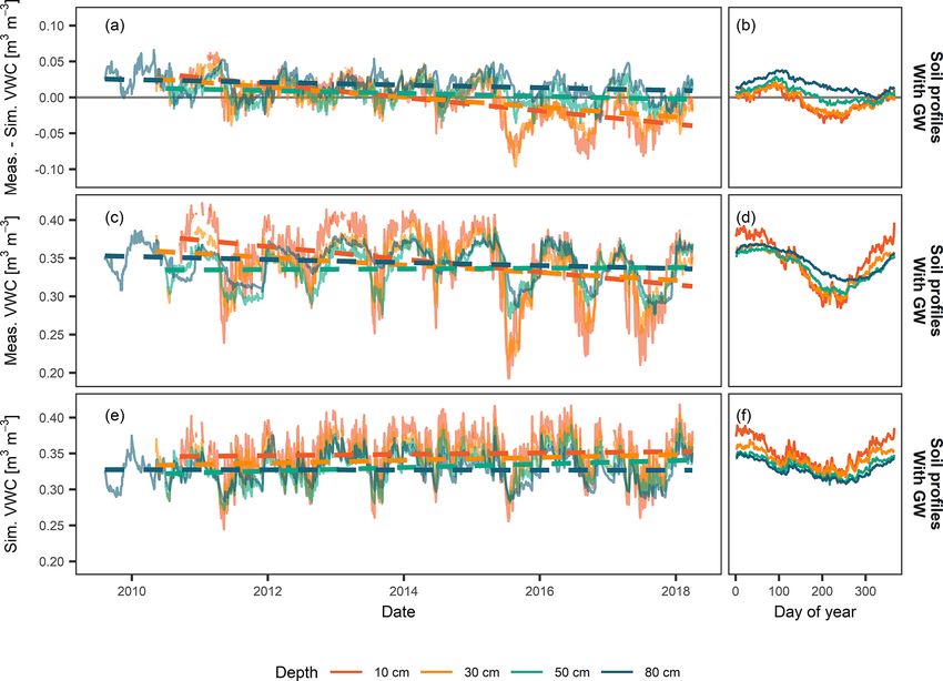
4586                                                                     A. Wicki et al.: Simulated or measured soil moisture

   Risk awareness and the corresponding response of people              Numerical models for the simulation of soil water dynam-
is a significant factor for mortality, particularly during shal-     ics may help in this regard as they provide cheap, contin-
low landslide events (Pollock and Wartman, 2020). In this            uous and spatially and temporally consistent soil moisture
respect, landslide early warning systems (LEWSs), which al-          estimates. Such models typically simulate the accumulation
low the prediction of the landslide hazard, have become an           and redistribution of water (and heat) either in specific soil
essential part of risk management in many places around the          profiles (in one dimension) or for larger areas (pixels or hy-
world (e.g. Baum et al., 2010; Guzzetti et al., 2020; Stähli         drological response units) for time resolutions from minutes
et al., 2015). Regional LEWSs, also referred to as territorial       to days. Physically based models explicitly represent hydro-
(Piciullo et al., 2018) or geographical (Guzzetti et al., 2020)      logic state variables and fluxes by mathematical formulations
LEWSs, make predictions for multiple landslides and oper-            (Fatichi et al., 2016), where the variably saturated water flow
ate at the regional to national scale. Statistical landslide fore-   is often described by the Richards’ equation (1931), and the
cast models relate environmental variables, such as rainfall         mathematical expressions in the form of partial differential
characteristics or soil wetness variation, to the occurrence of      equations are solved with a numerical method (Feddes et
landslides. They are fundamentally based on the time series          al., 1988). In comparison to simpler conceptual or bucket
of environmental data and a comprehensive landslide inven-           models, physically based models are more time-consuming
tory (Guzzetti et al., 2020; Terlien, 1998).                         in calculation and require more parameter settings. How-
   In the past, many regional LEWSs have been based on sta-          ever, they are less dependent on specific calibration pro-
tistical forecast models that describe empirical relationships       cedures, since parameter values can be constrained by ob-
between rainfall events and landslide occurrence (Caine,             servable quantities or expert decisions (Gharari et al., 2014;
1980; Guzzetti et al., 2008; Segoni et al., 2018a). While this       Gupta and Nearing, 2014), or they can be inferred from easily
approach benefits from widely available rainfall data, the fo-       measured quantities by means of pedotransfer functions (Van
cus on triggering factors disregards the influence of the an-        Looy et al., 2017; Schaap et al., 2001). The one-dimensional
tecedent wetness conditions (cause factors), which could be          coupled water and heat transfer models go back to the pio-
represented by including soil wetness information (Bogaard           neering work of Harlan (1973) and were further developed
and Greco, 2018). In fact, forecast goodness improvement             and implemented in computer codes for example by Van
was reported after the incorporation of in situ soil moisture        Genuchten (WORM, 1987), Jansson (CoupModel, 2012) or
measurements (Mirus et al., 2018a, b; Thomas et al., 2020),          Šimůnek et al. (Hydrus-1D, 2012). The two-dimensional soil
remotely sensed soil moisture (Bordoni et al., 2020; Brocca          hydrological models, such as PREVAH (Viviroli et al., 2009),
et al., 2016; Thomas et al., 2019; Zhao et al., 2019a; Zhuo          WaSiM-ETH (Klok et al., 2001), TOPKAPI (TOPographic
et al., 2019b) or simulated soil moisture using physically           Kinematic APproximation and Integration; Liu and Todini,
based models (e.g. Ponziani et al., 2012; Segoni et al., 2018b;      2002) or Tethys–Chloris (Fatichi et al., 2012), to name a few,
Zhuo et al., 2019a). Other landslide forecast models exist that      are typically applied at catchment or regional scale. Due to
express antecedent wetness conditions in terms of accumu-            the larger coverage, they are restricted by computational re-
lated pre-event precipitation (e.g. Aleotti, 2004; Martelloni        sources and often have to simplify the modelling process
et al., 2012), or antecedent soil wetness or precipitation in-       (e.g. by reducing the temporal resolution or the number of
dices (e.g. Crozier, 1999; Glade, 2000; Godt et al., 2006).          modelling layers or the number of processes represented),
   At the point scale, in situ soil moisture sensors (time and       but they have the advantage of lateral connectivity and basin-
frequency domain reflectometry, i.e. TDR and FDR, respec-            wide coverage (Fatichi et al., 2016). Common limitations of
tively, or capacitance based) estimate dielectric permittivity       all physically based models are mainly related to the avail-
(Babaeian et al., 2019) from which soil moisture is deduced,         ability of appropriate soil physical properties to describe the
using an empirical calibration function (e.g. the equation of        soil hydraulic characteristics, simplifications of the model
Topp et al., 1980). They are representative for a specific vol-      boundary conditions and the mathematical description of the
ume of soil and are usually integrated to depth profiles. While      hydrological processes, and the quality of the dynamic input
sensor networks deliver soil moisture estimates at high tem-         data (Feddes et al., 1988; Paniconi and Putti, 2015).
poral resolution, installation and long-term maintenance are            Ultimately, the question arises to what extent landslide
costly and difficult, and the representativeness for regional        forecast models that are based on simulated soil moisture are
landslide activity decreases significantly with distance from        reliable and representative in comparison to models based
the soil moisture site (Wicki et al., 2020). Larger spatial in-      on actual soil moisture measurements. In this study, we aim
tegration is achieved by using remotely sensed soil moisture         (i) to clarify the skill of a LEWS based on simulated soil
information derived from microwave emissions (Reichle et             moisture from a 1D soil moisture model compared to one
al., 2017). However, the spatial and temporal resolution are         based on in situ soil moisture measurements, (ii) to assess
coarse and the sensing depth is shallow, limiting the poten-         the sensitivity of this skill to model assumptions and pa-
tial for LEWS applications in mountainous regions (Thomas            rameters and (iii) to evaluate the potential of extending a
et al., 2019; Zhuo et al., 2019a).                                   measurement-based LEWSs to sites with no soil moisture
                                                                     measurements. This study assesses the potential and limita-

Hydrol. Earth Syst. Sci., 25, 4585–4610, 2021                                         https://doi.org/10.5194/hess-25-4585-2021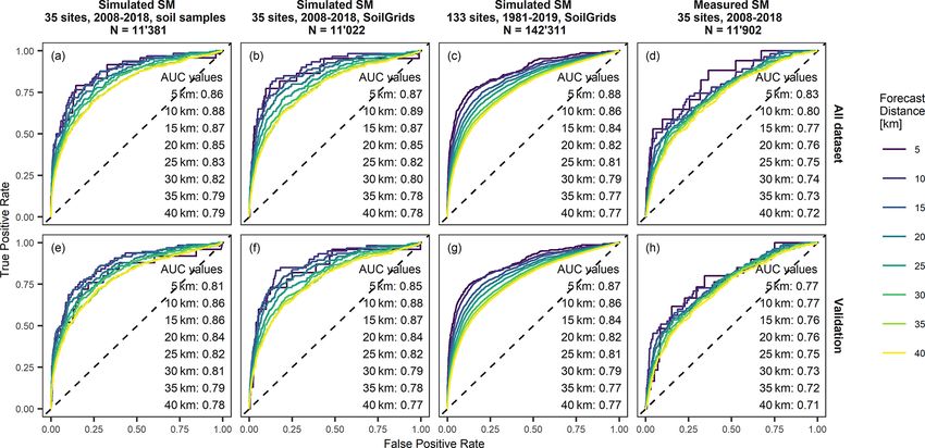
A. Wicki et al.: Simulated or measured soil moisture                                                                          4587

tions of using a 1D soil water transfer model for regional         ment of moist air masses on the Alps (CH2018, 2018; Hess
landslide early warning and highlights the strengths and           et al., 2014; Hilker et al., 2009).
weaknesses compared to using soil moisture measurements.
We use plot-scale soil hydrological simulations to be able         2.3   Soil moisture model
to directly compare the results to a landslide forecast model
based on in situ soil moisture measurements.                       In this study, the heat and mass transfer model CoupModel
                                                                   (Jansson, 2012) was used to simulate soil water transfer
                                                                   along a 1D virtual soil profile. The CoupModel has been used
2     Material and methods                                         extensively to simulate temporal soil moisture dynamics (e.g.
                                                                   Okkonen et al., 2017; Pellet et al., 2016; Scherler et al., 2010;
2.1    Study design                                                Wu et al., 2020; Wu and Jansson, 2013) and soil water bal-
                                                                   ance variations (e.g. Christiansen et al., 2006; Madani et al.,
The following section summarizes the design of this study.         2018; Walthert et al., 2015). In the context of landslide early
In a first step, soil moisture was simulated at 133 sites in       warning, parts of the CoupModel were used for soil moisture
Switzerland using a 1D soil moisture transfer model. Sec-          simulations within the Norwegian national forecasting ser-
ond, the forecast goodness for regional landslide activity was     vice for predicting rainfall-induced landslides (Krøgli et al.,
assessed by fitting and evaluating a statistical landslide fore-   2018).
cast model to observed shallow landslides. Finally, the land-         At the core of the model, two coupled differential equa-
slide forecast goodness was compared with a landslide fore-        tions for water and heat transport are solved, assuming that
cast model based on in situ soil moisture measurements avail-      flows are the result of gradients (Jansson and Karlberg,
able at a subset of the modelled sites. We applied a statistical   2011). The soil water flow, qw , follows Darcy’s law as gen-
framework previously developed to assess the information           eralized for unsaturated flow by Buckingham (1907).
content of in situ soil wetness information for regional land-
slide activity (Wicki et al., 2020), and we used the same soil
moisture monitoring data set compiled in the named study                           δψ
                                                                   qw = −Kw           −1 ,                                      (1)
for comparison with a measurement-based forecast model.                            δz
We focused on 1D soil moisture modelling because these                where Kw is the unsaturated hydraulic conductivity, ψ is
models permit high temporal resolution, detailed depth in-         the matric potential head, and z is the depth. Formulations to
tegration and a good representation of physical infiltration       simulate vapour flow and bypass flow in macropores are im-
processes, while still meeting the computational restraints.       plemented in the CoupModel as well but were not included
                                                                   in this study.
2.2    Study area
                                                                      From Eq. (1) and the law of mass conservation, the unsat-
The study area covers the entire country of Switzerland            urated water flow equation follows:
(Fig. 1) and, thus, an area of approximately 41 300 km2 . The      ∂θ    ∂qw
climate in Switzerland transitions from an oceanic (wet) cli-         =−     + sw ,                                             (2)
                                                                   ∂t     ∂z
mate in the west to a more continental (dry) climate in the
east of the country, and the presence of the Alps strongly         where θ is the soil water content, and sw is a source or sink
impacts the regional weather patterns. Hence, yearly precip-       term.
itation amounts are highly variable and range from less than          To solve the water flow equation, two soil characteris-
600 mm in some inner alpine valleys to more than 3000 mm           tic hydraulic properties need to be defined for each model
at high altitudes in the Alps. Precipitation falls throughout      layer, both of which are considered to be functions of the wa-
the year, with peaks during the summer months in most re-          ter content, i.e. the soil water retention curve, characterizing
gions, whereas the fraction of snow strongly depends on the        the relationship between matric potential and water content,
altitude (CH2018, 2018). Yearly evapotranspiration is high-        the unsaturated hydraulic conductivity function, describing
est in lowlands (up to 600 mm over grasslands) and continu-        the hydraulic conductivity as a function of water saturation
ously decreases to less than 250 mm at elevations higher than      (or matric potential), and the saturated soil hydraulic con-
2500 m a.s.l. (Menzel et al., 1999).                               ductivity. In this study, they were defined by the Mualem
   Landslides in Switzerland occur mostly along the northern       and Van Genuchten closed-form equations (Van Genuchten,
pre-Alps and south of the Alps (Ticino) due to the presence of     1980; Mualem, 1976) as follows:
susceptible geological formations (flysch, schist or Bündner                    θs − θr
schist and phyllite), thick soil and debris covers n the mod-      θ = θr +             m ,                                   (3)
erately steep hillslopes and the occurrence of intense rainfall              1 + (αψ)n
events (Schmid et al., 2004). Most landslides occur during
                                                                                                   −m 2
                                                                              1 − (αψ)n−1 1 + (αψ)n
the summer months due to short-term thunderstorm cells or          Kw = Ks                                 ,                    (4)
                                                                                                 m
long-standing precipitation events often caused by impinge-                             1 + (αψ)n 2

https://doi.org/10.5194/hess-25-4585-2021                                       Hydrol. Earth Syst. Sci., 25, 4585–4610, 2021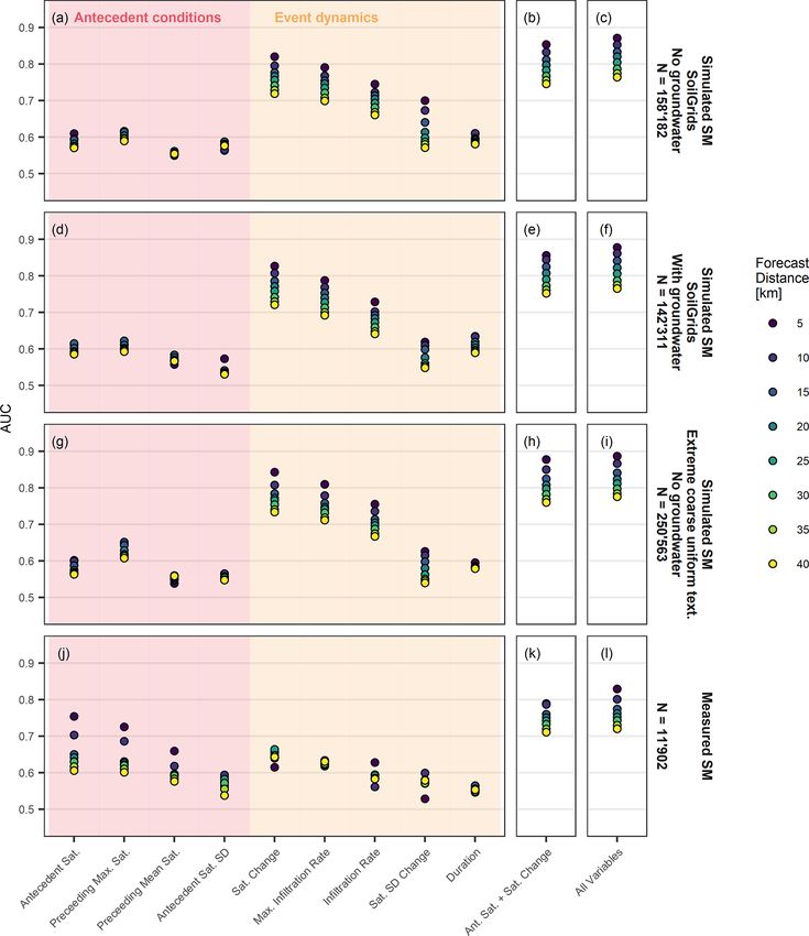
4588 A. Wicki et al.: Simulated or measured soil moisture
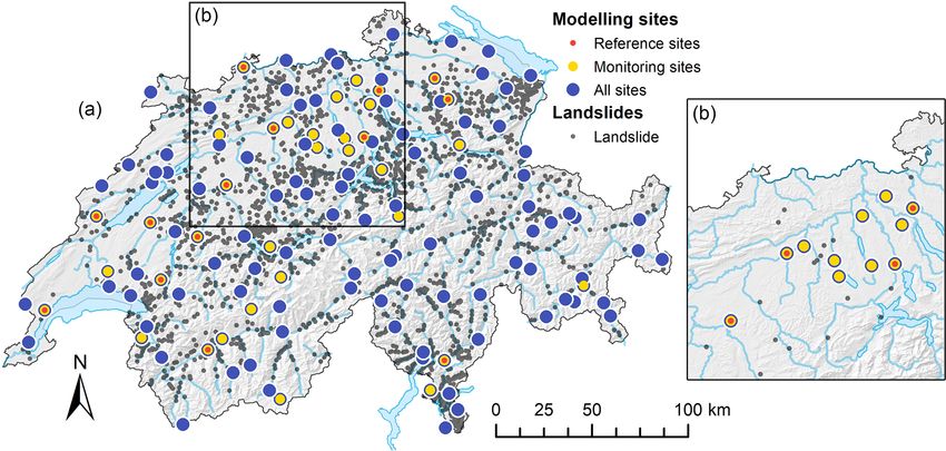
Figure 1. Map of Switzerland showing the locations of the soil moisture modelling sites (coloured points) and the landslide locations (black
points), including (a) all sites and all landslides of the entire study period from 1981 to 2019 and (b) a subset of sites and landslides that were
triggered during a series of rainfall events between 30 April and 3 May 2005.
where θr is the residual water content, θs is saturated water spiration components were calculated using the Penman–
content (equal to porosity), α, n and m = 1 − (1/n) are em- Monteith equation (Monteith, 1965), which is mainly gov-
pirical parameters, and Ks is the saturated hydraulic conduc- erned by aerodynamic and surface resistances (evaporation),
tivity. The heat flow equation follows Fourier’s law and ac- as well as stomatal resistance (transpiration). The potential
counts for conduction and convection of heat (Appendix A). transpiration is limited by the availability of soil water within
The differential equations are solved with a finite difference the rooting depth of the plants and is reduced by low ground
method (Euler integration), which requires a soil profile with temperatures. Finally, a snow cover may be built up based
a discrete number of layers having homogenous soil proper- on the air temperature at times of precipitation. Snowmelt
ties (Jansson and Karlberg, 2011). and refreezing were calculated with an empirical function de-
In the following, all other main processes represented in pending on air temperature, global radiation and surface heat
the CoupModel set-up are described. For a detailed descrip- flow (Jansson and Karlberg, 2011).
tion of the associated mathematical expressions, see Ap-
pendix A. At the lower boundary, water may leave the soil 2.4 Model set-up and parameterization
column by deep percolation. In the present study, two differ-
ent lower boundary conditions were applied; the first bound-
Soil moisture was simulated at 133 sites in Switzerland
ary condition assumes a nonsaturated soil profile. If a pre-
where meteorological data was available from an on-site or
defined pressure head is surpassed in the lowest layer, out-
nearby meteorological station, and each site was parame-
flow occurs as a function of the hydraulic conductivity (free
terized as a grassland location (all sites; Fig. 1a; Table 1).
drainage), whereas no flow occurs if the pressure head is be-
At a subset of 35 sites (monitoring sites), in situ soil mois-
low the specified limit. The second boundary condition may
ture measurements were available, which were used for
represent saturated conditions and a variable groundwater ta-
benchmarking the statistical landslide forecast model (see
ble. Here, outflow is calculated with a seepage equation de-
Sect. 2.6). At a subset of 14 selected sites (reference sites), in
pendent on the depth and spacing distance to a drain (Jansson
situ soil moisture measurements were used to assess the soil
and Karlberg, 2011).
moisture simulations from the CoupModel. They were se-
Infiltration capacity governs the infiltration of water at the
lected because they were located on the same plot as the me-
upper boundary, and it is a function of the top-most layer’s
teorological station and below grassland vegetation, i.e. the
saturated hydraulic conductivity and the pressure gradient to
soil moisture sites which were disregarded for model assess-
the surface. If the infiltration rate is exceeded by the wa-
ment were located at far distance from the meteorological
ter available for infiltration, or if over-saturation leads to
site (>2 km) and/or located in a forest and, thus, not repre-
an upward movement of the soil water, water may run off
sentative for the grassland parameterization.
laterally. Water loss by evapotranspiration consists of bare
The goal of this study was to define a common param-
soil evaporation and vegetation transpiration, which, in the
eterization set for all sites (i.e. no site-specific calibration
present study, was a mowed lawn. The individual evapotran-
was conducted) to be able to apply the model at sites where
Hydrol. Earth Syst. Sci., 25, 4585–4610, 2021 https://doi.org/10.5194/hess-25-4585-2021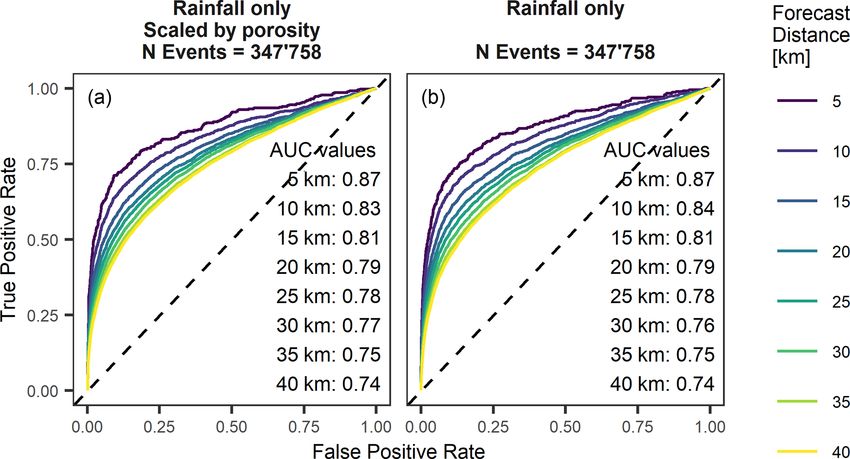
A. Wicki et al.: Simulated or measured soil moisture                                                                                4589

Table 1. Sets of sites, available data sets and number of sites.

               Sites set            Texture and bulk density information     Co-located soil moisture measurements    N sites
                                    SoilGrids    Soil samples
               All sites            Yes          No                          No                                          133
               Monitoring sites     Yes          Yes                         Yes                                          35
               Reference sites      Yes          Yes                         Yes (grassland only at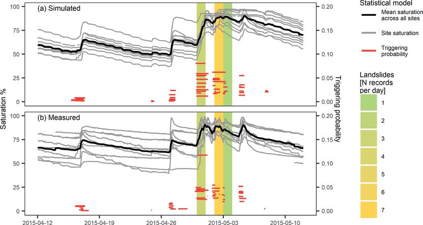
4590                                                                          A. Wicki et al.: Simulated or measured soil moisture

Figure 2. Soil texture splits (a, e) and soil hydraulic properties Ks (saturated hydraulic conductivity), n(Van Genuchten coefficient) and α
(Van Genuchten coefficient) (b–d, f–h) of the 35 monitoring sites averaged for the model layers in 0–40 cm (a–d) and 40–100 cm depth (e–h).
The point and box plot colours indicate different sources of information (soil samples, SoilGrids and uniform texture profiles).

land and Europe. At 14 sites, of which eight were in-                   riod). Both data gaps and spin-up periods, as well as the first
cluded in this study, co-located meteorological measure-                3 months after the spin-up period, were removed for the sta-
ments are taken in an open-field at less than 2 km dis-                 tistical analysis.
tance from the plots (Rebetez et al., 2018). (4) The
Swiss FluxNet initiative includes eight long-term ecosystem             2.6    Soil moisture data
sites with eddy covariance flux measurements in Switzer-
land (http://www.swissfluxnet.ch/, last access: 16 Febru-               For assessing the CoupModel performance and for compar-
ary 2021). In this study, meteorological measurements from              ison of the simulation-based forecast model with a forecast
two sites were included. (5) Finally, meteorological mea-               model based on measurements (see Sect. 2.8), soil moisture
surements from one site at the Rietholzbach research catch-             measurements from 35 sites in Switzerland were included in
ment were included, which is operated by the Land-Climate               the study (monitoring sites; Fig. 1a; Table 1). Soil moisture
Dynamics Group (ETH Zurich; https://iac.ethz.ch/group/                  is measured with TDR or capacitance-based sensors at vari-
land-climate-dynamics/research/rietholzbach.html, last ac-              ous depths along a soil profile, with the lowest sensors typ-
cess: 16 February 2021).                                                ically located at depths of 80–120 cm. The data set includes
   At each site, all available meteorological data were in-             sites from monitoring networks of various research institu-
cluded from the first point at which all five parameters were           tions and authorities, and measurements were available at the
available (as early as 1981) until the end of 2019. Data gaps           earliest from 2008 until end of 2018. The data set was com-
are generally short (hours to days) and were linearly in-               piled and described in detail in a previous study (Wicki et al.,
terpolated in the CoupModel, except for precipitation, for              2020).
which zero precipitation was assumed. Each complete time
series was replicated prior to the first measurement by 2 ran-
domly selected consecutive hydrological years (spin-up pe-

Hydrol. Earth Syst. Sci., 25, 4585–4610, 2021                                             https://doi.org/10.5194/hess-25-4585-2021
A. Wicki et al.: Simulated or measured soil moisture                                                                           4591

2.7   Landslide data                                               dation set approach, as opposed to the all data set approach,
                                                                   where the statistical model is fit to all the infiltration events.
Landslide records from the Swiss flood and landslide damage
database (Swiss Federal Research Institute WSL; Hilker et          2.9    Skill of the landslide forecast
al., 2009) were used to fit the landslide forecast model (see
Sect. 2.8). The database includes landslide events which were      To assess the forecast goodness of each specific statistical
identified from news articles in all of Switzerland since 1972.    model fit, receiver operating characteristic analysis (ROC)
Records include coordinates, the date and time of the event        was performed according to Fawcett (2006). First, a thresh-
(if known), and an event description.                              old was applied to reclassify the triggering probabilities of
   For this study, events recorded from 1981 until end of 2019     the infiltration events into the binary triggering classes land-
were included. Following the approach of Wicki et al. (2020),      slide triggering or landslide nontriggering. A confusion ma-
deep-seated and human-induced landslides (e.g. pipe breaks         trix was constructed between observed and modelled trig-
and road embankment slips) were removed if explicitly men-         gering classes counting the number of true positives (TPs),
tioned in the event description. Furthermore, if no time of oc-    true negatives (TNs), false positives (FPs) and false nega-
currence was specified, it was set to 12:00 Central European       tives (FNs). The true positive rate, TPR = TP / (TP + FN),
Time (CET), or, if the approximate timing was given in the         and false positive rate, FPR = FP / (FP + TN), were com-
event description, the timing was assumed (e.g. 09:00 CET          puted accordingly. To assess the overall potential of a model
for “in the morning”). In total, 2969 events were included in      fit for multiple thresholds, the threshold was varied 5000
this study (Fig. 1a), 1041 of which contained a precise time       times in equal steps between the minimum and maximum
information.                                                       triggering probability, thus resulting in 5000 confusion ma-
                                                                   trices. The 5000 TPR and FPR pairs were then plotted in a
2.8   Statistical landslide forecast model                         2D plot (ROC space), resulting in a cumulative curve (ROC
                                                                   curve) for which the area under the curve (AUC) was com-
To assess the information content of the simulated soil mois-      puted.
ture dynamics for regional landslide warning, a statistical           The forecast goodness of different model fits was assessed
framework was applied to the simulated soil moisture time          qualitatively by comparing the ROC curve and quantitatively
series. This framework was developed in a previous study,          by comparing the AUC value, which corresponds to the prob-
where it was applied to in situ measured soil moisture in          ability of listing a positive instance higher than a negative
Switzerland (for a detailed description, see Wicki et al.,         instance if sorted by the observed triggering class. A per-
2020). It included first a normalization of soil moisture val-     fect classifier plots near the top left corner of the ROC space
ues by the minimum and the 99.5 percentile values to repre-        (AUC = 1.0), whereas it is no better than random guessing
sent soil saturation, and the calculation of mean and standard     if it plots along the (0/0) to (1/1) diagonal (AUC = 0.5). To
deviation saturation at each soil profile for all model layers     assess the distance dependence of the forecast models, each
until 140 cm depth. At each profile, periods of continuous         model set-up was fit using eight different forecast distances
saturation increase (infiltration events) were then identified     ranging in equal steps from 5 to 40 km. We chose the ROC
automatically based on the mean saturation time series. Each       curve and AUC value as performance indicators because they
infiltration event was characterized by a set of event proper-     assess the general forecast goodness of a statistical model in
ties derived from both the mean and standard deviation time        contrast to many other performance indicators that quantify
series (see Table 2). Finally, infiltration events were flagged    the forecast goodness of specific threshold values (Piciullo et
as either landslide triggering or landslide nontriggering, pro-    al., 2020).
vided that a landslide was observed or not observed, respec-
tively, during the event period and within a specific distance     3     Results
from the modelling site (forecast distance).
   A multiple logistic regression model was then fitted to the     3.1    General model performance
set of infiltration events where the binary outcome variable
(i.e. the landslide triggering class of “yes” or “no”) was mod-    The performance of the soil moisture model and the corre-
elled as a function of the independent infiltration event prop-    sponding triggering probabilities according to the landslide
erties (explanatory variables). The logistic regression model      forecast model are illustrated for a model set-up using a
yields a probability for each infiltration event to belong to      lower boundary condition, with groundwater and soil hy-
the landslide triggering class (triggering probability). A five-   drological information from SoilGrids during a sample pe-
fold cross-validation (CV) scheme was applied to assess the        riod from mid-April to mid-May 2015 (Fig. 3a). During this
robustness of the model fit with equally sized folds and ran-      time period, a series of intense precipitation events led to
domly selected infiltration events. A total of four folds were     widespread landslide activity in central Switzerland, with nu-
used to fit the model, and the remaining fold was used as the      merous landslides observed from 30 April until 4 May 2015
to make predictions. This approach is referred to as the vali-     (black dots in Fig. 1b and colour-filled background in Fig. 3a,

https://doi.org/10.5194/hess-25-4585-2021                                          Hydrol. Earth Syst. Sci., 25, 4585–4610, 2021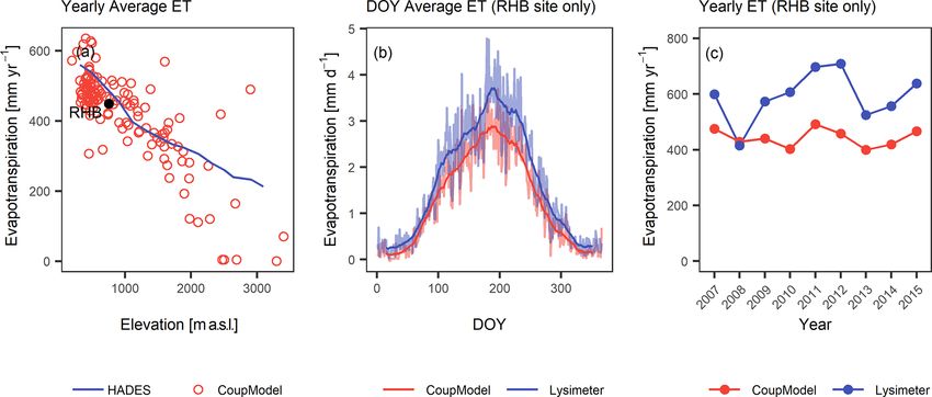
4592                                                                              A. Wicki et al.: Simulated or measured soil moisture

Table 2. List of event properties to describe infiltration events. To classify between triggering and nontriggering infiltration events, the nine
event properties marked with “x” are used. Time series of the mean of water saturation and standard deviation (SD) of saturation were used.

       Process domain            Event property description                         Name                      Profile mean     Profile SD
       Antecedent conditions     Saturation at the onset of infiltration event      Antecedent sat.                 x               x
                                 A 2-week preceding maximum saturation              2 week-prec. max sat.           x
                                 A 2-week preceding mean saturation                 2 week-prec. mean sat.          x
       Event dynamics            Saturation change during an infiltration event     Sat. change                     x               x
                                 Infiltration rate                                  Infiltration rate               x
                                 Maximum 3 h infiltration rate                      Max inf. rate                   x
                                 Event duration                                     Duration                        x

b). Profile saturation for a subset of 11 sites in the region of            3.2   Performance assessment of the soil hydrological
interest (coloured points in Fig. 1b) remained low and in-                        model
homogeneous prior to the landslide period. It increased to
near-saturated conditions and remained very wet for a couple
                                                                            The agreement between simulated and observed soil wet-
of days, which coincides with the period of landslide activ-
                                                                            ness was analysed for the 14 reference sites by the mean
ity. This development is confirmed by the landslide forecast
                                                                            error (ME) and coefficient of determination (R 2 ) statistics
model (fitted here for the 15 km forecast distance), which
                                                                            computed for the hourly soil moisture values. The skill of
shows a low triggering probability at the beginning of the
                                                                            the model set-up was generally solid but strongly varied
period (red horizontal lines; note that landslide probability is
                                                                            from site to site and with the depth of the sensors (Fig. 4a).
only computed for periods of saturation increase). Triggering
                                                                            Best agreement was found for the top-most sensors (median
probability increased significantly across all sites during the
                                                                            ME = 0.00 m3 m−3 ; median R 2 = 0.55–0.60). At depths of
period of landslide activity and descended again after that.
                                                                            30 and 50 cm, ME values were similar, but R 2 values were
While the relative triggering probability increases are con-
                                                                            lowest across all depths (median R 2 = 0.40–0.45). R 2 statis-
siderable, absolute probability values remain low even during
                                                                            tics were better at 80 cm depth (median R 2 = 0.50–0.55);
landslide-triggering events. This is the case for all infiltration
                                                                            however, mean error was greater than at all other depths (me-
events and can be attributed to an unbalanced data set (i.e. the
                                                                            dian ME = 0.02–0.05 m3 m−3 ), indicating too dry conditions
ratio of landslide triggering to landslide nontriggering events
                                                                            at the lower boundary, probably due to overestimation of
is very low; ratio not shown). It is commonly reported for lo-
                                                                            deep percolation. This skill is comparable to or slightly lower
gistic regression models with these types of data sets (King
                                                                            than reported skills for other soil moisture models used in
and Zeng, 2001).
                                                                            landslide early warning (e.g. Brocca et al., 2008; Thomas et
   These patterns can be compared to in situ soil moisture
                                                                            al., 2018) or for CoupModel set-ups with different purposes
measurements at the same sites and the corresponding land-
                                                                            (e.g. Conrad and Fohrer, 2009; He et al., 2016). However,
slide forecasts of a forecast model fitted to the soil moisture
                                                                            it has to be noted that these models are mostly validated for
measurements (Fig. 3b). Temporal evolution of the profile
                                                                            one or two sites only and were partially calibrated site specif-
saturation shows similar regional-scale patterns with variably
                                                                            ically.
saturated conditions during the first half of the sample pe-
                                                                               Not much difference in model skill was found between
riod followed by an increased saturation during the period
                                                                            using a lower boundary condition without groundwater
of landslide activity. Furthermore, the measurement-based
                                                                            (Fig. 4a) and with groundwater (Fig. 4b). When a lower
landslide forecast model shows a similar triggering proba-
                                                                            boundary with groundwater was defined, ME statistics re-
bility development to the simulation-based model, with sig-
                                                                            mained very similar (median ME = 0.00–0.05 m3 m−3 ), and
nificantly higher triggering probabilities for all sites during
                                                                            R 2 statistics slightly improved at the lowest depths (median
the days of observed landslide events compared to the peri-
                                                                            R 2 = 0.45 at 50 cm; median R 2 = 0.60 at 80 cm). Best model
ods prior to and after that. Yet, distinct differences are appar-
                                                                            fit of the groundwater-based model set-up was found for a
ent. The temporal evolution of simulated profile saturation
                                                                            parameterization indicative of a well-drained site.
appears to be more homogeneous between different sites; the
                                                                               Another important part in the parameterization is the site-
desaturation immediately after an infiltration event is slower,
                                                                            specific definition of the soil hydrological properties. Since
and it reaches drier conditions after sustained periods of no
                                                                            texture and bulk density information from soil samples were
infiltration. Triggering probabilities are generally lower for
                                                                            available for the monitoring sites only, they were derived
the measurement-based landslide forecast model.
                                                                            from a gridded product (SoilGrids) in order to be able to ap-
                                                                            ply the CoupModel with the same general set-up at all sites.
                                                                            Comparison of a soil-samples-based model set-up (Fig. 4a, b)

Hydrol. Earth Syst. Sci., 25, 4585–4610, 2021                                                  https://doi.org/10.5194/hess-25-4585-2021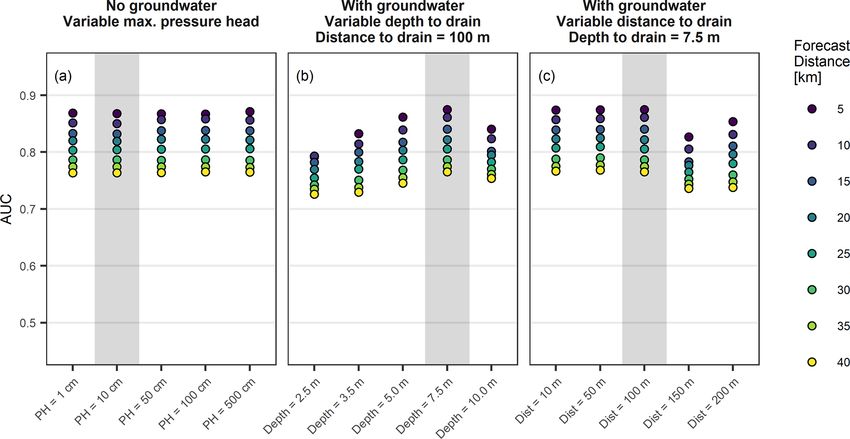
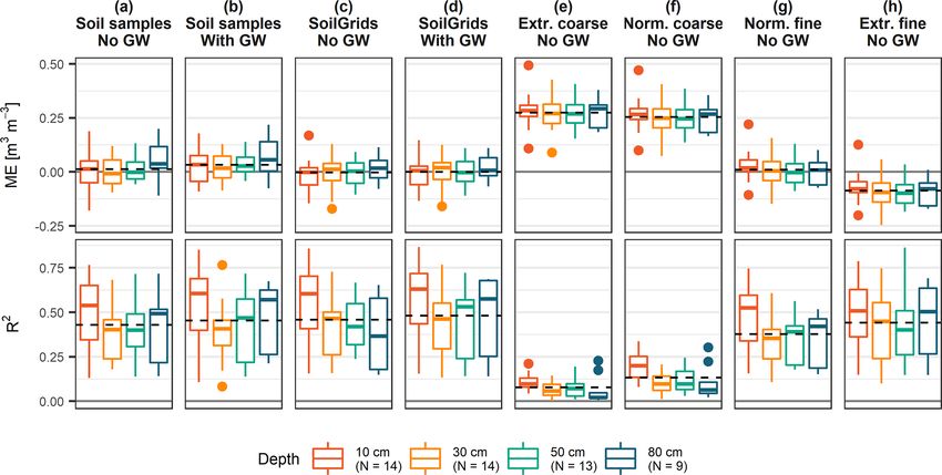
A. Wicki et al.: Simulated or measured soil moisture                                                                                       4593

Figure 3. Profile saturation (grey lines) of a selection of 11 sites in central Switzerland (as depicted in Fig. 1b), with the mean profile
saturation across all selected sites (black line), during a period of increased landslide activity in April and May 2015 for (a) simulated (lower
boundary with groundwater and soil hydrological properties from SoilGrids) and (b) measured soil moisture. The colour-filled background
denotes days with observed landslide events within 15 km of any of the sites, with the colour indicating the number of landslide records. The
red lines show the associated landslide triggering probability from the statistical model (based on the nine infiltration event properties listed
in Table 2) at each site, which was computed for periods of saturation increase only.

Figure 4. Goodness of fit of simulated versus measured soil moisture variation at the 14 reference sites, with the mean error (ME; top panels)
and coefficient of determination (R 2 ; bottom panels) indicated by sensor depths (different colours) for various CoupModel parameterizations
(a–h). Lower boundary conditions with and without groundwater (GW) are distinguished.

https://doi.org/10.5194/hess-25-4585-2021                                                 Hydrol. Earth Syst. Sci., 25, 4585–4610, 2021
4594 A. Wicki et al.: Simulated or measured soil moisture
with a model set-up based on SoilGrids information (Fig. 4c, Table 3. Percentage of country (area of Switzerland) and number
d) revealed very similar model skill, with a slightly decreased of landslides (percentage of all landslides recorded from 1981 to
mean error (median ME = 0.00 m3 m−3 at all depths) and 2019) covered by the soil moisture simulations and measurements
slightly larger range of R 2 values for the SoilGrids-derived as a function of the forecast distance used.
model set-up. This indicates that SoilGrids adequately rep-
All sites (133 sites) Monitoring sites (35 sites)
resents the regional variation in soil hydrological variability
and can be used to extend the model to all other sites. Fur- Forecast Percent of Percent of Percent of Percent of
thermore, the effect of having no regional variation in soil distance total area all landslides total area all landslides
hydrological properties was tested by deriving them from 5 km 22.6 26.8 6.4 7.1
the normal, fine-grained uniform texture profile (Fig. 4g). 10 km 65.6 73.7 22.1 26.0
Mean error statistics remained in a similar range (median 15 km 91.4 95.4 41.5 49.6
20 km 98.6 99.2 58.0 65.8
ME = 0 m3 m−3 at all depths); however, R 2 values were sig-
25 km 99.7 99.8 70.3 76.4
nificantly lower at all depths (median R 2 = 0.30–0.55). This 30 km 100.0 100.0 79.3 83.1
demonstrates the value of including regionally varying soil 35 km 100.0 100.0 87.0 88.6
hydrological properties. 40 km 100.0 100.0 92.6 93.7
Finally, large sensitivity of the model skill was found for
variation in the saturated hydraulic conductivity, which was
tested by deriving the soil hydrological properties from the term soil moisture measurements which have been partially
other, more extreme uniform texture profiles. Above-average running for up to 10 years (e.g. due to compaction of the soil
Ks values were defined for profiles representing extreme or enhanced root development around the sensors towards
coarse-grained and normal, coarse-grained soils (Fig. 4e, f), the end of the monitoring period). Furthermore, the differ-
and Ks values were below average for the extreme fine- ent sites each have different lengths of records which may
grained uniform texture profile (Fig. 4h). Model skill showed impact the homogeneity of the aggregated signal.
a very poor model fit for the coarse-grained profiles (me-
dian R 2 = 0.05–0.20) and very high mean error values in- 3.3 Performance of the statistical landslide forecast
dicative for too dry conditions (median ME = 0.25 m3 m−3 model
at all depths). Model fit was better for the extreme fine-
grained profile (median R 2 = 0.40–0.50), but ME statistics 3.3.1 Simulated versus observed soil moisture;
showed too wet conditions (median ME = −0.10 m3 m−3 at 35 monitoring sites
all depths). This indicates that the SoilGrids and soil samples
derived saturated hydraulic conductivity values are of an ad- ROC curves and AUC values for a CoupModel set-up with
equate order of magnitude. groundwater and, using soil hydrological properties derived
One important result of our soil moisture model assess- from soil samples, are shown in Fig. 6a. For comparison
ment was the fact that the deviation between model and mea- with a measurement-based statistical model fit, the data set
surement, i.e. the residuals, were not varying randomly, but contains the 35 monitoring sites only, and modelling peri-
had a seasonal trend (Fig. 5a, b; residuals were computed as ods were limited to the same periods for which soil mois-
mean daily values across all 14 sites). With a CoupModel ture measurements were available (2008–2018). ROC curves
set-up using SoilGrids information and a bottom boundary of all forecast distances clearly deviated from the (0/0) to
condition with groundwater, winter months showed posi- (1/1) line, and most AUC values were larger than 0.8, in-
tive anomalies (i.e. modelled soil moisture was drier than dicating that all forecast distances bore some information
observed), whereas negative anomalies (i.e. wetter than ob- content on the regional landslide activity. Forecast good-
served) were apparent during summer months. Both effects ness was strongly distance dependent, with short forecast
were more pronounced in near-surface layers. Furthermore, distances having a better forecast goodness (AUC = 0.86 at
near-surface layers showed wetter than observed anomalies, 5 km; AUC = 0.79 at 40 km; all data set approach). This is in
after the exceptionally dry summer in 2015, and negative good agreement to the results of Wicki et al. (2020) for mea-
trends not seen in the modelling. We explain the underes- sured soil moisture. The robustness of the statistical model
timation of the seasonal variation with an underestimation fit was assessed by comparison with the AUC values and
of evapotranspiration in summer (too wet conditions in sum- ROC curves of the validation set approach (Fig. 6e). Values
mer when evapotranspiration is high) and a generally faster were very similar for most forecast distances, indicating a
drainage than observed (too dry conditions in winter when robust model fit; however, robustness was slightly lower at
evapotranspiration is low). The overall negative trend in the short forecast distances, probably due to the low number of
anomalies (dashed lines in Fig. 5c) may be explained by landslide records (7 % of all landslides were within the 5 km
an underrepresentation of evapotranspiration in exception- radius of the 35 sites; see Table 3).
ally dry summers. However, it might as well be related to Compared to a statistical model derived from mea-
data quality issues and reduced homogeneity of the long- sured soil moisture (Fig. 6d, h), the number of infiltration
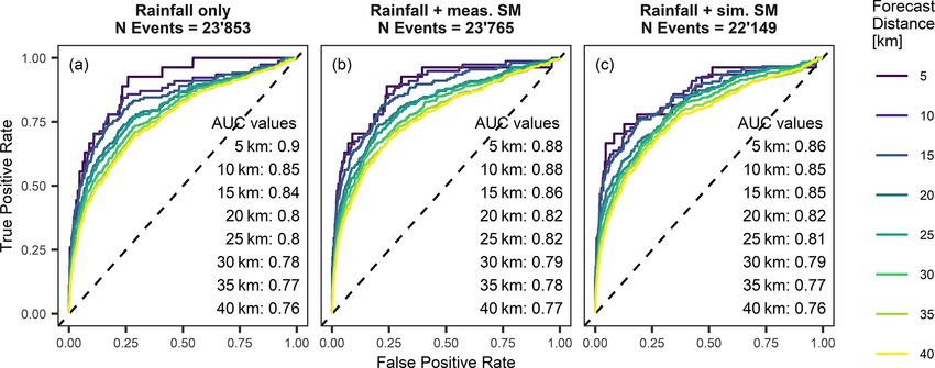
Hydrol. Earth Syst. Sci., 25, 4585–4610, 2021 https://doi.org/10.5194/hess-25-4585-2021A. Wicki et al.: Simulated or measured soil moisture 4595
Figure 5. Temporal evolution of, and seasonal variation in, mean daily residual volumetric water content (VWC) (a, b), i.e. the deviation
between simulated and observed soil water content, and mean daily measured (c, d) and simulated VWC (e, f). Means are calculated across
all 14 reference sites by sensor depths (different colours) for a CoupModel set-up using soil hydrological properties derived from SoilGrids
and a lower boundary condition with groundwater.
events was similar, yet the overall forecast goodness of the AUC = 0.78 at 40 km; all data set approach), and ROC curves
measurement-based forecast model was lower at all forecast followed a similar shape with more robust model fits at large
distances (AUC = 0.83 at 5 km; AUC = 0.72 at 40 km; all forecast distances. This finding is in line with the similar
data set approach). This is remarkable as the simulated soil goodness of fit as shown in the previous section and demon-
moisture was shown to contain specific uncertainty, partic- strates the validity of using soil hydrological properties de-
ularly related to the long-term water storage in the soil. We rived from SoilGrids. It permits the extension of the approach
explain the better forecast goodness of the simulation-based to all 133 sites, most of which had no in situ soil sample in-
landslide forecast model by a more homogeneous represen- formation available.
tation of infiltration characteristics in space (less influence
of local conditions, such as groundwater influence or prefer-
3.3.3 Increase in number of soil moisture sites
ential infiltration) and in time (no drift or trend as might be
observed for some erroneous or badly coupled soil moisture
sensors), as well as a more homogeneous site representation Extending the analysis to all 133 sites and to the entire in-
(number of sensors and depth levels included in the analysis). put data time period (1981–2019) resulted in a considerably
higher number of infiltration events (N = 142 311) and, thus,
3.3.2 Simulated soil moisture using in situ soil physical much smoother ROC curves (Fig. 6c, g). Furthermore, the
properties versus using SoilGrids model fits became very robust even at short forecast dis-
tances (i.e. same AUC values for the all data set and vali-
A similar forecast goodness resulted for a simulation with dation set approaches). AUC values were slightly lower than
SoilGrids-derived soil hydrological properties compared to when the 35 monitoring sites were used, but were in the same
a simulation with soil hydrological properties derived from range (AUC = 0.87 at 5 km; AUC = 0.76 at 40 km), and ROC
soil samples (Fig. 6b, f). AUC values and number of infil- curves bulged slightly less to the top, indicating a worse per-
tration events were in the same range (AUC = 0.87 at 5 km; formance for optimistic thresholds.
https://doi.org/10.5194/hess-25-4585-2021 Hydrol. Earth Syst. Sci., 25, 4585–4610, 20214596 A. Wicki et al.: Simulated or measured soil moisture
Figure 6. ROC plots and AUC values of landslide forecast model fits based on simulated soil moisture (SM) at the 35 monitoring sites,
including soil hydrological properties from soil samples (a, e) and SoilGrids (b, f) at all 133 sites and including soil hydrological properties
from SoilGrids (c, g), and based on measured soil moisture at the 35 monitoring sites (d, h). All CoupModel set-ups include a lower boundary
condition with groundwater. Panels (a)–(d) show landslide forecast model fits using all the data sets, whereas panels (e)–(h) show model fits
based on the fivefold cross-validation scheme.
Increasing the number of sites also increased the area and larger depth to drain (Fig. 7b) or a shorter distance to drain
number of landslides covered, as illustrated with Table 3. (Fig. 7c). This indicates a better landslide forecast goodness
When all 133 sites were used, almost the whole country for well-drained sites. As shown previously, the landslide
and all landslides were covered by using a 15 km forecast forecast goodness was similar for both a CoupModel param-
distance. When the 35 monitoring sites were used only (as eterization with or without groundwater, which is in line with
was the case for the measurement-based forecast model), the the very similar goodness of fit values for the two parameter-
same coverage is only possible when a 40 km forecast dis- izations.
tance is used. This is due to the lower number of sites and Low sensitivity of the landslide forecast model was found
because the available sites are distributed inhomogeneously, when using soil hydrological properties derived from uni-
including large gaps in alpine areas and in the eastern part of form texture profiles (Fig. 8), resulting even in a slight fore-
the country (Fig. 1a). cast goodness increase for the extreme and normal, coarse-
grained, uniform texture profiles. This is surprising since, by
3.3.4 Sensitivity of the landslide forecast model to the using uniform texture profiles, the regional variation in soil
definition of the lower boundary condition and hydrological properties is disregarded, and Ks values par-
soil properties tially deviate substantially from what can be expected in re-
ality, both of which were reflected with a substantially worse
The sensitivity of the landslide forecast model to changes in agreement with measured soil moisture in a previous sec-
the lower boundary condition was assessed by testing differ- tion. The reasons behind this are studied in more detailed
ent lower boundary parameterizations for CoupModel set-up in Sect. 4.
using all 133 sites (Fig. 7; grey boxes highlight the model pa-
rameterization that was chosen for the goodness of fit anal- 3.4 Most important explanatory variables for landslide
ysis). Low sensitivity of the landslide forecast goodness was forecast model
found for variations in the lower boundary conditions with-
out groundwater (Fig. 7a), which was defined by the max- In the previous section, the landslide prediction models were
imum pressure head of the lowest layer above which out- fitted, including all explanatory variables (also referred to
flow occurs as gravitational outflow. In contrast, when the as event properties) as listed in Table 2. In order to anal-
lower boundary was defined with a seepage function, the yse the contribution of individual explanatory variables to
landslide forecast goodness was very variable. Best results the overall forecast goodness, the landslide prediction model
were obtained for a fairly steep gradient to the drain, i.e. a was fitted to individual explanatory variables only, as illus-
Hydrol. Earth Syst. Sci., 25, 4585–4610, 2021 https://doi.org/10.5194/hess-25-4585-2021A. Wicki et al.: Simulated or measured soil moisture 4597
Figure 7. AUC values of landslide forecast model fits with different parameterizations of the lower boundary condition by varying (a) the
maximum pressure head of the lowest layer above which exfiltration occurs, (b) depth to the drain and (c) the distance to the drain. Grey
shaded model runs correspond to the CoupModel parameterization used in all other analyses.
a model fit including two explanatory variables only (an-
tecedent saturation and saturation change; second column)
and a model fit including all explanatory variables (third col-
umn) are plotted too. As expected, the forecast goodness of
individual explanatory variables was significantly lower than
when all explanatory variables were included. Furthermore,
model fits using the two explanatory variables antecedent the
saturation and saturation change had almost the same fore-
cast goodness as if all event properties were used.
When looking at individual explanatory variables in de-
tail, distinct differences become apparent between statisti-
cal model fits based on simulated and measured soil mois-
ture. For the simulation-based landslide forecast models, the
increase in the forecast goodness was mostly driven by ex-
planatory variables that describe the triggering event dynam-
ics (e.g. saturation change during the infiltration event, max-
imum 3 h infiltration rate, infiltration rate and standard de-
viation change; Fig. 9a, d, g). Inversely, for a measurement-
based landslide forecast model, explanatory variables related
to the antecedent wetness conditions were more important
Figure 8. AUC values of landslide forecast model fits based on (e.g. antecedent saturation and the 2 weeks preceding the
CoupModel set-ups with varying soil hydrological properties (de- maximum saturation; Fig. 9k).
rived from SoilGrids and uniform texture profiles) and a lower The worse performance of explanatory variables related to
boundary condition with groundwater. the antecedent wetness conditions for the simulation-based
forecast models can be related to the reduced ability of the
CoupModel set-up to reflect long-term seasonal water stor-
trated in Fig. 9 (first column), where AUC values are plotted age, as described previously (Fig. 5). The better forecast
for different statistical model fits. Explanatory variables can goodness of explanatory variables related to the triggering
be grouped into variables describing the antecedent wetness event dynamics of the simulation-based landslide forecast
conditions (shaded in red) and into variables describing the model can be explained by a more homogeneous site set-up,
infiltration event dynamics (shaded in orange). For reference,
https://doi.org/10.5194/hess-25-4585-2021 Hydrol. Earth Syst. Sci., 25, 4585–4610, 20214598 A. Wicki et al.: Simulated or measured soil moisture
no impact by very site-specific conditions (e.g. preferential macropores or concretizations (e.g. Or, 2020; Zhang and
flow, interaction with a local groundwater table and interac- Schaap, 2019). This may lead to an underestimation of Ks
tion with the vegetation) and by the elimination of measure- values which, in return, impacts surface runoff generation,
ment errors (e.g. sensor drift, sensor uncertainties and bad water infiltration and discharge (Fatichi et al., 2020).
sensor contact to surroundings). A second major source of uncertainty originates from the
The better performance of explanatory variables related to definition of homogeneous upper and lower boundary condi-
event dynamics compared to those related to antecedent con- tions. In general, seasonal soil moisture variation was under-
ditions was even more accentuated in the case of the extreme estimated, a problem also reported in other modelling studies
coarse-grained, uniform texture profile with a better forecast (Okkonen et al., 2017; Orland et al., 2020; Zhuo et al., 2019a)
goodness of most of the event-dynamics-related explanatory and which may be partially attributed to the definition of the
variables (Fig. 9g). Conversely, the antecedent saturation ex- vegetation and soil resistances and the potential evapotran-
planatory variable even showed a slight forecast goodness spiration calculation. Calibration is difficult due to missing
decrease. evapotranspiration measurements. We compared our evapo-
transpiration estimates with a countrywide evapotranspira-
tion estimation function for grassland locations depending
4 Discussion on elevation (Hydrological Atlas of Switzerland – HADES;
Menzel et al., 1999) and with estimations from lysimeter
4.1 Limitations of the soil moisture model measurements at the Rietholzbach site (RHB; Hirschi et
al., 2017). It was shown that evapotranspiration estimates
The soil moisture model incorporates errors and uncertain- slightly underestimated the HADES values; however, they
ties connected to the parameterization and the quality of the followed the same elevation dependence (Fig. 10a). When
input data, limiting the availability to reproduce soil mois- comparing with field lysimeter data, evapotranspiration es-
ture variation as observed with soil moisture sensors. A large timates were lower too (Fig. 10b) but followed the general
component of uncertainty originates from the definition of seasonal variation and showed similar interannual variation
the soil hydrological properties, which, in previous studies, except for the year of 2008 (Fig. 10c). This may explain the
were shown to have a great impact on simulated soil moisture underestimated drying out of the model compared with the
and landslide forecasts (e.g. Thomas et al., 2018). Here, un- observations as shown previously, which could be improved
certainty is added from both the definition of the site-specific by a more elaborate or site-specific vegetation parameteriza-
texture and bulk density values, as well as from the estima- tion. Nevertheless, the evapotranspiration data presented here
tion of the soil physical properties with a pedotransfer func- are only weakly representative and serve as a rough point
tion. No substantial differences in the goodness of fit of sim- of reference as they are based on simulations and show re-
ulated versus observed soil moisture were found between us- gional values (in case of HADES), and lysimeter measure-
ing soil hydrological properties derived from soil samples ments were available for one site only (RHB).
and those taken from SoilGrids. Yet, a decrease in the cor- At the lower boundary of the soil profile, the definition
relation coefficient was found when using the same normal, of well-drained conditions showed the best results. How-
fine-grained uniform texture profile for all sites. From that, ever, soil hydrological conditions might differ substantially
we can conclude that the soil hydrological property differ- for individual sites if shallow groundwater tables are present
ences between using soil samples and SoilGrids are smaller (Marino et al., 2020) or if soil depths vary between the sites
than the missing regionalization inferred by using a uniform (Anagnostopoulos et al., 2015); hence, a site-specific param-
texture profile only. This underlines the importance of using eterization might improve the goodness of fit with observed
regionally varying soil physical information for simulating soil moisture variation. While no seepage data on regional
soil moisture, which is often omitted due to a lack of field scales were available for calibration or validation, a site-
data or because too many parameters may lead to overfitting specific definition of lower boundary conditions could be
problems (e.g. Posner and Georgakakos, 2015; Zhao et al., achieved by consideration of nearby groundwater-level mea-
2019b). surements or regional groundwater distribution maps when
Larger uncertainty is probably introduced by the use of defining the depth and distance to drain for a lower boundary
a pedotransfer function to infer the soil hydrological prop- with groundwater.
erties from soil physical information. This point cannot be Finally, when comparing the goodness of fit with observed
validated directly since field data on site-specific soil hydro- soil moisture measurements, it has to be noted that the soil
logical properties is missing; however, the large ME spread moisture measurements bear uncertainties too and might be
across the 14 reference sites points towards partially incor- erroneous or contain a signal shift or trend due to bad contact
rect residual θr and saturated water content θs values. Fur- with the surrounding material, sensor deterioration or struc-
thermore, many studies highlight that pedotransfer functions tural changes in soil. Thus, a thorough quality assessment
incorporate a bias towards loamy agricultural soils and lack is needed when using soil moisture data for calibration or
a representation of soil structure, such as the presence of validation. Further to that, measurement uncertainties of the
Hydrol. Earth Syst. Sci., 25, 4585–4610, 2021 https://doi.org/10.5194/hess-25-4585-2021You can also read