Response of carbon and water fluxes to meteorological and phenological variability in two eastern North American forests of similar age but ...
←
→
Page content transcription
If your browser does not render page correctly, please read the page content below
Biogeosciences, 17, 3563–3587, 2020
https://doi.org/10.5194/bg-17-3563-2020
© Author(s) 2020. This work is distributed under
the Creative Commons Attribution 4.0 License.

Response of carbon and water fluxes to meteorological and
phenological variability in two eastern North American
forests of similar age but contrasting species composition
– a multiyear comparison
Eric R. Beamesderfer1,a , M. Altaf Arain1 , Myroslava Khomik1 , Jason J. Brodeur1 , and Brandon M. Burns1
1 School of Geography and Earth Sciences and McMaster Centre for Climate Change, McMaster University,
Hamilton, Ontario, L8S 4L8, Canada
a now at: School of Informatics, Computing & Cyber Systems, Northern Arizona University, Flagstaff,

Arizona, 86011, United States

Correspondence: M. Altaf Arain (arainm@mcmaster.ca)

Received: 22 November 2019 – Discussion started: 9 January 2020
Revised: 6 May 2020 – Accepted: 25 May 2020 – Published: 10 July 2020

Abstract. The annual carbon and water dynamics of two               riods that reduced ET at both stands, although the reduction
eastern North American temperate forests were compared              at the coniferous forest was relatively larger than that of the
over a 6-year period from 2012 to 2017. The geographic lo-          deciduous forest. If prolonged periods (weeks to months) of
cation, forest age, soil, and climate were similar between the      increased Ta and reduced precipitation are to be expected un-
two stands; however, stand composition varied in terms of           der future climates during summer months in the study re-
tree leaf-retention and shape strategy: one stand was a de-         gion, our findings suggest that the deciduous broadleaf forest
ciduous broadleaf forest, while the other was an evergreen          will likely remain an annual carbon sink, while the carbon
needleleaf forest. The 6-year mean annual net ecosystem pro-        sink–source status of the coniferous forest remains uncertain.
ductivity (NEP) of the coniferous forest was slightly higher
and more variable (218±109 g C m−2 yr−1 ) compared to that
of the deciduous forest NEP (200 ± 83 g C m−2 yr−1 ). Simi-         1   Introduction
larly, the 6-year mean annual evapotranspiration (ET) of the
coniferous forest was higher (442 ± 33 mm yr−1 ) than that          Temperate forests play a significant role in the global car-
of the deciduous forest (388 ± 34 mm yr−1 ), but with simi-         bon and water cycles through their photosynthetic CO2 up-
lar interannual variability. Summer meteorology greatly im-         take and through their evapotranspiration (ET) (Huntington,
pacted the carbon and water fluxes in both stands; however,         2006; Houghton, 2007). In eastern North America, temper-
the degree of response varied among the two stands. In gen-         ate forests are a significant sink of carbon and are an im-
eral, warm temperatures caused higher ecosystem respiration         portant element of future climate mitigation strategies; how-
(RE), resulting in reduced annual NEP values – an impact            ever, these forests have been going through transformations
that was more pronounced at the deciduous broadleaf forest          due to both natural and anthropogenic impacts for quite some
compared to the evergreen needleleaf forest. However, dur-          time (Bonan, 2008; Cubasch et al., 2013; Weed et al., 2013).
ing warm and dry years, the evergreen forest had largely re-        At the start of the 20th century, many of these forests were
duced annual NEP values compared to the deciduous forest.           cleared for agricultural purposes, effectively releasing car-
Variability in annual ET at both forests was related most to        bon into the atmosphere (Bonan, 2008; Richart and Hewitt,
the variability in annual air temperature (Ta ), with the largest   2008). With the rise of industrial development and move-
annual ET observed in the warmest years in the deciduous            ment of agricultural practices to other regions, many of
forest. Additionally, ET was sensitive to prolonged dry pe-         these agricultural lands were abandoned and subsequently

Published by Copernicus Publications on behalf of the European Geosciences Union.
3564                E. R. Beamesderfer et al.: Multiyear carbon and water flux responses to meteorology and phenology

reforested through natural regrowth and afforestation prac-        2     Methods
tices (Canadell and Raupach, 2008). Currently, much of the
forested area within the mixed-wood plains ecozone in the          2.1    Study sites
Great Lakes region of Canada and the USA is comprised of
reforested or plantation stands which are in different stages      The two forests are located within 20 km of each other, sit-
of growth (Wiken et al., 2011).                                    uated on the north side of Lake Erie in Norfolk County,
   Climate change and the associated changes in extreme            Ontario, Canada (Table 1). These forests are a part of the
weather events and the hydrologic cycle such as warmer             Turkey Point Observatory in association with the global
spring temperatures, intense heat and drought events in the        FluxNet program. The landscape in the region is domi-
summer, early snowmelt, reduced snowfall, or increased             nated by agricultural lands, while plantation and regenerated
freeze and thaw cycles in winter may impact the ability of         forests cover a small fraction (∼ 25 %) of the land cover;
these local forests to sequester carbon, and thus impact re-       accounting for the highest forest cover in southeastern On-
gional forest–atmosphere interactions (Bonan, 2008; Allen          tario. The broadleaf deciduous forest (from here on abbre-
et al., 2010; Teskey et al., 2015). However, climate change        viated and referred to as Turkey Point Deciduous, TPD)
will impact deciduous and coniferous forest ecosystems dif-        was naturally regenerated in the early 1900s from aban-
ferently due to their physiological differences. Even in de-       doned agricultural land on sandy terrain. The forest is un-
ciduous and coniferous forests of similar age, geographic lo-      evenly aged (70–110 years old) with a mean age of roughly
cation, climatic conditions, and soil properties, differences in   90 years. The stand is dominated by white oak (Quercus
the timing and rate of photosynthesis, ecosystem respiration,      Alba), with secondary hardwood species including red maple
and evapotranspiration may lead to asymmetries in the over-        (Acer Rubrum), sugar maple (Acer Saccharum), black oak
all forest productivity, water use, and hence longevity and        (Quercus Velutina), red oak (Quercus Rubra), white ash
survival. Consequently, regions once dominated by conifer-         (Fraxinus Americana), yellow birch (Betula alleghaniensis),
ous forests may yield to more deciduous species (Givnish,          and American beech (Fagus Grandifolia). Conifer species
2002; Bonan, 2008). Such a shift could disturb regional car-       only account for a minor component (∼ 5 %) of the total tree
bon and water budgets, as deciduous forests typically have         population (Kula, 2014). The understory is made up of young
shorter growing seasons and higher photosynthetic rates and        deciduous trees as well as Canada mayflower (Maianthemum
water use efficiencies when compared to coniferous forests         canadense), putty root (Aplectrum hyemale), yellow man-
(Givnish, 2002; Ciais et al., 2005). While many studies have       darin (Disporum lanuginosum), red trillium (Trillium erec-
examined the annual carbon and water fluxes within specific        tum), and horsetail (Equistum). The stand has been managed
land use and forest types, to date, only a handful of stud-        in the past with the last commercial harvesting occurring in
ies have compared these fluxes among similar-age deciduous         1984 and 1986, during which 440 and 39.97 m3 (wood vol-
and coniferous forests growing in close proximity, in similar      ume) of wood were removed, respectively. The specific har-
climatic and edaphic conditions (Gaumont-Guay et al., 2009;        vesting of white pine (Pinus Strobus L.; 106 m3 ), red pine
Baldocchi et al., 2010; Novick et al., 2015; Wagle et al.,         (Pinus Resinosa; 71.42 m3 ), poplar (Populus; 48.22 m3 ), and
2016). Even fewer studies have reported multi-annual time          dead oak (61.35 m3 ) also occurred from 1989 to 1994 (Long
series.                                                            Point Region Conservation Authority records). Since 1994,
   This study examined the carbon and water fluxes in two          no management activity has occurred in this stand.
eastern North American forest ecosystems of different tree            The evergreen needleleaf conifer forest, referred to as
species but similar age, climate, and edaphic conditions dur-      Turkey Point 39 (TP39 from here on), was planted in 1939 on
ing a 6-year period from 2012 to 2017. One stand was an            cleared oak-savanna lands. The dominant tree species in this
80-year-old (as of 2019) evergreen needleleaf forest, while        approximately 80-year-old stand are eastern white pine and
the other was a roughly 90-year-old broadleaf deciduous for-       balsam fir (Abies balsamifera L. Mill), making up 82 % and
est. The specific objectives of the study were to (1) exam-        11 % of the total tree population, respectively. The remaining
ine seasonal and interannual dynamics of carbon and water          7 % of trees are typical native eastern North American for-
exchanges in the two forests, (2) determine the impact of          est species, which includes white oak, black oak, red maple,
meteorological controls on overall forest productivities, and      wild black cherry (Prunus serotina Ehrh.), and white birch
(3) analyze and contrast the varying responses of the two dif-     (Betula papyrifera). The understory consists of young white
ferent forests to extreme meteorological events such as heat       pines, oak, balsam fir, and black cherry trees, as well as other
and drought.                                                       ground vegetation, including bracken fern (Pteridium aquil-
                                                                   inum), blackberry (Rubus spp.), poison ivy (Rhus radicans),
                                                                   moss (Polytrichum spp.), and Canada mayflower. The conifer
                                                                   forest has also been managed on two occasions. A thinning
                                                                   was performed in 1983 in which 4044 m3 of wood was re-
                                                                   moved from 38.6 ha land area (Ontario Ministry of Natural
                                                                   Resources and Forestry records). In the early winter of 2012,

Biogeosciences, 17, 3563–3587, 2020                                                     https://doi.org/10.5194/bg-17-3563-2020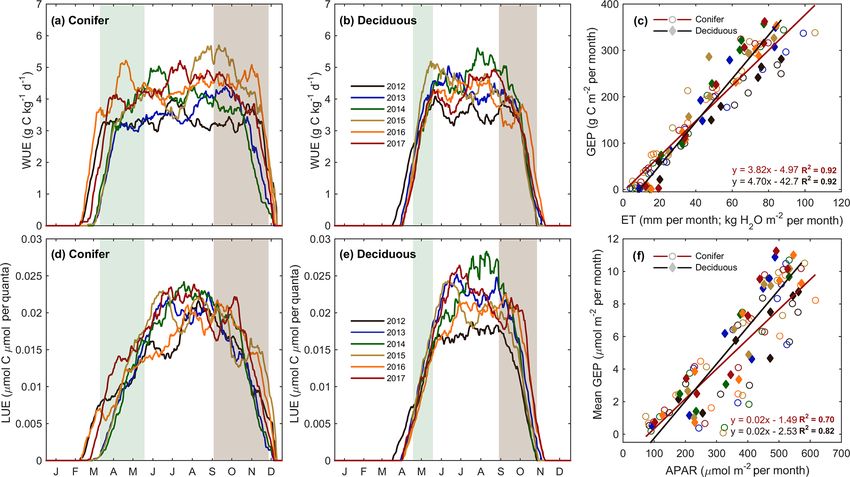
E. R. Beamesderfer et al.: Multiyear carbon and water flux responses to meteorology and phenology                                    3565

Table 1. Site characteristics of the deciduous (TPD) and coniferous (TP39) forest stands. The TP39 values in brackets indicate pre-thinning
(2003–2011) values, prior to the period of focus.

                                                   Turkey Point 1939 (TP39)          Turkey Point Deciduous (TPD)
                                                   42.71◦ N, 80.357◦ W               42.635◦ N, 80.558◦ W
                      Stand
                      Previous land use            Afforested on oak savanna,        Naturally regenerated on
                                                   cleared for afforestation         abandoned agricultural land
                      Age (in 2017)                78 years                          70–110 years
                      Elevation (m)                184                               265
                      DBH (cm)                     39.0 (37.2)                       23.1
                      Density (trees ha−1 )        321 (413)                         504
                      Tree height (m)              23.4 (22.9)                       25.7
                      LAI (m2 m−2 )                5.3 (8.5)                         8.0
                      Dominant species             Pinus strobus L.                  Quercus Alba
                      Secondary and understory     Abies Balsamea, Q. Velutina,      Acer Saccharum, A. Rubrum,
                                                   A. Rubrum, Prunus Serotina        Fagus Grandifolia, Q. Velutina,
                                                                                     Q. Rubra, Fraxinus Americana
                      Ground                       M. Canadense, Rubus Spp.,         Maianthemum Canadense,
                                                   Rhus Radicans, Ferns, Mosses      Aplectrum Hyemale, Equisetum
                      Soil
                      Drainage                     Well-drained                      Rapid to well-drained
                      Classification               Brunisolic grey brown luvisol     Brunisolic grey brown luvisol
                      Texture                      Very fine sandy-loam              Predominantly sandy
                      Bulk density (kg m−3 )       1.35 g m−3                        1.15 g m−3

the stand was again thinned by harvesting one-third of the              the Southern Norfolk Sand Plain, an area shaped by past ice
trees (2308 m3 ), leading to a reduction in stand density (Ta-          age glacial melt processes (Richart and Hewitt, 2008). Soils
ble 1). A subsequent study conducted by our group found that            at both sites are well-drained with a low-to-moderate water
while the 2012 thinning of the coniferous stand significantly           holding capacity (McLaren et al., 2008). Further soil and site
reduced the annual net ecosystem productivity (NEP) when                details can be found in Arain and Restrepo-Coupe (2005),
compared to the 9-year pre-thinning (2003–2011) mean an-                Peichl et al. (2010), and Beamesderfer et al. (2020). The cli-
nual NEP values, the post-thinning NEP was still within the             mate of the region is humid continental with warm, humid
range of interannual variability (Trant, 2014). Additionally,           summers and cool winters. The 30-year (from 1981 to 2010)
Skubel et al. (2017) reported that stand-level ET was not im-           mean annual air temperature and total precipitation mea-
pacted by the 2012 thinning, as increased soil evaporation              sured at the Environment Canada Delhi CDA weather station
and understory transpiration resulted due to a more open for-           (25 km north of the sites) is 8.0 ± 1.6 ◦ C and 997 mm, re-
est canopy. Ultimately, the objectives of this study did not            spectively. Total precipitation is normally evenly distributed
focus on examining the impacts of this disturbance.                     throughout the year, with 13 % of that falling as snow (Envi-
   While edaphic and climatic conditions are similar between            ronment and Climate Change Canada, 2019).
both sites, they differ in vegetation cover and canopy struc-
ture and physiology. The soils in each stand are predomi-               2.2   Eddy covariance and meteorological measurements
nantly sandy (greater than 90 % sand), classified by the Cana-
dian Soil Classification Scheme and FAO World Reference                 Half-hourly fluxes of water vapor and CO2 (Fc ) have been
Base as Brunisolic Grey-Brown Luvisol and Albic Luvi-                   measured continuously at TP39 and TPD using closed-path
sol/Haplic Luvisol, respectively (Present and Acton, 1984;              eddy covariance (EC) systems since 2003 and 2012, respec-
Lavkulich and Arocena, 2011). These sandy soils are part of             tively. This study examines the first 6 years (2012 to 2017)

https://doi.org/10.5194/bg-17-3563-2020                                                           Biogeosciences, 17, 3563–3587, 2020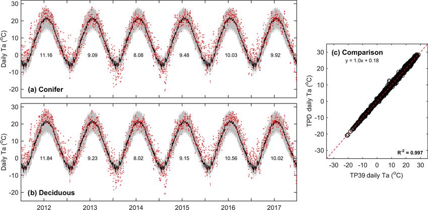
3566                E. R. Beamesderfer et al.: Multiyear carbon and water flux responses to meteorology and phenology

of data at the deciduous forest and the corresponding pe-          2.3   Meteorological and eddy covariance data
riod for the conifer forest. Measurements at both sites are              processing
still ongoing. The closed-path EC systems at each site con-
sist of a 3D sonic anemometer (CSAT3, Campbell Scientific          All meteorological and flux data were processed on lab-
Inc.) and an infrared gas analyzer (IRGA), an LI-7000 (LI-         developed software following the FluxNet Canada Research
COR Inc.) at TP39, and an LI-7200 (LI-COR Inc.) at TPD.            Network (FCRN) guidelines as described by Brodeur (2014).
The specific details of the EC systems are outlined in the         Meteorological variables were sampled at 5 s intervals and
Appendix (Table A1). At both sites, IRGAs are calibrated           averaged at a half-hourly scale. A two-step cleaning pro-
monthly using high-purity N2 gas for the zero offset and CO2       cess was used to remove outliers in half-hourly meteorolog-
gas (360 µmol mol−1 CO2 ; following WMO standards) for             ical data: coarse upper and lower thresholds were applied
the CO2 check.                                                     to half-hourly values to remove obvious outliers, and addi-
   The CO2 storage (SCO2 ) in the air column below the             tional erroneous half-hourly data were removed from time
EC system is calculated by vertically integrating the half-        series when instruments were known to be malfunctioning
hourly difference in CO2 concentrations. This calculation is       or visual inspection by multiple reviewers resulted in certain
completed for both the canopy and mid-canopy gas analyz-           agreement that an outlier was present. Missing meteorologi-
ers (Table A1). Half-hourly net ecosystem exchange (NEE,           cal data of all lengths were gap-filled using extant data for the
µmol m−2 s−1 ) is calculated as the sum of the vertical CO2        same half-hours from either (in order of preference) a second
flux (Fc ) and the rate of CO2 storage (SCO2 ) change in the       sensor at the site or an equivalent sensor from a nearby (1–
air column below the IRGA (NEE = Fc + SCO2 ). Horizon-             3 km away) station in the network (sites described in Peichl et
tal and vertical advection values are assumed to average to        al., 2010). This approach was supported by a very high corre-
zero over long periods and were not considered. Half-hourly        lation between variables (R 2 > 0.96). Linear regressions be-
net ecosystem productivity (NEP) is calculated as the oppo-        tween variables from different sources were used to correct
site of NEE (NEP = −NEE), where positive NEP (−NEE)                for any offset and gain discrepancies.
indicates net carbon uptake by the forest (sink), and negative        The same two-step cleaning process was also used to
NEP (+NEE) is carbon loss from the forest to the atmosphere        remove outliers from the flux data. For eddy-covariance-
(source).                                                          derived fluxes, the spike detection method described in Pa-
   Meteorological measurements have been conducted                 pale et al. (2006) was subsequently applied. After these qual-
alongside EC measurements during the entire measurement            ity control measures were applied, the mean flux data cover-
period at both sites. Air temperature (Ta ), relative humid-       age was 91 % (from 83 % to 94 %) at TPD and 88 % (from
ity (RH), wind speed and direction, downward and up-               79 % to 94 %) at TP39 over the 6 years of data collection.
ward photosynthetically active radiation (PAR), and the four-      Each time series was then subjected to a footprint filtering
components of radiation (Rn ) are measured at the specified        process, in which a footprint model (Kljun et al., 2004) was
EC sampling heights for both sites (Table A1). Soil tempera-       applied to exclude fluxes when greater than 10 % of the flux
ture (Ts ) and soil water content (θ ) are measured at 2, 5, 10,   footprint extended outside of the defined forest boundary
20, 50, and 100 cm depths in two soil pit locations at both        (Brodeur, 2014). This process removed approximately 32 %
sites. At TPD, precipitation (P ) is measured in a small forest    of half-hourly fluxes from TPD and 16 % from TP39. Finally,
opening, 350 m southwest of the tower. However, this anal-         nighttime (PAR < 100 µ mol m−2 s−1 ) fluxes were subjected
ysis used P data from an accumulation rain gauge (T-200B,          to friction velocity (u∗ ) filtering to remove half-hours where
GEONOR) installed 1 km south of TP39. All meteorological,          low turbulence may lead to underestimations by EC systems.
soil, and P data were recorded using data loggers with auto-       The moving-point test determination method (Reichstein et
mated data downloads occurring every half-hour on desktop          al., 2005; Papale et al., 2006; Barr et al., 2013) was used
computers located at the base of the scaffold walk-up towers       to estimate annual u∗ threshold (u∗ Th) values at each site,
located at each site.                                              and the nighttime half-hourly flux data were removed when
   Following an AmeriFlux visit to TP39 for an instrument          the measured friction velocity (u∗ ) was below the calculated
and data comparison (in 2019; data were processed after this       threshold (u∗ Th). The mean site-specific u∗ Th values were
study took place), the downward PAR sensor at that site was        0.40 m s−1 at TPD and 0.49 m s−1 at TP39. The resulting fi-
found to be identical to the AmeriFlux measurements. Con-          nal mean flux data recovery following both threshold filtering
sequently, downward PAR at TPD was thus underestimating            methods was 49 % (from 46 % to 53 %) at TPD and 53 %
(likely due to sensor differences, i.e., PAR-Lite vs. PQSI, and    (from 48 % to 57 %) at TP39 for the 6 years of measure-
their coefficients) actual PAR values. A correction factor of      ments. Confidence intervals (95 %) incorporating the effect
1.22 (slope between the two sites) was applied to daily mean       of random instrument error as well as systematic and ran-
PAR data at TPD for each year.                                     dom errors associated with the gap-filling process used for
                                                                   annual NEE estimates were calculated using a functional re-
                                                                   lationship with an annual gap percentage, developed for these
                                                                   sites by Brodeur (2014). The NEE model uncertainty ranged

Biogeosciences, 17, 3563–3587, 2020                                                   https://doi.org/10.5194/bg-17-3563-2020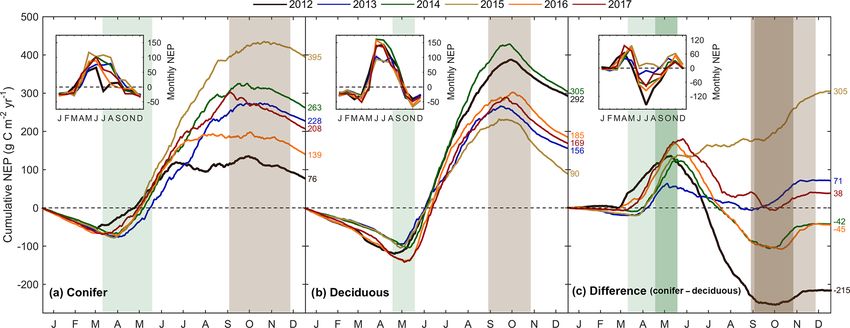
E. R. Beamesderfer et al.: Multiyear carbon and water flux responses to meteorology and phenology                          3567

from ±33–37 g C m2 yr−1 at TPD and ±31–36 g C m2 yr−1             (VPD), and θ0–30 cm , respectively. Parameters were optimized
at TP39. Furthermore, uncertainties in annual ET values to-       using the same approach described above. Finally, gaps in the
taling the sum of both measurement uncertainties and data         NEP time series were filled using the differences between the
gap-filling (as described by Arain et al. 2003) were esti-        filled GEP and modeled RE time series.
mated to be ±35–43 mm yr−1 at TPD and ±41–50 mm yr−1                  Following the aforementioned threshold and point clean-
at TP39.                                                          ing, gaps in the latent heat flux (LE), and therefore the mass
   NEE gap-filling and its partitioning into components of        equivalent evapotranspiration, were filled using an artificial
ecosystem respiration (RE) and gross ecosystem productiv-         neural network which utilized net radiation (Rn ), wind speed,
ity (GEP) were achieved using the methods described in Pe-        Ts5 cm , VPD, and θ0–30 cm (Brodeur, 2014). Following the ap-
ichl et al. (2010), which are summarized below. RE was            proach outlined by Amiro et al. (2006), any remaining gaps
assumed to be equivalent to NEE during nighttime periods          in LE data were filled using a moving-window linear regres-
(PAR < 100 µmol m−2 s−1 ) that passed both footprint and          sion method. Past studies examining the relationships be-
friction velocity filters. These values were used to model a      tween ET and meteorological variables for the forests of the
continuous RE time series based on a non-linear regression        Turkey Point Observatory have found Ta to largely drive ET,
with Ts5 cm and θ0–30 cm (depth-weighted average from mea-        with smaller secondary effects driven by VPD and θ0–30 cm
surements made at 5, 10, 20, and 50 cm depths) using the          during low-water or high-heat periods (McLaren et al., 2008;
functional form:                                                  MacKay et al., 2012; Skubel et al., 2015; Burns, 2017). All
                                                                  data processing and analyses were completed using MAT-
            (Ts5 cm −10)               1
RE = R10 × Q10 10        ×                            , (1)     LAB software (The MathWorks, Inc.).
                           1 + exp (a1 − a2 θ0–30 cm )

where parameters R10 and Q10 define controls of Ts5 cm on         2.4   Estimating effects of meteorological variables on
RE. The θ0–30 cm related controls are defined as follows:               carbon component fluxes

                                1
  (θ0–30 cm ) =                               ,          (2)    The partitioning models described above were further used to
                    1 + exp (a1 − a2 θ0–30 cm )
                                                                  explore interannual differences in controlling meteorological
where a1 and a2 are fitted parameters that describe a sig-        variables and their impacts on annual RE and GEP values at
moidal curve that ranges from 0 to 1 (Richardson et al.,          each site. In this analysis, the RE and GEP models (see Eqs. 1
2007). In this approach, the Ts5 cm component of the function     and 3 above, respectively) were parameterized for the phe-
defines a theoretical maximum half-hourly respiration rate        nologically derived summer months (end of greenup to the
based on soil temperature (i.e., driving variable), while the     start of browndown, defined in the next section) for all years
θ0–30 cm component modulates the resultant predicted value        (2012 to 2017). To overcome issues of equifinality that arose
as a function of the volumetric water content (i.e., scaling      when fitting the parameters of Eq. (1) and (3) to each year of
variable). Parameter values for Eq. (1) were derived for each     data, parameterization was performed as a two-step process,
site and year; values were estimated simultaneously using the     in which parameters describing “scaling” variable relation-
Nelder–Mead simplex optimization approach via the MAT-            ships (i.e., θ0–30 cm for RE; Ta , θ0–30 cm , VPD for GEP) were
LAB fminsearch function (The MathWorks, Inc). The esti-           fixed to all years of data, while relationships with “driving”
mated parameters were then used to model RE for all half-         variables (i.e., Ts5 cm for RE; PAR for GEP) were parameter-
hour periods using the measured values of Ts5 cm and θ0–30 cm .   ized to each year of data with other parameters fixed. Fur-
   Half-hourly GEP was derived as the difference between          thermore, the mean annual value for each scaling variable
modeled daytime RE and footprint-filtered NEE. Gaps in the        function was used to compare the quality of meteorological
GEP time series were filled using predicted values derived        conditions between years. Given that these variables scale
from the following relationship:                                  between 0 and 1, higher annual values (i.e., closer to 1) in-
                                                                  dicated that the variable was relatively more favorable for
          αPARAmax                                               RE or GEP production in that given year. To present this in
GEP =                ×          Ts5 cm ×     (VPD)
         αPAn + Amax                                              true relative terms, the annual values for a given functional
                                                                  relationship were normalized by the highest annual value.
     ×    (θ0–30 cm ) ,                                    (3)    Thus, reported annual values represent a proportion of the
                                                                  most favorable year. A similar metric was derived for the
where the first term is a rectangular hyperbolic functional re-   driving variables by modeling RE and GEP using the driv-
lationship between PAR and GEP, defined by the values of          ing relationships only (i.e., no scaling variables). Modeled
the photosynthetic flux per quanta (α, quantum yield) and         annual values were normalized by the highest one, thus cre-
the light-saturated rate of CO2 fixation (Amax ). The remain-     ating a relative annual score like that for scaling variables.
ing terms use the functional form introduced in Eq. (2) to de-    Finally, all metrics derived for scaling and driving variables
scribed the responses of GEP to Ts5 cm , vapor pressure deficit   in a given year were multiplied together to provide a measure

https://doi.org/10.5194/bg-17-3563-2020                                                  Biogeosciences, 17, 3563–3587, 2020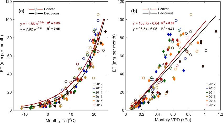
3568                E. R. Beamesderfer et al.: Multiyear carbon and water flux responses to meteorology and phenology

of the cumulative effect of all meteorological variables to a      the third derivatives estimated the start of the growing sea-
given component flux in a given year.                              son (SOS) and the end of the growing season (EOS). The
                                                                   start of the growing season (SOS) marked the end of winter
2.5    Definitions of key climatic and plant physiological         dormancy and the beginning of the spring season, leaf emer-
       variables                                                   gence/greenup. The phenologically defined spring season is
                                                                   defined as the period from SOS to EOG. The phenologically
In this study, we define the term drought similarly to Wolf        defined summer or peak carbon uptake period is defined as
et al. (2013), where drought periods are related to deficits in    the entire LOCC period from the final day of greenup (EOG)
precipitation, which impose either plant physiological stress      to the initiation of leaf senescence (SOB), bound by spring
due to decreased soil moisture (θ ) or impose stress due to        and autumn shoulder seasons. Finally, the resulting pheno-
stomatal closures in response to high VPD.                         logically defined autumn season is from SOB to EOS, with
   Two resource efficiencies were calculated at both forests       EOS marking leaf abscission and the end of photosynthetic
to compare the links between productivity and resource sup-        activity in autumn. The length of the overall growing season
ply in order to reveal differences in their responses to chang-    (LOS) was calculated as the number of days between SOS
ing climatic conditions. The amount of carbon fixed through        and EOS.
photosynthesis per unit of absorbed solar radiation, described        Lastly, the impact of climate on phenology was examined
as the photosynthetic light use efficiency (LUE) was calcu-        by the use of growing degree days (GDDs) and cooling de-
lated as follows:                                                  gree days (CDDs), in order to understand the thermal re-
         GEP                                                       sponse of each forest. GDD accumulation was defined as oc-
LUE =         ,                                             (4)    curring when the mean daily Ta was greater than 0 ◦ C, while
         APAR
                                                                   CDD were calculated using the daily mean Ta below a base
where GEP is equivalent to the carbon fixed through photo-         Ta of 20 ◦ C (Richardson et al., 2006). Cumulative GDD and
synthesis, and APAR is the portion of PAR that is absorbed         CDD were briefly considered in this analysis.
(Jenkins et al., 2007; Liu et al., 2019). The forest canopy ra-
diation budget used in the calculation of APAR is described
as follows:                                                        3     Results

APAR = PARdn − PARup − PARground,                           (5)    3.1    Meteorological variability

where PARdn is the incident PAR measured by PAR sensors            Air temperature measurements conducted above the canopies
mounted at the top of each tower facing skyward, and PARup         at both sites showed that the daily mean values of Ta at
is measured as reflected PAR by instruments mounted at the         TP39 (Fig. 1a) and TPD (Fig. 1b) behaved similarly (Fig. 1c)
same height as the PARdn sensor, but facing downward to-           over the study period. All years experienced annual mean
wards the forest canopy. PARground is the PAR transmitted          Ta greater than the 30-year mean (8.0 ◦ C). Record high Ta
through the canopy to a ground sensor located at 2 m height.       conditions (exceeding 30-year mean daily maximum values)
Furthermore, the forest-level water-use efficiency (WUE),          were measured throughout the majority of the year in 2012
describing the carbon fixed through photosynthesis per water       and during the summer of 2016. Cooler conditions domi-
lost, was calculated as the ratio of GEP to ET (Keenan et al.,     nated 2013 and 2014, while these years had a higher magni-
2013).                                                             tude of extreme cold days in winter (exceeding 30-year mean
    Using the methods of Gonsamo et al. (2013), we calcu-          daily minimum values), acting to decrease mean annual Ta .
lated phenologically derived seasons for each year for each        In 2015, 2016, and 2017, autumn warming was observed,
site. From half-hourly non-gap-filled data (calculated as the      with record Ta outside of the typical summer (June–August)
difference between modeled RE and measured non-gap-filled          period. Overall, daily mean Ta at both sites was almost iden-
NEE), the maximum daily photosynthetic uptake (GEPmax )            tical (Fig. 1c), highlighting the similar climate both forests
was calculated and fit using a double logistic function de-        were growing in during the study period.
scribed by Gonsamo et al. (2013). From the initial fit, a             Meteorological conditions at both sites were examined
Grubb’s test was conducted to statistically (p < 0.01) re-         over the study period. At TP39, APAR exhibited a simi-
move outliers in GEPmax data using the approach outlined           lar parabolic curve each year due to the seasonal ampli-
by Gu et al. (2009). With outliers removed, the function was       tude in PARdn and the continuous presence of an apparently
fit once more. This approach identified photosynthetic tran-       dense coniferous canopy promoting a nearly constant frac-
sition dates, hereafter described as phenological dates, using     tion (fPAR) of PARdn being absorbed (Fig. 2a). At TPD,
first, second, and third derivatives of the logistic curves. The   APAR exhibited lower values in the winter seasons when the
local minima of the second derivatives estimated the end of        forest remained leafless. The timing of the peak APAR at
greenup (EOG), the length of canopy closure (LOCC), and            TPD was similar to TP39, though it varied each year based on
the start of browndown (SOB), while the local maxima of            the annual timing of leaf-out and spring canopy development.

Biogeosciences, 17, 3563–3587, 2020                                                  https://doi.org/10.5194/bg-17-3563-2020
E. R. Beamesderfer et al.: Multiyear carbon and water flux responses to meteorology and phenology 3569
Figure 1. Daily above-canopy air temperature (Ta , red dots) measured from 2012 to 2017 at the (a) conifer forest (TP39) and (b) deciduous
forest (TPD), with the grey shading and black line corresponding to the 30-year Environment Canada (Delhi station) minimum and maximum
range of daily Ta and mean daily Ta , respectively. Values shown represent the annual mean Ta for each year of measurements. Also included
is the (c) comparison of daily Ta at TP39 and TPD.
Daily reductions in PARdn and APAR often resulted from TP39, while during all other times of the year θ at TP39 was
cloudy conditions and precipitation (P ) events (Fig. 2a). higher (Fig. 2g).
Fewer P events were measured during the first half of
2012 and most of 2015, 2016, and the late summer of 2017, 3.2 Phenological variability
as the latter three years had annual P less than the 30-year
mean (997 mm). Autumn P in 2012 helped the forests to re- The meteorological conditions had a significant impact on
cover from the record heat and water deficits, while 2013 the timing and duration of key phenological events, although
and 2014 experienced consistent rain throughout much of ultimately the response was governed by different leaf strate-
the year. Heightened daily VPD (Fig. 2b) was experienced gies of the various dominant tree species in each forest. The
throughout 2012 by both sites, with seasonal maximum val- phenological transition dates and seasons calculated from EC
ues measured during warm and dry conditions. In all years, flux data are shown in Table 2 and Fig. 3. The SOS varied
except for 2012 and the autumn of 2016, daily VPD at TP39 considerably between the two forests, with the SOS at the
was higher than at TPD (Fig. 2c). Annually, mean VPD was evergreen forest, TP39, beginning on average 38 ± 14 d ear-
on average about 0.04 kPa higher at TP39 than TPD, with lier than at the deciduous forest, TPD. TP39 experienced a
2012 being the obvious exception (Fig. 2c). larger variation in SOS dates, spanning a period of 26 d be-
Ts at 5 cm soil depth followed Ta closely (Fig. 1) with tween the earliest (10 March 2012; day of year, DOY, 70)
dampening effects evident at deeper (100 cm) soil layers and latest (6 April 2014; DOY 96) years, while TPD varied
(Fig. 2d). The differences in Ts5 cm were explained by the by 11 d between years.
species compositions of the two forests (Fig. 2e). At TPD, Growing degree days are a proxy used to assess the
when the deciduous forest was leafless in winter and spring, amount of heat the ecosystem has absorbed, as a result of
Ts5 cm was higher than at TP39 as the soil received more direct increasing air temperatures. The response of the forest to in-
radiation. However, during the summer and autumn of each creasing GDD was shown to be a trigger for the SOS. The
year, Ts5 cm at TP39 exceeded that of at TPD due to differ- total GDD from the start of the year (1 January, DOY 1) to
ences in canopy cover. Lastly, θ from 0–30 cm (θ0–30 cm ) fol- 6-year mean day of season growth (25 March; DOY 84) was
lowed similar patterns at both sites, with prolonged summer found to be highly correlated to SOS at TP39 (R 2 = 0.81),
θ declines in 2012, 2016, and 2017 (Fig. 2f). The magnitudes but not at TPD (Fig. 4a, b). GDD for DOY 117–127 (27 April
were again different, but each forest experienced similar de- to 7 May, which represents the range of the 6-year mean
clining θ and the subsequent recharging θ analogous to local SOS date ± 1 standard deviation) was found to significantly
P events. In the summer, θ was typically lower at TPD than influence the SOS at TPD (R 2 = 0.95), with a weaker in-
fluence at TP39 (DOY 73–95; R 2 = 0.76). This difference
https://doi.org/10.5194/bg-17-3563-2020 Biogeosciences, 17, 3563–3587, 20203570 E. R. Beamesderfer et al.: Multiyear carbon and water flux responses to meteorology and phenology Figure 2. Time series of daily mean meteorological variables measured at the conifer (TP39, red line) and deciduous (TPD, black dashed line) forests from 2012 to 2017, including (a, left) absorbed photosynthetically active radiation (APAR), (a, right) total precipitation (P ), (b) vapor pressure deficit (VPD), (c) the difference in VPD between the two forests (conifer – deciduous), (d) soil temperatures (Ts ) at 5 and 100 cm depths, (e) the difference in Ts between the two forests at both depths, (f) soil volumetric water content from 0–30 cm depths (θ0–30 cm ), and (g) the difference in θ between the two forests. likely reflects the different leaf strategies, in that evergreen With similar peak summer lengths, the forests began trees are ready to start photosynthesizing as soon as condi- senescence at similar times, though the length of autumn, the tions are favorable, while the deciduous trees still need to period from the SOB to the EOS, varied considerably be- grow their leaves once conditions are favorable, before com- tween the forests, due to differences in the timing of the EOS parable rates of photosynthesis are reached. Spring, defined (Fig. 3). Drought conditions in the summer of 2012 led both as the period from SOS to EOG, was more than double the sites to have the shortest autumns and earliest EOS (Figs. 2f length (69±14 d) at TP39 when compared to TPD (31±5 d). and 3). Conversely, late season warming in the autumns of However, even with largely different SOS and spring lengths, 2016 and 2017 helped to prolong the growing season at both the peak summer period, defined as the period between EOG sites, but the impacts of late season warming in 2015 were in spring and SOB in autumn, was essentially identical be- not as evident in shaping the timing of EOS (Figs. 1 and 3; tween the forests (Fig. 3). This period, spanning June, July, Table 2). and August, was found to be a key contributor to the net an- At both sites, the cumulative CDDs from DOY 230 to 290 nual productivity of each forest (discussed below). (mid-August to mid-October; loosely based on the range of Biogeosciences, 17, 3563–3587, 2020 https://doi.org/10.5194/bg-17-3563-2020
E. R. Beamesderfer et al.: Multiyear carbon and water flux responses to meteorology and phenology 3571
Table 2. The top section of the table contains the annual calculated phenological dates (reported as day of year) for both the conifer (TP39,
bold) and deciduous (TPD, italicized) forests from the year 2012 to the year 2017. Phenological dates were calculated following Gonsamo et
al. (2013) from eddy-covariance-measured GEPmax data. The 6-year mean values and standard deviations are included in the final column.
The resulting phenological periods (seasons) and their duration in days are also shown, in the lower section of the table.
Phenology transition dates 2012 2013 2014 2015 2016 2017 Mean
Start of season 70 96 96 91 74 79 84 ± 12
(SOS, bud-break) 120 116 127 118 126 125 122 ± 5
Middle of greenup 119 137 132 122 127 130 128 ± 7
(MOG, fastest greenup) 136 141 148 136 144 147 142 ± 5
End of Greenup 147 160 153 140 158 159 153 ± 8
(EOG, end of leaf-out) 145 155 160 146 154 159 153 ± 6
Peak of season 214 205 202 193 212 201 204 ± 8
(midpoint between EOG and SOB) 198 199 205 193 203 207 201 ± 5
Start of browndown 271 258 258 257 270 248 260 ± 9
(SOB, start of senescence) 257 249 255 249 262 261 255 ± 6
Mid of browndown 287 292 287 289 305 287 291 ± 7
(MOB, fastest senescence) 275 273 274 271 286 282 277 ± 6
End of Season (EOS) 314 351 338 345 366 354 345 ± 17
306 314 307 309 328 318 314 ± 8
Phenologically defined seasons 2012 2013 2014 2015 2016 2017 Mean
Spring 78 64 58 48 84 80 69 ± 14
(EOG – SOS) 25 39 34 28 28 34 31 ± 5
Summer (SOB – EOG) 124 97 105 117 112 89 107 ± 13
(LOCC, Length of Canopy Closure) 112 94 95 103 107 102 102 ± 7
Autumn (EOS – SOB) 43 94 80 89 96 106 85 ± 22
49 65 52 61 67 57 58 ± 7
Length of growing season (LOS) 245 255 242 254 292 275 260 ± 19
186 198 180 191 202 193 192 ± 8
dates in Oishi et al., 2018) were highly correlated to the EOS ble 3. Seasonal and total fluxes provide insight into each
at TP39 (R 2 = 0.84) and TPD (R 2 = 0.95) (Fig. 4e and f). stand’s ability to sequester carbon and release water over
Temperature responses in both the spring (i.e., GDD) and interannually comparable timescales. Annual photosynthe-
autumn (i.e., CDD) were much higher for TPD than TP39 sis (GEP) at the conifer forest (TP39) was the highest
(Fig. 4). These results suggest that warmer winter and early in 2017 (1709 g C m2 yr−1 ) and 2015 (1701 g C m2 yr−1 ),
spring (i.e., January to April) conditions will lead to an ad- while the lowest annual GEP was measured in 2012
vancement of the SOS in the conifer forest, but the same can- (1452 g C m2 yr−1 ) and 2013 (1501 g C m2 yr−1 ). GEP re-
not be said for the deciduous forest, whose SOS dates were ductions during these years were due to opposing influ-
heavily dependent on late-April–early-May growing condi- ences, with 2012 experiencing heat and drought conditions
tions. To a certain degree, both forests responded similarly in for most of the year and 2013 experiencing cooler Ta and
autumn; however, physiological constraints of the different the highest annual P (1266 mm), reducing PAR and there-
tree leaf strategies defined the overall differences in growing fore GEP (Fig. 3a). At the deciduous forest (TPD), similar
season lengths. GEP reductions were captured in 2012 (1198 g C m2 yr−1 )
but not in 2013 (1369 g C m2 yr−1 ), due to high photosyn-
3.3 Carbon and water fluxes thetic gains outside of the 2013 peak growing season (i.e.,
in the early spring and autumn periods). The highest an-
The water (evapotranspiration) and carbon (photosynthe- nual GEP at TPD was found in 2016 (1420 g C m2 yr−1 )
sis and respiration) fluxes were analyzed in both forests and 2017 (1447 g C m2 yr−1 ) due to warm summer condi-
from 2012 to 2017, with the seasonal patterns of these tions (Fig. 3b). Although 2014 had one of the shortest sum-
fluxes illustrated in Fig. 3 and cumulative fluxes in Ta-
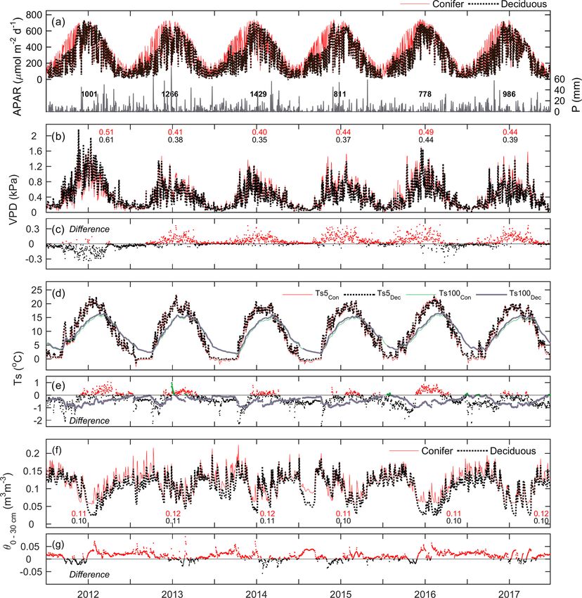
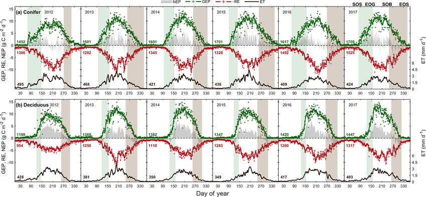
https://doi.org/10.5194/bg-17-3563-2020 Biogeosciences, 17, 3563–3587, 20203572 E. R. Beamesderfer et al.: Multiyear carbon and water flux responses to meteorology and phenology Figure 3. Time series from 2012 to 2017 of the daily total gross ecosystem productivity (GEP, green +), ecosystem respiration (RE, red +), net ecosystem productivity (NEP, grey shading), and evapotranspiration (ET, black, right) for the (a) conifer forest (TP39), and the (b) deciduous forest (TPD). Solid lines of GEP, RE, NEP, and ET are derived from 5 d moving averages of the measured data, while the colored values for each year correspond to annual GEP (green), RE (red), and ET (black) for each site. The annual EC-derived phenological spring (green shading) and autumn (brown shading) are included for each site, and can be found in Table 2. mers and the shortest overall growing season length of all lesser degree, the annual RE at TPD during 2017 was the years, high daily GEP rates were sustained through the sum- greatest of the 6 years (1317 g C m2 yr−1 ). Annually, the RE mer, resulting in the year having above-average annual GEP at both forests behaved similarly, with 2012 being the excep- (1382 g C m2 yr−1 ). In all 6 years, spring was the only season tion (Fig. 3b). The highest daily rates of RE at both sites were in which daily rates of GEP were similar between the forests, measured during the summer of 2013, coinciding with sim- as the advancement of SOS at TP39 did not statistically ben- ilar maximums in ET. In both cases, maximum rates of RE efit carbon uptake due to seasonal meteorological conditions and ET occurred following P events, as the soil was suffi- (i.e., low PAR, Ta , etc.) acting to limit photosynthesis. Us- ciently wet, helping to promote ET and enhance RE through ing the analysis of variance (ANOVA) technique, t tests were respiration pulses (suggested in Misson et al., 2006). Daily completed to evaluate statistical differences between the two summer RE was higher at TP39 in all years, with 2013 and groups (i.e., deciduous broadleaf vs. evergreen needleleaf) of 2015 being the exceptions. data. Summer and autumn daily GEP values were higher at The resulting balance between GEP and RE, net ecosys- TPD when compared to TP39 across the 6 years (p < 0.01). tem productivity (NEP), was found to be largely irregular be- In all years, TP39 annual GEP was greater than TPD due to tween sites during individual years due to site-specific differ- the longer growing seasons. ences in the timing, magnitude, and duration of daily fluctua- TP39 RE was highly variable in all years (Fig. 3a), tions in GEP and RE. The trajectory of growing season NEP with the greatest annual total RE values found in 2016 was strikingly different between sites (Fig. 3a and b). TPD (1492 g C m2 yr−1 ) and 2017 (1525 g C m2 yr−1 ). The annual (deciduous) captured consistently positive daily NEP (sink), RE during these years was about 100 to 200 g C m2 yr−1 while TP39 (conifer) was highly variable, with negative daily greater than during the other years. Cooler spring Ta and re- NEP (source) often occurring throughout the growing sea- ductions in RE during the summer of 2013 led to the low- son. The annual NEP in the conifer forest was the lowest est annual RE (1282 g C m2 yr−1 ) of the 6 years. While 2012 in 2012 (76 g C m2 yr−1 ) and 2016 (139 g C m2 yr−1 ), coin- encountered reduced ET and GEP during the summer, RE ciding with heat and drought stress in both years (Fig. 5a). was largely unaffected, leading to the third highest annual At TP39, July 2012 was the only month during the 6 years RE (1386 g C m2 yr−1 ). Conversely, the 2012 RE within the of measurements in which the peak summer growing sea- deciduous forest was greatly reduced, leading to an apparent son monthly NEP for either site was negative (Fig. 5a outlier (exceeding mean and standard deviation) in annual inset). The most productive years (largest annual sink) RE at that site (954 g C m2 yr−1 ). Similar to TP39, but to a at the conifer site were 2015 (395 g C m2 yr−1 ) and 2014 Biogeosciences, 17, 3563–3587, 2020 https://doi.org/10.5194/bg-17-3563-2020
E. R. Beamesderfer et al.: Multiyear carbon and water flux responses to meteorology and phenology                                     3573

Table 3. Seasonal and annual sums of eddy-covariance-measured carbon (GEP, RE, and NEP, g C m−2 yr−1 ) and water fluxes (ET, mm yr−1 )
from 2012 to 2017 for both the conifer (TP39, bolded) and deciduous (TPD, italicized) forests. The phenologically defined seasonal dates
were calculated using the timing of transitions in phenological dates, outlined in Table 2. The 6-year mean and standard deviations are also
included for each row.

                                   Season                  2012    2013    2014   2015    2016   2017         Mean
                       GEP sum     1 January to SOS            –      –       –       –      –       –            –
                                   Spring (SOS to EOG)       308    306     279    213     359     418     314 ± 70
                                                             104    197     165    117     129     174     148 ± 36
                                   Summer (EOG to SOB)       990    942    1070   1160    1014    930     1018 ± 86
                                                             942    949    1023   1006    1084   1070     1012 ± 59
                                   Autumn (SOB to EOS)       132    264     265    340     249     377     271 ± 85
                                                             147    239     200    240     219     213     210 ± 34
                                   EOS to 31 December          –      –       –       –      –       –            –
                                   Annual                  1452    1501    1601   1701    1617   1709    1597 ± 104
                                                           1198    1369    1382   1347    1420   1447     1360 ± 87
                       RE sum      1 January to SOS           66     83      78     79      82      81       78 ± 6
                                                             167    107     129    109     163     170     141 ± 30
                                   Spring (SOS to EOG)       205    205     169    122     233     276     202 ± 53
                                                              78    151     133    109     109     144     121 ± 27
                                   Summer (EOG to SOB)       908    718     809    790     888     735     808 ± 78
                                                             500    672     581    714     684     700     642 ± 84
                                   Autumn (SOB to EOS)       142    272     269    310     302     434     288 ± 94
                                                             138    269     196    259     266     252     230 ± 52
                                   EOS to 31 December         77     14      33     39       –      13      35 ± 26
                                                              82     64      84    110      55      65      77 ± 20
                                   Annual                  1386    1282    1345   1328    1492   1525     1393 ± 96
                                                            954    1250    1110   1283    1260   1317    1196 ± 138
                       NEP sum     1 January to SOS         –58     –74     –68    –73     –66    –66       –67 ± 6
                                                           –117     –79     –88    –82    –129   –130     –104 ± 24
                                   Spring (SOS to EOG)       103    101     110      92    128     144     113 ± 19
                                                              25     45      30       4     18      29      25 ± 14
                                   Summer (EOG to SOB)        80    223     262    374     127     196    210 ± 104
                                                             442    276     441    288     398     371     369 ± 73
                                   Autumn (SOB to EOS)       –12     –5      –6     33     –48     –51     –15 ± 31
                                                              16    –26       4    –18     –46     –37     –18 ± 24
                                   EOS to 31 December        –35    –12     –30    –24       –     –12     –23 ± 10
                                                             –68    –56     –79   –103     –51     –58     –69 ± 19
                                   Annual                     76    228     263    395     139     208    218 ± 109
                                                             292    156     305     90     185     169     200 ± 83
                       ET sum      1 January to SOS           22     23      11      19     13      15       17 ± 5
                                                              56     28      33      24     39      44      37 ± 12
                                   Spring (SOS to EOG)       105     97      67      65     85     106      87 ± 18
                                                              36     55      45      31     39      48       42 ± 9
                                   Summer (EOG to SOB)       315    277     260    286     249     210     266 ± 36
                                                             283    231     213    219     266     237     242 ± 27
                                   Autumn (SOB to EOS)        43     73      82      67     64      97      71 ± 18
                                                              45     63      50      66     69      64       60 ± 9
                                   EOS to 31 December         15      2       6       4      –       3         6±5
                                                              14      9      12      14     11      15        12 ± 2
                                   Annual                    495    468     421    436     408     424     442 ± 33
                                                             428    381     350    349     417     403     388 ± 34

https://doi.org/10.5194/bg-17-3563-2020                                                          Biogeosciences, 17, 3563–3587, 2020
3574 E. R. Beamesderfer et al.: Multiyear carbon and water flux responses to meteorology and phenology
Figure 4. Correlations between growing degree days (GDDs), cooling degree days (CDD), the phenological start of the growing season
(SOS), and the end of the growing season (EOS) from 2012 to 2017 at both the conifer and deciduous forests. Shown are (a) cumulative
GDDs from 1 January to the mean SOS at TP39 and (b) TPD, (c) cumulative GDDs from the mean SOS ± standard deviation at TP39 and
(d) TPD, and (e) cumulative CDDs from DOY 230 through 290 at TP39 and (f) TPD. Error bars represent the standard deviation of the data,
with R 2 , RMSE, and linear fit equations included for each correlation.
(263 g C m2 yr−1 ). While 2014 (305 g C m2 yr−1 ) was simul- tween sites benefited the extended photosynthesis measured
taneously the most productive year at the deciduous for- at TP39 (Fig. 5c).
est, 2015 (90 g C m2 yr−1 ) was the lowest annual sink, high- Within the evergreen conifer forest (TP39), annual ET
lighting the differences between sites (Fig. 5b). Similarly, was highest in 2012 (495 mm yr−1 ) and 2013 (468 mm yr−1 ).
the least productive year at TP39 (2012) was the second High Ta throughout much of the year and high summer VPD
most productive year at TPD (292 g C m2 yr−1 ). The cumu- caused 2012 to have the highest annual ET, while contin-
lative site differences in NEP were analyzed to focus on uous spring and summer P (Fig. 2a) allowed 2013 to sus-
seasonal differences (Fig. 5c). With earlier SOS at TP39, tain higher daily rates of ET (Fig. 3a). Cooler Ta during all
the conifer site quickly became a sink in spring, while the of 2014 (421 mm yr−1 ) and cooler Ta in the phenological
growing season had not yet begun at TPD. Following SOS, spring of 2016 (409 mm yr−1 ), combined with the lowest an-
daily NEP at TPD exceeded that at TP39 in all years ex- nual P (in 2016), caused these years to have the lowest ET
cept 2015 (p < 0.01). In the autumn, there was no statisti- for the conifer forest (Table 3). Within the deciduous forest
cal difference between sites, although as GEP ceased at TPD (TPD), 2012 (428 mm yr−1 ), 2016 (417 mm yr−1 ), and 2017
with leaf abscission, the cumulative difference in NEP be- (403 mm yr−1 ) had the greatest annual ET, coinciding with
the years with the highest annual Ta (Fig. 1b). In 2014, the
Biogeosciences, 17, 3563–3587, 2020 https://doi.org/10.5194/bg-17-3563-2020E. R. Beamesderfer et al.: Multiyear carbon and water flux responses to meteorology and phenology 3575
Figure 5. Cumulative daily sums of net ecosystem productivity (NEP) at (a) the conifer forest (TP39), (b) the deciduous forest (TPD), and
(c) the cumulative difference (conifer – deciduous), with appropriate monthly NEP sums in each panel inset, from 2012 to 2017. Green
shading in each panel corresponds to the site-specific 6-year mean phenological spring duration, while brown shading corresponds to the 6-
year mean phenological autumn duration (Table 2). Dark shading in panel (c) represents the deciduous forest seasons overlaid on the conifer
seasons. Cumulative annual values are shown for each site and year, with colors found in the key.
coolest year during the 6 years of measurements, annual ET early SOS (15 March; DOY 74) promoted prompt increases
(350 mm yr−1 ) was greatly reduced at TPD. While the ET of in spring GEP, when Ta and ET remained low. In autumn,
each forest ultimately responded differently to the local me- the years with extended growing seasons saw GEP increase
teorological forcings, on a few occasions, similar daily ET later in the year as ET decreased, leading to higher WUE.
rates were measured, coinciding with significant P events. At TPD, WUE was lowest in the warm years (i.e., 2012,
In the summer of 2013 (30 May to 19 July or DOY 150 to 2016, and 2017) due to increased annual ET, while the cool
200), high daily ET was measured at both sites, immediately and highly productive year of 2014 experienced the highest
following multiple daily P events exceeding 40 mm of rain summer and autumn WUE (Fig. 6b). In the 6 years of mea-
(Figs. 2a, 3a and b). Additionally, in 2015 (20 June to 10 July surements, highly significant (p < 0.01) linear relationships
or DOY 180 to 200), increased ET was measured at both of the monthly total ET and GEP (calculating WUE) were
sites following steady P events. Considering the 6 years as measured at both sites, with monthly WUE remaining rel-
a whole, phenological autumn was the only season in which atively constant (Fig. 6c; R 2 = 0.92). While monthly WUE
ET significantly differed between the sites. While the mean was similar between forests (Fig. 6c), WUE was higher at
autumn ET was greater at TP39, the shorter duration of au- TPD (4.70 g C kg−1 H2 O) when compared to that of TP39
tumn (Table 2) led to rates of daily ET to be higher at TPD as (3.82 g C kg−1 H2 O).
compared to TP39 (p < 0.01). In this case, the phenological The general LUE trends and deviations were statistically
autumn at TPD occurred when Ta remained high, while at comparable between the two forests. At both sites, 2014 and
TP39 autumn stretched later into the year when Ta and daily 2017 had the highest summer LUE, while reduced GEP at
ET were reduced. Both forests experienced similar variabil- both sites during the summers of 2012 and 2016 yielded
ity expressed as standard deviation in ET (33 and 34 mm), the lowest summer LUE (Fig. 6d and e). Across all years,
and in all years except for 2016, the ET of the conifer forest mean monthly linear relationships between GEP and APAR
exceeded that of the deciduous forest. yielded similar results, with larger variation (R 2 = 0.70) and
lower LUE at TP39 when compared to TPD (Fig. 6f; R 2 =
3.4 Forest light and water use efficiencies 0.82). Similarly, TPD had higher annual (data not shown) and
summer LUE (p < 0.01), although spring and autumn LUE
was similar at both sites.
The forest light and water use efficiencies (i.e., WUE and
LUE) were examined to understand the relationships be-
tween forest carbon uptake and site resources (i.e., water and 3.5 Meteorological controls on fluxes
light), illustrated in Fig. 6. At TP39, WUE was the highest
in the spring of 2016; the summers of 2014 and 2017; and Meteorological variables (i.e., Ta , PAR, θ , etc.) were ana-
the autumns of 2015, 2016, and 2017 (Fig. 6a). In 2016, an lyzed during the study period to better understand their im-
https://doi.org/10.5194/bg-17-3563-2020 Biogeosciences, 17, 3563–3587, 20203576 E. R. Beamesderfer et al.: Multiyear carbon and water flux responses to meteorology and phenology Figure 6. Annual smoothed (1-month moving average) time series of the (a) conifer (TP39) and (b) deciduous forest water use efficiency (WUE; GEP ET−1 ), and (c) monthly linear relationships between GEP and ET at both sites from 2012 to 2017. Similarly, light use efficiency (LUE; GEP APAR−1 ) calculations are shown for (d) conifer and (e) deciduous forests, with linear relationships (f) of monthly GEP and APAR also shown. Green and brown shading corresponds to site-specific 6-year mean phenological spring and autumn periods (Table 2), respectively. Linear fit equations and R 2 values also shown (c, f). pact on water and carbon fluxes within each forest. Consid- ing VPD was greater for the evergreen forest (R 2 = 0.82 vs. ering annual values, ET at the deciduous (TPD) forest was R 2 = 0.74; for TPD and TP39, respectively). found to be highly correlated (R 2 = 0.84) to annual mean Following similar annual timescales used in the ET com- Ta . A smaller secondary effect on ET (R 2 = 0.83; Table 4) parison, GEP, RE, and NEP were compared to meteoro- was found for winter and early spring (1 January to SOS) logical measurements for each site and season (Table 4). θ0–30 cm , which helped to explain the impact of winter soil In both forests, no significant relationships were found be- water storage and seasonal water availability on ET at the tween meteorological variables and annual GEP. In terms start of each year. At TPD, higher winter θ0–30 cm was mea- of RE at TP39, the years with the highest annual RE (i.e., sured in the years with the greatest annual ET. At the conifer 2016 and 2017) resulted from summer drought conditions, (TP39) forest, no strong relationships were found between as evident through prolonged reductions in mean summer annual ET values and seasonal or annual meteorological θ0–30 cm (R 2 = 0.89). The years with the lowest annual RE variables. However, monthly linear relationships of Ta and (i.e., 2013 and 2015) were ultimately the most productive VPD to ET were significant (p < 0.01) at both sites (Fig. 7). (largest annual carbon sink) and both measured the highest The evergreen conifer and deciduous broadleaf forests ex- mean summer θ0–30 cm . The annual NEP was correlated to the perienced similar increases in monthly ET with increasing length of spring (R 2 = 0.75), mean summer Ta (R 2 = 0.73), monthly mean Ta (Fig. 7a). While the evergreen forest saw and cumulative summer NEP (R 2 = 0.99). For the evergreen higher rates of ET compared to the deciduous forest, the conifer site, spring was shorter in years with the highest an- correlation of ET to Ta was greater for the deciduous forest nual NEP due to rapid photosynthetic development. Higher (R 2 = 0.95 vs. R 2 = 0.89; for TPD and TP39, respectively). mean summer Ta decreased annual NEP, highlighting the in- The response of monthly ET to monthly VPD was similar be- fluence of limitations due to heat stress. Lastly, summer NEP tween sites, as a mean monthly VPD of 1 kPa corresponded at TP39 was nearly identical to the annual NEP, stressing the to a monthly total ET of 104 and 97 mm at TP39 and TPD, re- importance of this period (roughly June, July, and August) in spectively (Fig. 7b). Overall, the correlation of ET to increas- shaping the annual carbon sink status of the forest. Biogeosciences, 17, 3563–3587, 2020 https://doi.org/10.5194/bg-17-3563-2020
You can also read