Multi-physics ensemble snow modelling in the western Himalaya
←
→
Page content transcription
If your browser does not render page correctly, please read the page content below
The Cryosphere, 14, 1225–1244, 2020
https://doi.org/10.5194/tc-14-1225-2020
© Author(s) 2020. This work is distributed under
the Creative Commons Attribution 4.0 License.

Multi-physics ensemble snow modelling in the western Himalaya
David M. W. Pritchard1 , Nathan Forsythe1 , Greg O’Donnell1 , Hayley J. Fowler1 , and Nick Rutter2
1 School   of Engineering, Newcastle University, Newcastle upon Tyne, NE1 7RU, UK
2 Department   of Geography and Environmental Sciences, Northumbria University, Newcastle upon Tyne, NE1 8ST, UK

Correspondence: David M. W. Pritchard (david.pritchard@newcastle.ac.uk)

Received: 10 August 2019 – Discussion started: 10 September 2019
Revised: 27 February 2020 – Accepted: 10 March 2020 – Published: 14 April 2020

Abstract. Combining multiple data sources with multi-              1   Introduction
physics simulation frameworks offers new potential to extend
snow model inter-comparison efforts to the Himalaya. As
such, this study evaluates the sensitivity of simulated regional   Snow plays a profound role in the climate system and sup-
snow cover and runoff dynamics to different snowpack pro-          ports water resources in many regions (Barnett et al., 2005;
cess representations. The evaluation is based on a spatially       Hall and Qu, 2006). As such, several applications depend on
distributed version of the Factorial Snowpack Model (FSM)          process-based models that approximate snow physics while
set up for the Astore catchment in the upper Indus basin. The      solving mass and energy balances. These include coupled
FSM multi-physics model was driven by climate fields from          land–atmosphere modelling, testing hypotheses about physi-
the High Asia Refined Analysis (HAR) dynamical down-               cal snow processes and catchment behaviour, and hydrologi-
scaling product. Ensemble performance was evaluated pri-           cal projections in non-stationary climates. Given the number
marily using MODIS remote sensing of snow-covered area,            of snow models in existence (e.g. Essery et al., 2013), under-
albedo and land surface temperature. In line with previous         standing the relative skill of different models and their suit-
snow model inter-comparisons, no single FSM configuration          ability for various uses is essential. This is reflected by the
performs best in all of the years simulated. However, the re-      succession of snow model inter-comparison initiatives over
sults demonstrate that performance variation in this case is       recent decades (Essery et al., 2009; Etchevers et al., 2004;
at least partly related to inaccuracies in the sequencing of       Krinner et al., 2018; Slater et al., 2001).
inter-annual variation in HAR climate inputs, not just FSM            While snow models have been evaluated in various con-
model limitations. Ensemble spread is dominated by interac-        texts, there has been little analysis of how different process-
tions between parameterisations of albedo, snowpack hydrol-        based models perform in the Himalayan region. Yet, vast
ogy and atmospheric stability effects on turbulent heat fluxes.    populations downstream of these water towers are vulnerable
The resulting ensemble structure is similar in different years,    to climate change impacts on snowmelt-derived river flows
which leads to systematic divergence in ablation and mass          (Immerzeel et al., 2010; Viviroli et al., 2011). Snow model
balance at high elevations. While ensemble spread and er-          analysis and inter-comparison would ultimately help to man-
rors are notably lower when viewed as anomalies, FSM con-          age these risks, but model input and evaluation are severely
figurations show important differences in their absolute sen-      impeded by data paucity. Indeed, deriving consistent, multi-
sitivity to climate variation. Comparison with observations        variate climate input fields in largely unobserved and highly
suggests that a subset of the ensemble should be retained for      variable mountain environments is a long-standing problem
climate change projections, namely those members including         (Klemeš, 1990; Raleigh et al., 2015, 2016). In part this ex-
prognostic albedo and liquid water retention, refreezing and       plains the proliferation of simple snow modelling in the re-
drainage processes.                                                gion, namely through (sometimes enhanced) temperature in-
                                                                   dex methods (e.g. Armstrong et al., 2019; Lutz et al., 2014;
                                                                   Ragettli et al., 2015; Stigter et al., 2017). There are a small
                                                                   but growing number of offline process-based, energy bal-
                                                                   ance model applications (i.e. not coupled to an atmospheric

Published by Copernicus Publications on behalf of the European Geosciences Union.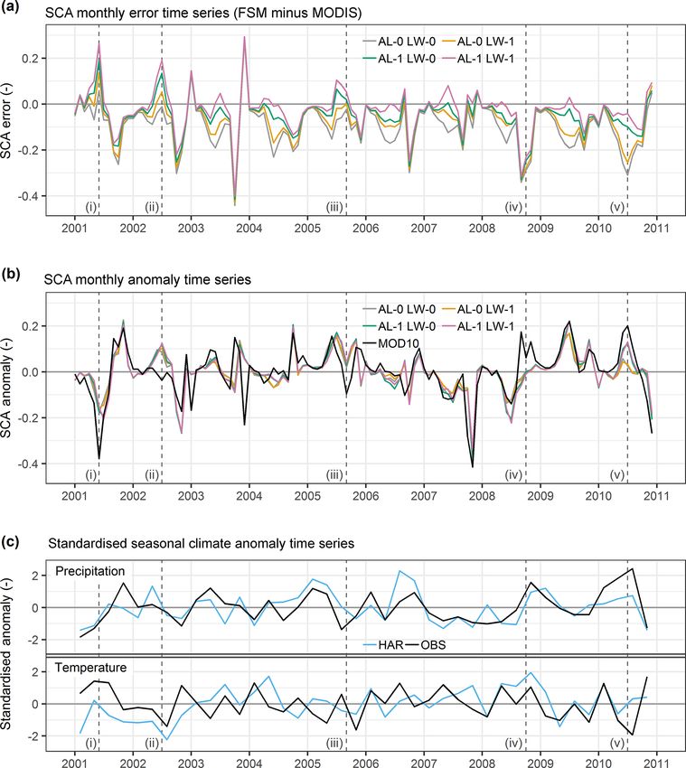
1226 D. M. W. Pritchard et al.: Multi-physics ensemble snow modelling in the western Himalaya
model), but these have focused only on single model struc- Therefore, this study uses recent progress in high-
tures, without detailed snow process evaluation (e.g. Brown resolution regional climate modelling, remote sensing and
et al., 2014; Prasch et al., 2013; Shakoor and Ejaz, 2019; ensemble-based snow modelling to assess snowpack model
Shrestha et al., 2015). formulations in a western Himalayan catchment. The study
In the face of these data challenges, developments in high- proceeds by using the High Asia Refined Analysis (HAR;
resolution regional climate modelling and remote sensing in- Maussion et al., 2014) dynamical downscaling product to
creasingly offer partial solutions. Several studies have now drive the Factorial Snowpack Model (FSM) multi-physics
successfully used dynamical downscaling to provide offline ensemble (Essery, 2015). The spatially distributed, high-
forcing for cryospheric and hydrological models in the Hi- resolution FSM simulations are then evaluated using a com-
malaya and other contexts (e.g. Biskop et al., 2016; Havens bination of multiple MODIS remote-sensing products and
et al., 2019; Huintjes et al., 2015; Tarasova et al., 2016). Sim- local observations. The aim of the study is to evaluate the
ilarly, the potential for remote sensing to support model eval- sensitivity of simulated snow cover and runoff dynamics to
uation by providing some constraints on both snow cover different snowpack process representations while also iden-
dynamics and the surface energy balance has been demon- tifying possible causes and implications of model perfor-
strated (Collier et al., 2013, 2015; Essery, 2013; Finger et al., mance variation. This contributes to the need for more large-
2011). Yet, studies combining these data sources for process- scale (basin-scale) model evaluations using unified frame-
based snow model applications are still few in number (see works (Clark et al., 2015; Essery et al., 2013) in a context
e.g. Quéno et al., 2016; Revuelto et al., 2018), especially in where accurately simulating snow processes is essential for
the Himalaya. Moreover, there has been little examination understanding cryospheric, hydrological and water resource
of how such approaches could support snow model inter- trajectories in a changing climate.
comparison for practical uses, such as water resource mod-
elling and management, as previous inter-comparisons have
focused primarily on site scales. More systematic studies are 2 Study area
needed to understand differences in snow model behaviour at
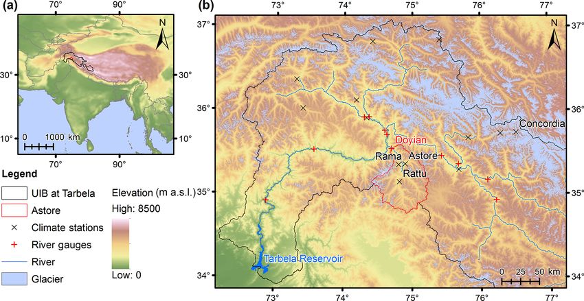
The study focuses on the steep, mountainous Astore catch-
the larger scales relevant to water resource applications and
ment, a 3988 km2 gauged sub-basin of the upper Indus basin
regional climate modelling (Essery et al., 2009; Krinner et
(Fig. 1). The mean elevation of the catchment is around
al., 2018).
4000 m a.s.l., with 57 % and 87 % of the area lying in the
Although regional climate modelling and remote sens-
elevation ranges 3500–4500 and 3000–5000 m a.s.l., respec-
ing offer increasing potential to support snow model inter-
tively. River flows are typically very low in winter, before
comparison in data-sparse regions, identifying appropri-
rising in spring and peaking in summer (June–July). Spring
ate model formulations remains challenging even in well-
and summer runoff is dominated by snowmelt, which is de-
instrumented contexts. In the SnowMIP and SnowMIP2
rived primarily from orographically enhanced snowfall in
inter-comparison studies, no single model emerged as opti-
the preceding winter and early spring (Archer, 2003). Show-
mal, with performance varying between locations and years
ing notable spatial correlation at the seasonal scale, much
(Essery et al., 2009; Etchevers et al., 2004; Rutter et al.,
of this snowfall originates from synoptic-scale low-pressure
2009). Similarly, recent inter-comparisons using more sys-
systems known as westerly disturbances (Archer and Fowler,
tematic ensemble frameworks have found that different
2004). Monsoon influences are small compared with the cen-
model configurations tend to show consistently good, poor
tral Himalaya. Together with the fact that glacier cover is
or variable performance, with no single best model identifi-
relatively limited, at around 6 % according to the Randolph
able (Essery et al., 2013; Lafaysse et al., 2017; Magnusson
Glacier Inventory 5.0 (Arendt et al., 2015), the strong corre-
et al., 2015). Model complexity, in terms of the number of
lation between winter precipitation and summer river flows
processes represented and the associated number of parame-
indicates that catchment runoff is primarily mass- rather than
ters, does not appear to be strongly (or necessarily positively)
energy-limited (Archer, 2003; Fowler and Archer, 2005).
related to skill or transferability in space and time (see also
However, energy constraints certainly affect intra-seasonal
Lute and Luce, 2017). Nevertheless, the systematic frame-
variability. The perennial snowpack that persists through the
works underpinning recent inter-comparisons are an impor-
summer is confined to small areas of very high elevation,
tant advance over earlier studies. By synthesising the array
while the glaciated extent is sufficient only to provide a mod-
of models in existence and eliminating implementation dif-
est contribution to late-summer river flows (Forsythe et al.,
ferences, these frameworks permit better quantification of the
2012). The ESA GlobCover 2009 product (Arino et al., 2012)
behaviour of different parameterisations and identification of
indicates that vegetation cover is relatively sparse, with the
where improvements may be possible (Clark et al., 2015;
catchment dominated by a mixture of bare ground, herba-
Krinner et al., 2018). The full potential of this approach has
ceous plants, and perennial snow and ice.
not yet been realised, especially in data-sparse mountain re-
gions.
The Cryosphere, 14, 1225–1244, 2020 www.the-cryosphere.net/14/1225/2020/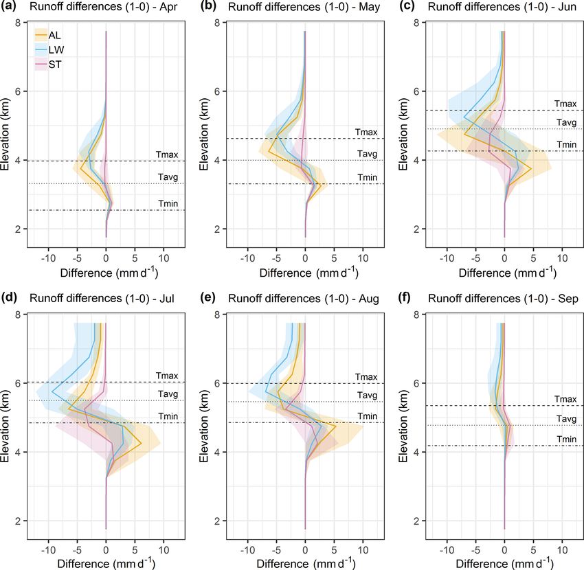
D. M. W. Pritchard et al.: Multi-physics ensemble snow modelling in the western Himalaya                                               1227

Figure 1. Location of study area and local measurement points. The regional context is indicated in (a). The Astore catchment and observation
locations (with labels for the most important sites in this study) are shown with topography and glacier extent in (b). The SRTM 90 m DEM
v4.1© (Jarvis et al., 2008) and Randolph Glacier Inventory 5.0© (Arendt et al., 2015) datasets are both licenced under a Creative Commons
Attribution 4.0 International License (CC BY 4.0).

3     Data and methods                                                   (Vionnet et al., 2012), HTESSEL (Dutra et al., 2010), ISBA
                                                                         (Douville et al., 1995), JULES (Best et al., 2011), MOSES
3.1     Model                                                            (Cox et al., 1999) and Noah-MP (Niu et al., 2011). For each
                                                                         process, the second option (1) may be considered generally
3.1.1    Factorial Snowpack Model (FSM) overview                         more physically realistic (i.e. more in line with conceptual
                                                                         understanding of the physical processes governing snowpack
FSM is an intermediate-complexity, systematic framework                  evolution) than the first option (0). For example, in the case of
for evaluating alternative representations of snowpack pro-              snowpack hydraulic processes, it is more realistic to include
cesses and their interactions (Essery, 2015). Constructed                liquid water retention, refreezing and drainage via a bucket
around a coupled mass and energy balance scheme, FSM was                 model (option 1) than to permit instantaneous drainage of
originally formulated as a one-dimensional column model                  liquid water instead (option 0).
with up to three layers, depending on the total snow depth.                 Analyses of FSM to date have shown that it gives en-
The model is based on the sequential solution of a set of                semble performance and spread comparable to larger multi-
linearised equations at each time step. The surface energy               model ensembles (Essery, 2015). As such, it has been used
balance is solved first. Turbulent heat fluxes are estimated             to support study design and inter-comparison in the ESM-
using the bulk aerodynamic approach. Heat conduction be-                 SnowMIP initiative (Krinner et al., 2018). Its value for test-
tween layers and to the substrate is calculated using an im-             ing new process representations in forest environments has
plicit scheme before layer ice and water masses are updated              also been demonstrated (Moeser et al., 2016), while Günther
to account for simulated rainfall, melt, sublimation, refreez-           et al. (2019) used FSM to delineate the influences of input
ing, drainage to successive layers and runoff from the base of           data errors, model structure and parameter values on simula-
the snowpack. FSM then updates layer densities and thick-                tion performance at an Alpine site.
nesses, accounting for snowfall and conservation of total ice
and liquid water masses as well as internal energy.                      3.1.2   Adaptations and implementation
   Within this framework, FSM offers alternative parameter-
isations of different snowpack processes. The five processes             While the core FSM subroutines used in this study remain
are as follows: (1) albedo evolution; (2) thermal conductivity           as described in Essery (2015), the model was adapted to per-
variation; (3) snow density change by compaction; (4) adjust-            form spatially distributed simulations on a regular grid, us-
ment of turbulent heat fluxes for atmospheric stability; and             ing climate inputs that vary in space and time. In this adap-
(5) liquid water retention, refreezing and drainage. With two            tation, each grid cell is treated as independent of all other
parameterisation options (0 or 1) for these five processes, the          cells. Inter-cell mass and energy transfers are not consid-
FSM ensemble includes 32 possible model configurations.                  ered, but the default parameterisation of sub-grid variabil-
Summarised in Table 1, the options synthesise approaches                 ity of snow cover as a function of snow depth is retained.
found in a range of widely applied models. These include                 In effect, each grid cell is considered to be a site for which
CLASS (Verseghy, 1991), CLM (Oleson et al., 2013), Crocus                the original FSM formulation is run. The adapted version of

www.the-cryosphere.net/14/1225/2020/                                                            The Cryosphere, 14, 1225–1244, 2020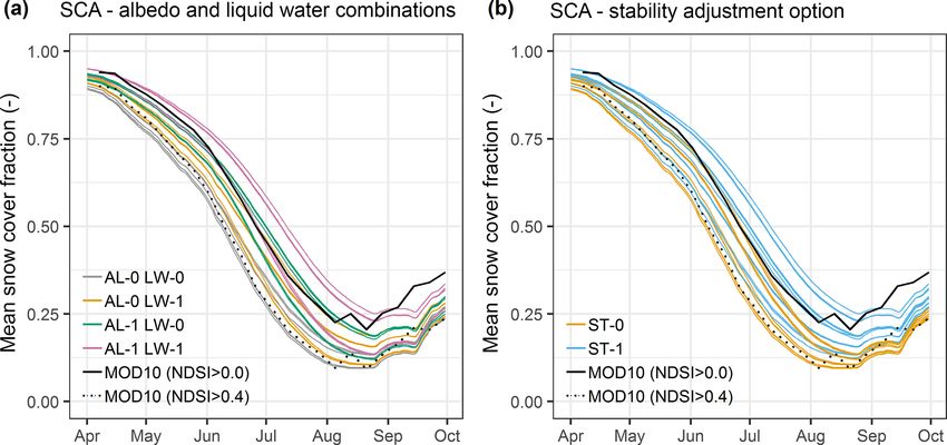
1228                            D. M. W. Pritchard et al.: Multi-physics ensemble snow modelling in the western Himalaya

Table 1. Summary of the process parameterisation options available in FSM. Full details are provided in Essery (2015). The short names and
abbreviations by which the processes are referred to in the text and figures are given.

  Process description            Short name                 Parameterisation 0        Parameterisation 1
  Snow albedo variation          Albedo (AL)                Diagnostic – function     Prognostic – decays with time and increases with
                                                            of surface temperature    snowfall
  Density of fresh snow and      Density (DE)               Constant                  Specified fresh snow density and compaction in-
  snowpack density evolution                                                          creases with time
  Liquid water storage,          Liquid water (LW)          Instant drainage,         Bucket model (drainage to layer below if liquid
  drainage and refreezing                                   no refreezing             holding capacity exceeded), with refreezing (and
                                                                                      latent heat release) accounted for
  Atmospheric stability          Stability (ST)             No adjustment for         Stability factor is a function of the bulk Richard-
  adjustment for turbulent                                  atmospheric stability     son number, which quantifies the extent to which
  heat fluxes                                                                         buoyancy suppresses shear production of turbu-
                                                                                      lent fluxes
  Thermal conductivity for       Thermal conductivity       Constant                  Function of density
  heat conduction                (TC)

the model is thus similar in principle to other widely applied,         the Weather Research and Forecasting (WRF) model (Ska-
distributed snow models when used without their snow trans-             marock et al., 2008). Although a seasonally varying cold bias
port options (Lehning et al., 2006; Liston and Elder, 2006a;            is present in the upper Indus basin, the HAR shows substan-
Marks et al., 1999). In line with the focus on snow cover dy-           tial performance in capturing many spatial and temporal pat-
namics and snowpack processes, the model does not simulate              terns in the near-surface climatology (Maussion et al., 2014;
other aspects of catchment hydrology, such as evapotranspi-             Pritchard et al., 2019). The HAR has also exhibited a good
ration from snow-free cells, the soil water balance or hydro-           representation of climate in several hydrological and glacio-
logical routing (subsurface, overland and channel flows).               logical modelling studies in neighbouring regions (Biskop et
   The simulations reported here use a 500 m horizontal res-            al., 2016; Huintjes et al., 2015; Tarasova et al., 2016).
olution grid and an hourly time step. Topography is derived
from the Shuttle Radar Topography Mission (SRTM) 90 m                   3.2.2    Bias correction and downscaling
digital elevation model (DEM) v4.1 (Jarvis et al., 2008). The
500 m spatial resolution is representative of hydrological and
                                                                        Near-surface air temperature fields were bias-corrected to
cryospheric modelling applications in the large basins of the
                                                                        reduce the HAR’s cold bias in the study area. The mean
Himalaya (e.g. Lutz et al., 2016) as well as extremely high
                                                                        bias was estimated using quality-controlled local observa-
resolution climate modelling (e.g. Bonekamp et al., 2018;
                                                                        tions from stations in the Astore catchment (Fig. 1b), which
Collier and Immerzeel, 2015). It is also consistent with sev-
                                                                        are maintained by the Pakistan Meteorological Department
eral of the MODIS products used for evaluation (Sect. 3.3).
                                                                        (PMD) and the Water and Power Development Authority
Spatial variation in land surface properties is ignored on the
                                                                        (WAPDA). Typical of data-sparse high-mountain regions, the
basis that glacier and vegetation (including forest) cover is
                                                                        available stations are situated in valley locations. The HAR
low (Sect. 2) and information on substrate properties is un-
                                                                        cold bias relative to these stations has been shown to be
available. The simulations use the default FSM model pa-
                                                                        closely related to issues in snow cover representation in the
rameters, which have been shown to reproduce much of the
                                                                        WRF simulations underpinning the HAR (Pritchard et al.,
spread in previous model inter-comparisons (Essery, 2015).
                                                                        2019), but some influence of local meteorological processes
3.2     Climate inputs                                                  such as cold air drainage cannot be ruled out, at least at some
                                                                        sites. More advanced bias correction approaches were tested,
3.2.1    High Asia Refined Analysis (HAR)                               including quantile-based methods, but these did not lead to
                                                                        improvements either in cross validation at station locations
Spatiotemporally varying input fields of rainfall, snowfall,            or model performance at the catchment scale. This is likely
air temperature, relative humidity, wind speed, surface air             due to the difficulty of fully characterising spatial and tem-
pressure, and incoming shortwave and longwave radiation                 poral variation in biases based on limited observations, es-
are based on the HAR (Maussion et al., 2014). The HAR                   pecially for less commonly measured variables. The mini-
is a 14-year dynamical downscaling of coarser global anal-              mal approach taken thus represents a realistic application of
ysis to 10 km over the Himalaya and Tibetan Plateau using               the data. It also has the advantage of retaining much of the

The Cryosphere, 14, 1225–1244, 2020                                                          www.the-cryosphere.net/14/1225/2020/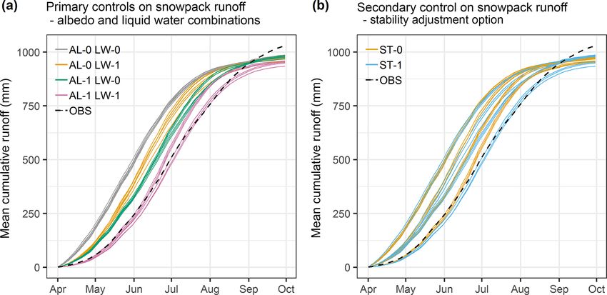
D. M. W. Pritchard et al.: Multi-physics ensemble snow modelling in the western Himalaya                                    1229

physical consistency of the HAR fields in terms of both inter-      western upper Indus basin (Fig. 1b) are used to estimate
variable and spatiotemporal dependence structures.                  fields for the other required variables (temperature, humid-
   For most of the climate variables, spatial disaggregation of     ity and incoming longwave radiation – see Sect. S1 in Sup-
the 10 km HAR fields to the 500 m FSM grid was conducted            plement). The purpose of these two alternative strategies is
using methods similar to those in the MicroMet meteorolog-          to indicate whether the main conclusions reached on snow-
ical pre-processor of SnowModel (Liston and Elder, 2006b)           pack process representations are unduly affected by the ap-
and those used by Duethmann et al. (2013). Specifically,            proaches described in Sect. 3.2.2.
for temperature, specific humidity, incoming longwave ra-
diation, pressure and (log-transformed) precipitation, linear       3.3   Model evaluation
regression was used each time step to relate each variable to
elevation, based on all HAR grid cells within the catchment         The model evaluation focuses primarily on snow cover dy-
(i.e. by regressing the simulated surface – or near-surface –       namics, with other variables considered to evaluate underly-
values against the elevations of the corresponding model grid       ing processes. Typical of the remote Himalaya, no local snow
cells). If the gradient term in the regression was significant      measurements for site-scale evaluation were available. The
at the 95 % confidence level, the values at each HAR cell           evaluation thus uses a number of MODIS remote-sensing
(10 km grid) were interpolated to a reference level using the       products (Collection 6) to assess the FSM ensemble over the
gradient. This spatial (horizontal) anomaly field was then in-      full simulation period (October 2000 to September 2014).
terpolated to the high-resolution FSM grid (500 m), and the         These include snow-covered area (SCA) derived from the
elevation signal was subsequently reintroduced using the re-        MOD10A1 daily snow cover product (Hall and Riggs, 2016).
gression gradient. This approach thus differs from MicroMet         Data with quality flags of 0 (best), 1 (good) and 2 (OK)
primarily by using gradients that can vary at each time step        were retained, and the widely used cloud infilling method de-
rather than applying a single climatological gradient for each      veloped by Gafurov and Bárdossy (2009) was then applied.
calendar month. For time steps when the gradient term in the        The analysis focuses primarily on SCA corresponding with a
regression was not statistically significant, simple interpola-     normalised difference snow index (NDSI) threshold of zero.
tion of the HAR field to the FSM grid was undertaken.               This indicates very limited or no snow cover in a pixel (Sa-
   Due to the pronounced topography of the study area, clear-       lomonson and Appel, 2004), which is consistent with the no-
sky shortwave radiation at the surface was estimated for the        snow threshold used to calculate modelled SCA.
500 m resolution DEM using a vectorial algebra approach                In addition, comparisons with MOD11A1 land surface
(Corripio, 2003). This approach accounts for the effects of         temperature (LST) are undertaken. To extend previous val-
slope, aspect, hill-shading and sky view factor. It has been        idations (e.g. Wan, 2014; Wan et al., 2004), an evaluation of
successfully applied before in this region (e.g. Ragettli et al.,   MOD11A1 at the Concordia site (Fig. 1b) in the neighbour-
2013) and was additionally checked against station measure-         ing Karakoram range is given in the Supplement (Sect. S2).
ments. The calculated clear-sky shortwave radiation fields          The evaluation shows that the product performs well com-
were adjusted to account for HAR-simulated cloud cover              pared with observed surface temperatures, with a relatively
effects. The cloud cover effects were estimated by using            low mean bias of −0.55 ◦ C. Spatial aggregates for LST were
spatially interpolated ratios of all-sky to clear-sky incoming      only calculated when 90 % of pixels had satisfactory quality
shortwave radiation at the surface, with both quantities from       retrievals, which are defined here as mandatory data quality
the HAR. This approach maintains consistency between vari-          flags of 00 (good). Additional evaluation of the FSM albedo
ables while capturing topographic influences, although direct       parameterisations presented in the Supplement also draws on
and diffuse partitioning and cloud variability are simplified.      the MCD43A3 and MOD10A1 surface albedo products, as
In addition, MicroMet itself was used to downscale wind             detailed in Sect. S3.
speed to the 500 m grid to take advantage of MicroMet’s                The study also uses quality-controlled daily river flows
routines for modulating wind fields according to topographic        over the period October 2000 to September 2010 recorded at
slope and curvature.                                                the Doyian gauging station by WAPDA (Fig. 1b). These data
                                                                    are used to provide some context on the volume, timing and
3.2.3   Uncertainty                                                 variability of catchment runoff. As the adapted FSM model
                                                                    does not simulate full catchment hydrology (Sect. 3.1.2), the
Given the low density of climate observations, biases and           use of the observed data is restricted to two cases: (1) an
other errors undoubtedly remain in the climate input fields.        indication of the timing of the rising limb of the annual
As such, two alternative input strategies were tested. The          hydrograph (and thus the timing of early snowpack runoff)
first strategy uses the same approach outlined in Sect. 3.2.2       for context and (2) an indication of the sensitivity of runoff
but simply forgoes bias correction of temperature. The sec-         to climate variability in the snow-dominated earliest part of
ond strategy retains the same approaches for precipitation,         the melt season (April), when flow pathways from the low-
incoming shortwave radiation and wind speed, but local ob-          elevation melting snowpack to the main channels are short,
servations from the Astore and other catchments in the north-       travel times are low and the influence of evapotranspiration

www.the-cryosphere.net/14/1225/2020/                                                     The Cryosphere, 14, 1225–1244, 2020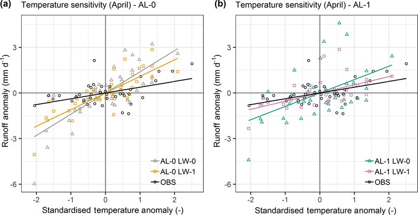
1230                             D. M. W. Pritchard et al.: Multi-physics ensemble snow modelling in the western Himalaya

Figure 2. Mean cumulative snowpack runoff for the high-flow season for each of the 32 ensemble members. In (a) each ensemble member
is coloured according to the combination of albedo (AL) and liquid water (LW) parameterisations it uses. In (b) each ensemble member is
coloured by its stability adjustment (ST) option. Observed total runoff (OBS; black dashed line) is shown for reference only (it is not directly
comparable with snowpack runoff – see Sect. 3.3).

is relatively small (Lundquist et al., 2005; Naden, 1992). The            tic albedo and apply the parameterisation of liquid water re-
modelled quantity considered is termed snowpack runoff,                   tention, refreezing and drainage processes (hereafter referred
which is defined as runoff from the base of the snowpack. It is           to as the liquid water parameterisation). The remaining two
thus different to surface melt, which may be subject to stor-             combinations of albedo and liquid water representations re-
age and refreezing processes before leaving the snowpack.                 sult in similar cumulative runoff curves, especially early in
Snowpack runoff is aggregated across all grid cells in the                the season (orange and green in Fig. 2a). This indicates that
catchment (or across subsets of the cells for selected analy-             a propensity for earlier, more rapid runoff when applying di-
ses) without any routing.                                                 agnostic albedo is offset by a delaying effect of the liquid wa-
                                                                          ter parameterisation. Conversely, a tendency to delay runoff
                                                                          in the prognostic albedo parameterisation is counteracted by
4     Results                                                             faster runoff due to instantaneous drainage. Interactions be-
                                                                          tween the albedo and liquid water parameterisations thus ap-
4.1     Mean ensemble structure                                           pear to govern whether a given option’s tendency to acceler-
                                                                          ate or slow snowpack runoff is compensated for or exacer-
4.1.1    Snowpack runoff                                                  bated.
                                                                             The next most important determinant of ensemble struc-
The evaluation begins by considering how the FSM ensemble                 ture for snowpack runoff is the stability adjustment option,
is structured on average at the catchment scale. For snowpack             whose significance increases later in the melt season, es-
runoff (as defined in Sect. 3.3), the ensemble shows notable              pecially in July. As noted above, Fig. 2a indicates that the
spread, which takes the form of groupings of ensemble mem-                spread in the ensemble groups increases with time. Cross-
bers (Fig. 2). Three groups of cumulative snowpack runoff                 referencing this with Fig. 2b illustrates that the stability ad-
curves are distinguishable early in the melt season (April and            justment is the main driver of the divergence. The separa-
early May) in Fig. 2, but the groups split and their spread               tion is particularly pronounced for the slowest-responding
increases to varying degrees thereafter, as melt rates acceler-           ensemble members (purple in Fig. 2a). In this case, not ap-
ate. Differences in snowpack runoff timing between groups                 plying a stability adjustment leads to more rapid snowpack
are substantial, with variation of around 1 month in the date             runoff from mid-June and earlier convergence with the other
at which the 25th, 50th and 75th percentiles of total seasonal            ensemble members, as evident from comparing the lower-
snowpack runoff are exceeded.                                             most orange and blue curves in Fig. 2b. In contrast, the
   Figure 2a indicates that the development of groups in the              adjustment effect is much less pronounced for the faster-
ensemble is primarily controlled by interactions between pa-              responding groups of ensemble members in Fig. 2a (grey
rameterisations of albedo and liquid water processes within               curves). Therefore, sensitivity to the stability adjustment not
the snowpack. The earliest, most rapid snowpack runoff oc-                only varies notably through the melt season but is also a func-
curs for members combining diagnostic albedo with instanta-               tion of the choices of albedo and liquid water parameterisa-
neous liquid water drainage (grey in Fig. 2a). In contrast, the           tions.
slowest-responding members (purple in Fig. 2a) use prognos-

The Cryosphere, 14, 1225–1244, 2020                                                              www.the-cryosphere.net/14/1225/2020/
D. M. W. Pritchard et al.: Multi-physics ensemble snow modelling in the western Himalaya 1231
Figure 3. Similar to Fig. 2 but for catchment snow-covered area (SCA). The two MODIS MOD10A1 series shown are based on normalised
difference snow index (NDSI) thresholds of 0.0 (solid line) and 0.4 (dotted line).
4.1.2 Snow-covered area (SCA) with MODIS (NDSI threshold of zero). Section S4 in the
Supplement explores how differential SCA errors could re-
Figure 3 indicates that the albedo, liquid water and sta- late to differences in the timing of early-season simulated
bility adjustment parameterisations are also the main influ- snowpack runoff and observed total runoff as well as what
ences on mean ensemble spread and structure in SCA. How- this could imply about the hydrological behaviour of the
ever, the dominance of albedo and liquid water processes is catchment.
lesser compared with snowpack runoff, especially later in
the melt season. By the annual SCA minimum in August, 4.2 Process evaluation
the stability adjustment comes to control ensemble structure
(Fig. 3b). Model configurations applying the adjustment ex- The analysis now explores the processes behind the struc-
hibit a markedly slower decline in SCA over the melt sea- ture of ensemble spread identified in Sect. 4.1 as well as how
son, which leads to an annual SCA minimum approximately far they can be assessed with independent data. This assess-
5 % higher. Spatially, this difference is largely found at high ment is based in part on Table 2, which summarises the mean
elevations (not shown), which could have substantial impli- influences of albedo, liquid water and stability adjustment
cations for modelling the evolution of ice mass in the catch- parameterisation choices on key catchment-scale states and
ment over longer periods. However, these high-elevation ar- fluxes in selected months. The influences are delineated as
eas are also particularly subject to the influences of blowing- the monthly mean differences between those ensemble mem-
snow processes and avalanching, which typically alter high- bers applying one option for a given process (e.g. prognostic
elevation snow cover patterns (see discussion in Sect. 5.2). albedo) and those members applying the other option (e.g.
For much of the melt season, the model configurations diagnostic albedo). Density and thermal conductivity param-
most closely matching MODIS SCA (using an NDSI thresh- eterisations are not considered, as it can be inferred from
old of zero – see Sect. 3.3) apply prognostic albedo, along Sect. 4.1 that their effects are comparatively minor for the
with either no liquid water representation but a stability ad- foci of this study, namely SCA and snowpack runoff.
justment or the liquid water parameterisation but no stabil-
ity adjustment. The similar responses of these two combi- 4.2.1 Albedo
nations of liquid water and stability adjustment parameteri-
sations again reflect compensatory effects in the ensemble. Table 2 shows that prognostic albedo in FSM tends to be
Switching on the liquid water representation slows the rate higher than diagnostic albedo in the first part of the melt
of SCA decline, while turning off the stability adjustment season. The mean difference between the two albedo op-
speeds it up, and vice versa. Therefore, turning off the stabil- tions ranges from 0.12 to 0.15 between April and June at
ity adjustment compensates for the tendency for slower SCA solar noon. The resulting difference in net shortwave radia-
decay when using the liquid water parameterisation, whereas tion helps to explain why prognostic albedo initially delays
turning on the stability adjustment compensates for the ten- and slows melt, snowpack runoff and SCA decline relative to
dency for faster SCA decline when assuming instantaneous diagnostic albedo, which ultimately permits more snowpack
drainage of liquid water from the snowpack. For most of the runoff later in the season (see Sect. 4.1 and Table 2). One fac-
other ensemble members, the SCA curves exhibit a relatively tor in the faster melt in spring and early summer using diag-
rapid snow cover decline during the melt season compared nostic albedo is its pronounced diurnal range. This is linked
www.the-cryosphere.net/14/1225/2020/ The Cryosphere, 14, 1225–1244, 20201232 D. M. W. Pritchard et al.: Multi-physics ensemble snow modelling in the western Himalaya
Table 2. Catchment-scale mean differences (option 1 minus option 0) for key states and fluxes in selected months. Differences are calculated
separately for the albedo (AL), liquid water (LW) and stability adjustment (ST) parameterisations. Albedo differences are at solar noon, and
average snowpack temperatures are weighted by snow depth.
Month/process
Variable April May June July
AL LW ST AL LW ST AL LW ST AL LW ST
Albedo (–) 0.12 0.00 0.00 0.15 0.00 0.00 0.12 0.00 0.00 0.07 0.00 0.00
Melt (mm d−1 ) −3.5 1.0 0.2 −5.2 1.9 −0.3 −4.3 2.7 −4.6 −0.1 3.5 −7.7
Snowpack runoff (mm d−1 ) −2.2 −1.9 0.0 −2.7 −1.6 −0.2 0.0 0.6 −1.0 2.8 1.4 0.1
SCA (–) 0.04 0.02 0.02 0.08 0.04 0.04 0.12 0.06 0.07 0.10 0.05 0.09
Snowpack temperature (◦ C) −0.6 3.5 −1.9 −0.4 6.3 −1.6 0.1 7.3 −1.5 0.3 8.1 −1.1
Surface temperature (◦ C) 0.1 0.9 −2.9 0.3 1.4 −3.2 0.4 1.5 −3.9 0.5 1.3 −3.6
Sensible heat flux (W m−2 ) 0.6 −1.2 −22.0 0.8 −1.6 −25.9 1.5 −0.7 −46.6 3.1 0.4 −49.4
Net turbulent fluxes (W m−2 ) 1.2 −2.4 −16.0 1.3 −3.0 −18.9 2.0 −1.8 −36.8 4.4 −0.3 −52.7
Net radiation (W m−2 ) −13.0 −1.8 12.3 −20.1 −2.9 13.8 −18.1 −2.0 16.2 −3.7 0.3 20.0
to the diurnal surface temperature cycle, partly through a pos- 4.2.3 Stability adjustment
itive feedback. The mean diurnal range in albedo for daylight
hours rises from 0.18 to 0.27 between April and June when
using the diagnostic parameterisation, whereas the equivalent Table 2 also demonstrates that switching on the stability ad-
range for the prognostic parameterisation stays much lower, justment leads to lower melt rates later in the season, pri-
at around 0.02. While albedo does vary diurnally with solar marily due to a smaller sensible heat flux towards the snow
zenith angle, it does not necessarily follow that the diagnostic surface in stable atmospheric conditions. During the early
parameterisation captures the magnitude of variation appro- part of the season (e.g. April), the differences in net tur-
priately. Section S3 in the Supplement demonstrates that the bulent fluxes arising from the stability adjustment choice
prognostic parameterisation agrees better with the MODIS (16 W m−2 ) are largely offset by differences in net radiation
albedo products than the diagnostic option, as might be ex- (12.3 W m−2 ). The larger sensible heat flux to the surface
pected from previous studies (e.g. Essery et al., 2013). with no stability adjustment leads to a higher surface tem-
perature (by 2.9 ◦ C in April) and thus higher outgoing long-
4.2.2 Liquid water retention, refreezing and drainage wave radiation, which incurs lower net longwave radiation.
However, as the gradients between the snow surface (limited
Table 2 shows that the net effect of switching on the liq- to 0 ◦ C) and near-surface air temperatures increase in spring
uid water parameterisation is to delay snowpack runoff even and summer, the differences in net turbulent fluxes ultimately
though it accelerates surface melt rates. For example, in drive differences in the surface energy balance and melt rates.
April (May), snowpack runoff is on average 1.9 mm d−1 By June and July, the differences in net radiation (16 and
(1.6 mm d−1 ) lower when using the liquid water parameteri- 20 W m−2 ) no longer offset the differences in net turbulent
sation, even though surface melt is 1.0 mm d−1 (1.9 mm d−1 ) fluxes (36.8 and 52.7 W m−2 ). Yet, Table 2 also indicates
higher. With the option on, liquid water from melting is al- that the resulting differences in melt rates do not necessarily
lowed to refreeze, leading to latent heat release, which main- alter snowpack runoff on average. This reinforces the point
tains a higher snowpack temperature (for example by 3.5 ◦ C that modelled snowpack runoff sensitivity to the stability ad-
in April). Retention and delayed release of liquid water in justment is contingent on the representations of other pro-
storage are part of the reason why these higher temperatures cesses, namely albedo and liquid water retention, refreezing,
lead to higher melt rates but not higher snowpack runoff rates and drainage (Sect. 4.1.1). It is also noteworthy that switch-
initially. However, multiple diurnal cycles of melting and re- ing on the stability adjustment approximately halves average
freezing may also be required before a given unit of snow is sublimation from 80 to 45 mm yr−1 , which corresponds with
entirely converted to snowpack runoff. At any rate, the delay- around 8 % and 4 % of total catchment snow ablation, respec-
ing effect of switching on the liquid water option outweighs tively.
its tendency to increase melt rates in this setting. By allowing While data to evaluate turbulent fluxes directly are not
snow to persist for longer, this enhanced storage ultimately available, Fig. 4 shows that switching off the stability adjust-
leads to higher melt and runoff rates later in the season (by ment leads to higher LST, which is in fact in closer agreement
July), as later-lying snow becomes subject to increasing en- with MODIS LST. This is somewhat counter to initial expec-
ergy inputs (e.g. Musselman et al., 2017). tations, as applying a stability adjustment would typically be
considered more physically realistic. The largest differences
The Cryosphere, 14, 1225–1244, 2020 www.the-cryosphere.net/14/1225/2020/D. M. W. Pritchard et al.: Multi-physics ensemble snow modelling in the western Himalaya 1233
Figure 4. Comparison of modelled seasonal mean elevation profiles of LST with MODIS MOD11A1 remote sensing. The ensemble members
are grouped by stability adjustment option (mean and range of groups shown). The top (a–d) and bottom (e–h) rows show night-time and
day-time temperatures, respectively. Model results correspond with the closest model time step to the Terra platform overpass times as well
as only days for which MODIS retrievals are available (i.e. clear-sky conditions).
in vertical LST profiles occur at night and increase with ele- lated snowpack runoff due to albedo, liquid water processes
vation for the clear-sky conditions when MODIS retrievals and stability option choices are shown. The differences are
are available. These differences may suggest too strong a calculated as option 1 minus option 0 for each process,
suppression of turbulent fluxes under stable conditions using with the former being generally considered more realistic
the bulk Richardson number correction. Such suppression (Sect. 3.1.1). The lines in Fig. 5 show mean differences,
may well contribute to the slow SCA decline when combin- while ranges denote inter-annual variability. Monthly mean
ing the stability adjustment with the otherwise realistic con- freezing isotherm elevations for daily minimum, mean and
figuration of prognostic albedo and the parameterisation of maximum temperatures are shown to help interpret the verti-
liquid water processes (Sect. 4.1). Ensemble spread in day- cal patterns.
time LST is smaller and generally in good agreement with Figure 5 shows that S-shaped vertical profiles of snowpack
MODIS, although the extent and influence of sub-pixel snow runoff differences develop and migrate upwards as the melt
cover variation on MODIS LST likely increases during melt- season progresses. The profiles take this form because the 0
ing periods, giving it some positive bias in summer (Sect. S2 options in FSM for albedo, liquid water and stability adjust-
in Supplement). ment parameterisations all lead to earlier and larger snow-
pack runoff and snow water equivalent (SWE) depletion rel-
4.3 Spatial variation in process sensitivity ative to the 1 options (see Table 1 and Sect. 4.1–4.2). This
gives negative differences earlier in the season at higher el-
Figure 5 examines how the tendencies identified in Sect. 4.1– evations when energy availability exerts more control over
4.2 are manifest spatially as well as how the influence of melt rates. However, it also means that the 1 options (i.e.
different processes depends on both space and time. Spa- prognostic albedo, liquid water processes represented and
tial (vertical) and temporal (monthly) differences in simu-
www.the-cryosphere.net/14/1225/2020/ The Cryosphere, 14, 1225–1244, 20201234 D. M. W. Pritchard et al.: Multi-physics ensemble snow modelling in the western Himalaya
Figure 5. Spatial (vertical) and temporal (monthly) differences in simulated snowpack runoff as a result of albedo (AL), liquid water (LW) and
stability option (ST) choices. The differences are calculated as option 1 minus option 0 for each process. Lines show mean differences, while
ranges denote inter-annual variability. Monthly mean freezing isotherm elevations for daily minimum, mean and maximum temperatures are
also shown.
stability adjustment applied) are associated with larger SWE are found at lower elevations again, reflecting their depen-
later in the season, allowing more runoff at lower elevations dence on the development of large near-surface temperature
(positive differences in Fig. 5 increasing through the season). gradients (Sect. 4.2.3). Notably, for both albedo and particu-
This is consistent with the catchment responses described larly liquid water processes, differences in snowpack runoff
above, although the inter-annual variation in the magnitude are present up to the highest elevations. Therefore, how these
of differences is notable. processes are represented is critical for simulating the fate of
The S-shaped profiles for the different processes migrate high-elevation perennial snow and ice.
upwards through the melt season in sequence. The profile for
(negative) differences due to liquid water processes peaks 4.4 Temporal variation in ensemble structure and
at the highest elevations, followed by the albedo and then performance
the stability adjustment profiles. The choice of liquid wa-
ter option is particularly critical around the freezing isotherm Figure 6a shows time series of absolute catchment SCA er-
for daily maximum temperatures, determining whether early rors (calculated as FSM minus MODIS). This series demon-
melt is released from the snowpack or subject to storage strates that the best-performing group of configurations
through refreezing–melting cycles (Sect. 4.2.2). In compari- varies both between and within years but that the structure of
son, the lower elevation of peak negative differences caused the ensemble remains fundamentally similar between years.
by the albedo parameterisation reflects the sensitivity of the Specifically, while the groups of FSM configurations all con-
diagnostic option to the higher snow surface temperature verge in winter, their divergence in spring and summer fol-
found under higher daily mean air temperatures. The peak lows a similar pattern each year. The group using prognostic
negative differences due to the stability adjustment option albedo and the liquid water parameterisation is consistently
the uppermost series in Fig. 6a, while the group using diag-
The Cryosphere, 14, 1225–1244, 2020 www.the-cryosphere.net/14/1225/2020/D. M. W. Pritchard et al.: Multi-physics ensemble snow modelling in the western Himalaya 1235 Figure 6. Comparison of model SCA performance in absolute and anomaly space with climate inputs. Monthly time series show (a) SCA errors relative to MOD10A1 (FSM minus MODIS) and (b) anomalies (subtracting monthly means from absolute SCA) after aggregating the ensemble by the combinations of albedo and liquid water parameterisations. Standardised seasonal precipitation and temperature anomalies based on observations aggregated from the climate stations in Fig. 1b and the HAR are given in (c). nostic albedo and no liquid water parameterisation is consis- and magnitude of SCA anomalies are generally well simu- tently the lowermost. The rank order of the groups remains lated, and the range in anomalies shown in Fig. 6b is clearly the same through time, although the magnitude of divergence much smaller than the range of absolute errors during spring varies notably between years. In some years, fast-responding and summer in different configurations (Fig. 6a). While the combinations (Sect. 4.1) exhibit the lowest overall errors in at focus here is on SCA, as the comparison with MODIS is least part of the melt season (for example 2001, 2002, 2005 fairly direct, similar findings are also evident for snowpack and 2007). Autumn convergence of groups is often associ- runoff and LST, as shown in the Supplement (Sect. S5). With ated with larger SCA errors due to limitations of the climate potentially important implications for seasonal forecasting, inputs in capturing specific snowfall and melt events. this reflects the critical role of climatic drivers in shaping the Despite these patterns of divergence and variation in ab- response of diverse snow models. solute errors, Fig. 6b indicates that, when transformed to However, Fig. 6b also shows that there are some in- anomaly series, the different FSM configurations are gener- stances where errors are still large in anomaly space. To ex- ally much more consistent, both with each other and with re- plore whether these errors could be due to climate inputs, mote sensing. Anomalies were calculated by subtracting the rather than model response, Fig. 6c provides time series of mean SCA for each month from the absolute SCA separately seasonal precipitation and temperature anomalies from the for MODIS and the ensemble groups (Sect. 3.3). The sign HAR input data product and local observations. As noted in www.the-cryosphere.net/14/1225/2020/ The Cryosphere, 14, 1225–1244, 2020
1236                            D. M. W. Pritchard et al.: Multi-physics ensemble snow modelling in the western Himalaya

Table 3. Assessment of SCA time series errors in Fig. 6 and their relationships with climate anomalies. Error IDs correspond with Fig. 6.

   Error ID   SCA errors                         Explanation
   i          Underestimation of the negative    The contemporaneous and preceding (negative) precipitation anomalies are reasonable,
              spring/summer SCA anomaly          but the HAR does not capture the strongly positive temperature anomalies. Under these
              in 2001.                           erroneously cool simulated conditions, the faster-responding configurations result in
                                                 lower errors than the more physically realistic, slower-responding configurations (i.e.
                                                 prognostic albedo and a representation of liquid water processes).
   ii         Positive simulated SCA             The HAR inputs provide a positive spring precipitation anomaly that far exceeds the ob-
              anomaly in summer 2002             served anomaly, while again offering too negative a temperature anomaly. These condi-
              exceeds the neutral anomaly        tions are conducive to slow melt of the excessive spring snowfall, which helps to explain
              suggested by MODIS.                the poorer performance of the slower-responding configurations.
   iii        Positive simulated                 This is likely due at least partly to HAR overestimation of precipitation in the preceding
              SCA anomaly in late-               winter and spring as well as potentially in the concurrent summer. The HAR may also
              summer/autumn 2005 contrasts       underestimate the temperature anomaly in the crucial summer months.
              with a negative anomaly from
              MODIS.
   iv         Positive late-summer/autumn        The magnitude of the positive precipitation anomaly at this time seems to be under-
              SCA anomaly in 2008 in             estimated by the HAR, which also provides too positive a temperature anomaly. This
              MODIS is not reproduced by         would be conducive to melt of early snowfall and underestimation of the positive SCA
              the model.                         anomaly. Unlike the summer examples, the resulting absolute errors are similar for all
                                                 configurations, which reflects persistent challenges in simulating the timing of early
                                                 autumn/winter snowfall.
   vi         The magnitude of the strong        This coincides with the largest spread in simulated anomalies in the series. Precipitation
              positive summer SCA anomaly        anomalies in the preceding winter and spring are underestimated, along with the large
              in 2010 is underestimated.         summer anomaly, which coincided with devastating floods in Pakistan. Summer tem-
                                                 perature anomalies are notably overestimated. All configurations underestimate summer
                                                 SCA by varying degrees.

Sect. 2, local observations show strong spatial correlation at          configurations, similar to example (i) discussed above. Thus,
the seasonal scale (Archer and Fowler, 2004; Archer, 2004).             there is evidence that errors in climate input anomalies are a
While the HAR provides reasonable climatological perfor-                substantial factor in performance variation for FSM configu-
mance in many respects (Sect. 3.2.1), Fig. 6c suggests that its         rations in the Astore catchment, which partly explains poor
agreement with observed seasonal climate anomalies is quite             performance of more realistic models in some years.
variable. Taking the underestimation of the negative SCA
anomaly in spring–summer 2001 in Fig. 6b as an example                  4.5    Climate sensitivity
(labelled as (i) in Fig. 6), Fig. 6c indicates that HAR precipi-
tation anomalies in the (preceding) winter and (contempora-             While simulating specific sequences of climate anomalies
neous) spring and summer are reasonable but that the positive           and snowpack response is critical for applications such as
observed temperature anomalies are substantially underesti-             forecasting, correctly representing the overall sensitivity of
mated by the HAR. The erroneously cool conditions would                 snow processes to climate variations and perturbations is cru-
be conducive to relatively slow simulated melt rates. This              cial for offline and online climate change projections. Given
helps to explain the anomaly error as well as the large ab-             the limitations in the climate input anomaly sequencing iden-
solute SCA error in the slower-responding, more physically              tified in Sect. 4.4, this section makes some inferences about
realistic configurations in Fig. 6a (i.e. prognostic albedo with        the climate sensitivity of FSM configurations on the basis of
representation of liquid water processes).                              inter-annual variability. The focus here is on snowpack runoff
   Table 3 details more such examples. Together, these cases            in the early part of the melt season (April), when snow is typ-
strongly suggest that the larger discrepancies between mod-             ically abundant, such that runoff is primarily constrained by
elled and remotely sensed SCA anomalies may be related to               energy rather than mass availability (Sect. 2) and dominated
issues with the sequences of climate input anomalies. Impor-            by snowmelt (see also Sects. 3.3, 4.1 and 4.3).
tantly, the examples also generally imply that nudging the                  Figure 7 shows the relationship between simulated 10 d
climate anomalies towards observations would lead to re-                air temperature and snowpack runoff anomalies for the four
duction of absolute errors for the more physically realistic            combinations of albedo and liquid water parameterisations.

The Cryosphere, 14, 1225–1244, 2020                                                            www.the-cryosphere.net/14/1225/2020/
D. M. W. Pritchard et al.: Multi-physics ensemble snow modelling in the western Himalaya 1237
Figure 7. Sensitivity of simulated snowpack runoff (and observed total runoff) in April to temperature anomalies for combinations of albedo
and liquid water process options (split across two panels for clarity). Points represent 10 d anomalies and lines are from linear regression.
The equivalent relationship using observed temperatures and indication that errors in the sequencing of climate input
total runoff is also shown. Figure 7 indicates that the sensi- anomalies are part of the reason for year-to-year variabil-
tivity of snowpack runoff to climate (temperature) anoma- ity in catchment-scale performance in this study. As such,
lies varies significantly for different model configurations. analysing the climate sensitivity of model configurations,
While scatter in the relationships is notable, likely reflect- based on their responses to historical climate variability, of-
ing the significant influence of other climate variables on the fers a complementary approach to traditional model evalu-
surface energy balance, the relationships are reasonably well ation methods, especially at scales where climate inputs are
approximated by linear regression (all with positive and sta- subject to large uncertainties. Such an approach could be use-
tistically significant gradients at the 95 % confidence inter- ful in snow model inter-comparisons such as ESM-SnowMIP
val). Notably, the shallowest gradient, which is associated (Krinner et al., 2018) as well as for interpreting projections
with configurations using prognostic albedo and the liquid of snow dynamics and their wide-ranging implications in a
water parameterisation, agrees best with observations. The warming world (e.g. Musselman et al., 2017; Palazzi et al.,
consistency of the ranking of the four groups (and observa- 2017; Pepin et al., 2015).
tions) can be confirmed with bootstrapping, which shows that In agreement with previous studies, the cold bias in simu-
77 % of realisations have the same order as in Fig. 7 (89 %– lated night-time LST provides evidence that turbulent heat
98 % of realisations if looking at consecutive groups in terms fluxes can be overly suppressed under stable atmospheric
of pairwise rankings). While the multivariate relationships conditions when using a stability adjustment based on the
between snow model response and other climate variables bulk Richardson number (e.g. Andreadis et al., 2009; An-
could be explored, the example in Fig. 7 demonstrates how dreas, 2002; Slater et al., 2001). Long-standing and funda-
fundamental differences in absolute climate sensitivity can mental questions thus remain over the validity of current the-
be inferred and assessed from (observable) variability. ories of turbulent exchange under stable conditions, espe-
cially in complex terrain. Therefore in future work it would
be useful to test alternative or amended stability adjustment
5 Discussion options, such as the introduction of a minimum conductance
(or maximum flux dampening) parameter (e.g. Collier et al.,
5.1 Comparison with previous snow model evaluations 2015; Lapo et al., 2019). These tests would ideally be done
after adding into FSM other processes omitted in this study
Using multiple remote-sensing products to augment sparse that could influence the surface energy balance. These in-
local observations, the results in this study support the con- clude terrain enhancement of longwave radiation (Sicart et
sensus from previous site-based inter-comparisons that no al., 2006), refined treatment of sub-grid variability (Clark et
single snow model configuration performs best in all con- al., 2011), and sensible and latent heat advection (Harder et
ditions but that subsets of typically better performing models al., 2017). Although additional processes increase the po-
are identifiable (Essery et al., 2013; Lafaysse et al., 2017; tential for error compensation, the results in this study rein-
Magnusson et al., 2015). Yet, given both the structural simi- force the importance of understanding interactions between
larity in the FSM ensemble between years and the close en-
semble agreement on simulated anomalies, there is a strong
www.the-cryosphere.net/14/1225/2020/ The Cryosphere, 14, 1225–1244, 2020You can also read