STATE OF THE CLIMATE IN 2019 - ANTARCTICA AND THE SOUTHERN OCEAN T. Scambos and S. Stammerjohn, Eds - American ...
←
→
Page content transcription
If your browser does not render page correctly, please read the page content below
STATE OF THE CLIMATE IN 2019
             ANTARCTICA AND THE SOUTHERN OCEAN
             T. Scambos and S. Stammerjohn, Eds.

                                                                                                                                                                         Downloaded from http://journals.ametsoc.org/bams/article-pdf/101/8/S287/4988921/bamsd200090.pdf by guest on 15 September 2020

Special Online Supplement to the Bulletin of the American Meteorological Society, Vol.101, No. 8, August, 2020

https://doi.org/doi:10.1175/BAMS-D-20-0090.1
Corresponding author: Ted Scambos / tascambos@colorado.edu
©2020 American Meteorological Society
For information regarding reuse of this content and general copyright information, consult the AMS Copyright Policy.

                AU G U S T 2 0 2 0 | S t a t e o f t h e C l i m a t e i n 2 0 1 9                 6 . A N TA R C T I C A A N D T H E S O U T H E R N O C E A N   S287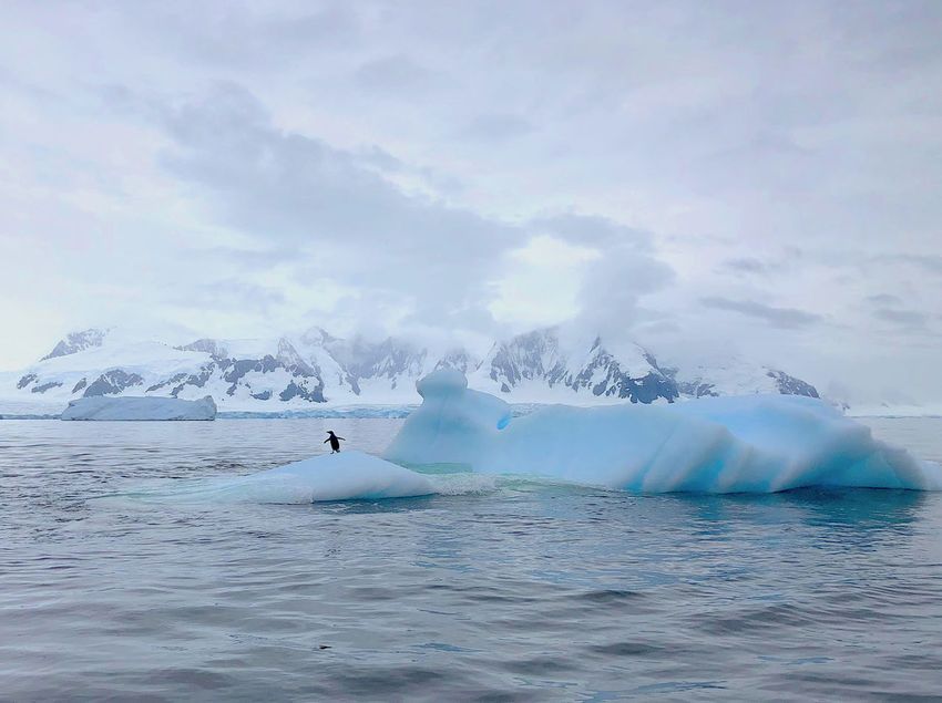
STATE OF THE CLIMATE IN 2019
                          Antarctica and the Southern Ocean
                                                                         Editors

                                                                     Jessica Blunden
                                                                      Derek S. Arndt

                                                                     Chapter Editors

                                                                                                                                                              Downloaded from http://journals.ametsoc.org/bams/article-pdf/101/8/S287/4988921/bamsd200090.pdf by guest on 15 September 2020
                                                                   Peter Bissolli
                                                               Howard J. Diamond
                                                           Matthew L. Druckenmiller
                                                                Robert J. H. Dunn
                                                                Catherine Ganter
                                                                 Nadine Gobron
                                                                  Rick Lumpkin
                                                          Jacqueline A. Richter-Menge
                                                                      Tim Li
                                                               Ademe Mekonnen
                                                              Ahira Sánchez-Lugo
                                                                 Ted A. Scambos
                                                                Carl J. Schreck III
                                                              Sharon Stammerjohn
                                                               Diane M. Stanitski
                                                                 Kate M. Willett

                                                                     Technical Editor

                                                                     Andrea Andersen

                                                    BAMS Special Editor for Climate

                                                                      Richard Rosen

                                                   American Meteorological Society

AU G U S T 2 0 2 0 | S t a t e o f t h e C l i m a t e i n 2 0 1 9                      6 . A N TA R C T I C A A N D T H E S O U T H E R N O C E A N   S288
Cover credit:
Adélie penguin on a floating piece of glacier ice near Jenny Island (a few kilometers from the
British Antarctic Survey base at Rothera) west of the Antarctic Peninsula. The photo was taken
by Ted Scambos on 31 January 2020.

                                                                                                                                             Downloaded from http://journals.ametsoc.org/bams/article-pdf/101/8/S287/4988921/bamsd200090.pdf by guest on 15 September 2020
Antarctica and the Southern Ocean is one chapter from the State of the Climate in 2019
annual report and is available from https://doi.org/10.1175/BAMS-D-20-0090.1. Compiled
by NOAA’s National Centers for Environmental Information, State of the Climate in 2019 is
based on contributions from scientists from around the world. It provides a detailed update
on global climate indicators, notable weather events, and other data collected by environ-
mental monitoring stations and instruments located on land, water, ice, and in space. The
full report is available from https://doi.org/10.1175/2020BAMSStateoftheClimate.1.

How to cite this document:

Citing the complete report:
Blunden, J. and D. S. Arndt, Eds., 2020: State of the Climate in 2019. Bull. Amer. Meteor. Soc.,
101 (8), Si–S429, https://doi.org/10.1175/2020BAMSStateoftheClimate.1.

Citing this chapter:
Scambos, T. and S. Stammerjohn, Eds., 2020: Antarctica and the Southern Ocean
[in “State of the Climate in 2019"]. Bull. Amer. Meteor. Soc., 101 (8), S287–S320,
https://doi.org/10.1175/BAMS-D-20-0090.1.

Citing a section (example):
Reid, P., S. Stammerjohn, R. A. Massom, S. Barreira, T. Scambos, and J. L. Lieser, 2020: Sea ice
extent, concentration, and seasonality [in “State of the Climate in 2019"]. Bull. Amer. Meteor.
Soc., 101 (8), S304–S306, https://doi.org/10.1175/BAMS-D-20-0090.1.

  AU G U S T 2 0 2 0 | S t a t e o f t h e C l i m a t e i n 2 0 1 9   6 . A N TA R C T I C A A N D T H E S O U T H E R N O C E A N   S289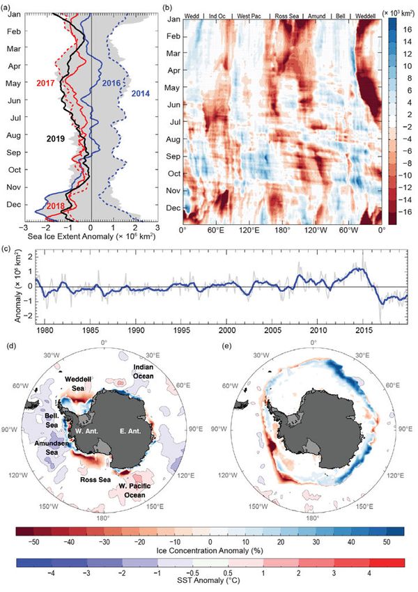
Editor and Author Affiliations (alphabetical by name)
Abrahamsen, E. Povl, Polar Oceans Group, British Antarctic Survey,                    Lieser, Jan L., Bureau of Meteorology, Hobart, Tasmania, Australia, and
    Cambridge, United Kingdom                                                              Institute for Marine and Antarctic Studies, University of Tasmania, Hobart,
Barreira, Sandra, Argentine Naval Hydrographic Service, Buenos Aires,                      Tasmania, Australia
    Argentina                                                                         Liu, Hongxing, Department of Geography, University of Cincinnati, Cincinnati,
Bitz, Cecilia M., Atmospheric Sciences Department, University of Washington,               Ohio
    Seattle, Washington                                                               Long, Craig S., NOAA/NWS National Centers for Environmental Prediction,
Butler, Amy, NOAA/ESRL Chemical Sciences Division, Boulder, Colorado                       College Park, Maryland
Clem, Kyle R., School of Geography, Environment and Earth Sciences, Victoria          Maclennan, Michelle, Department of Atmospheric and Oceanic Sciences,
    University of Wellington, Wellington, New Zealand                                      University of Colorado-Boulder, Boulder, Colorado
Colwell, Steve, British Antarctic Survey, Cambridge, United Kingdom                   Massom, Robert A., Australian Antarctic Division and Australian Antarctic
Coy, Lawrence, Science Systems and Applications, Inc., NASA Goddard Space                  Program Partnership (AAPP), Hobart, Tasmania, Australia
    Flight Center, Greenbelt, Maryland                                                Massonnet, François, Centre de Recherches sur la Terre et le Climat Georges
de Laat, Jos, Royal Netherlands Meteorological Institute (KNMI), DeBilt,                   Lemaître (TECLIM), Earth and Life Institute, Université Catholique de
    Netherlands                                                                            Louvain, Louvain-la-Neuve, Belgium
du Plessis, Marcel D., Department of Marine Science, University of                    Mazloff, Matthew R., Scripps Institution of Oceanography, University of

                                                                                                                                                                          Downloaded from http://journals.ametsoc.org/bams/article-pdf/101/8/S287/4988921/bamsd200090.pdf by guest on 15 September 2020
    Gothenburg, Gothenburg, Sweden and Southern Ocean Carbon and                           California-San Diego, San Diego, California
    Climate Observatory, CSIR, South Africa                                           Mikolajczyk, David, Space Science and Engineering Center, University of
Fogt, Ryan L., Department of Geography, Ohio University, Athens, Ohio                      Wisconsin-Madison, Madison, Wisconsin
Fricker, Helen Amanda, Scripps Institution of Oceanography, University of             Narayanan, A., Indian Institute of Technology, Madras, Chennai, India
    California-San Diego, San Diego, California                                       Nash, Eric R., Science Systems and Applications, Inc., NASA Goddard Space
Fyfe, John, Canadian Centre for Climate Modelling and Analysis, University of              Flight Center, Greenbelt, Maryland
    Victoria, Victoria, British Columbia, Canada                                      Newman, Paul A., NASA Goddard Space Flight Center, Greenbelt, Maryland
Gardner, Alex S., Jet Propulsion Laboratory, California Insitute of Technology,       Petropavlovskikh, Irina, Cooperative Institute for Research in Environmental
    Pasadena, California                                                                   Sciences, University of Colorado Boulder, and NOAA/OAR Earth System
Gille, Sarah T., Scripps Institution of Oceanography, University of California at          Research Laboratory, Boulder, Colorado
    San Diego, La Jolla, California                                                   Pitts, Michael, NASA Langley Research Center, Hampton, Virginia
Gorte, Tessa, Department of Atmospheric and Oceanic Sciences, University of           Queste, Bastien Y., Department of Marine Sciences, University of
    Colorado-Boulder, Boulder, Colorado                                                    Gothenburg, Gothenburg, Sweden
Gregor, L., ETH, Zürich, Switzerland                                                 Reid, Phillip, Australian Bureau of Meteorology and Australian Antarctic
Hobbs, Will, Australian Antarctic Program Partnership and ARC Centre of                    Program Partnership (AAPP), Hobart, Tasmania, Australia
    Excellence for Climate Extremes (CLEX), University of Tasmania, Hobart,           Roquet, F., Department of Marine Sciences, University of Göteborg, Göteborg,
    Tasmania, Australia                                                                    Sweden
Johnson, Bryan, NOAA/OAR Earth System Research Laboratory, Global                     Santee, Michelle L., NASA Jet Propulsion Laboratory, California Institute of
    Monitoring Division, and University of Colorado, Boulder, Colorado                     Technology, Pasadena, California
Keenan, Eric, Department of Atmospheric and Oceanic Sciences, University of           Scambos, Ted A., Earth Science and Observation Center, CIRES, University of
    Colorado-Boulder, Boulder, Colorado                                                    Colorado, Boulder Colorado
Keller, Linda M., Department of Atmospheric and Oceanic Sciences,                     Stammerjohn, Sharon, Institute of Arctic and Alpine Research, University of
    University of Wisconsin-Madison, Madison, Wisconsin                                    Colorado, Boulder, Colorado
Kramarova, Natalya A., NASA Goddard Space Flight Center, Greenbelt,                   Strahan, Susan, Universities Space Research Association, NASA Goddard
    Maryland                                                                               Space Flight Center, Greenbelt, Maryland
Lazzara, Matthew A., Department of Physical Sciences, School of Arts                  Swart, Sebastiann, Department of Marine Sciences, University of
    and Sciences, Madison Area Technical College, and Space Science and                    Gothenburg, Gothenburg, Sweden and Department of Oceanography,
    Engineering Center, University of Wisconsin-Madison, Madison, Wisconsin                University of Cape Town, Rondebosch, South Africa
Lenaerts, Jan T. M., Department of Atmospheric and Oceanic Sciences,                  Wang, Lei, Department of Geography and Anthropology, Louisiana State
    University of Colorado-Boulder, Boulder, Colorado                                     University, Baton Rouge, Louisiana

Editorial and Production Team
Andersen, Andrea, Technical Editor, Innovative Consulting                             Love-Brotak, S. Elizabeth, Lead Graphics Production, NOAA/NESDIS
    Management Services, LLC, NOAA/NESDIS National Centers for                            National Centers for Environmental Information, Asheville, North Carolina
    Environmental Information, Asheville, North Carolina                              Misch, Deborah J., Graphics Support, Innovative Consulting Management
Griffin, Jessicca, Graphics Support, Cooperative Institute for Satellite                  Services, LLC, NOAA/NESDIS National Centers for Environmental
    Earth System Studies, North Carolina State University, Asheville,                     Information, Asheville, North Carolina
    North Carolina                                                                    Riddle, Deborah B., Graphics Support, NOAA/NESDIS National Centers for
Hammer, Gregory, Content Team Lead, Communications and Outreach,                          Environmental Information, Asheville, North Carolina
    NOAA/NESDIS National Centers for Environmental Information,                       Veasey, Sara W., Visual Communications Team Lead, Communications and
    Asheville, North Carolina                                                             Outreach, NOAA/NESDIS National Centers for Environmental Information,
                                                                                          Asheville, North Carolina

                 AU G U S T 2 0 2 0 | S t a t e o f t h e C l i m a t e i n 2 0 1 9                 6 . A N TA R C T I C A A N D T H E S O U T H E R N O C E A N   S290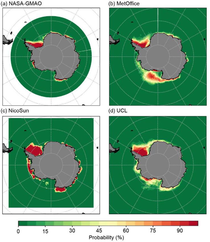
6. Table of Contents

List of authors and affiliations...................................................................................................S290
a. Overview .................................................................................................................................S292
b. Atmospheric circulation and surface observations..............................................................S293
     Sidebar 6.1: The 2019 southern stratospheric warming.....................................................S297
c. Surface mass balance of the ice sheet...................................................................................S298
d. Seasonal melt extent and duration for the ice sheet.......................................................... S300
     Sidebar 6.2: Recent changes in the Antarctic ice sheet.....................................................S302
e. Sea ice extent, concentration, and seasonality................................................................... S304

                                                                                                                                                                   Downloaded from http://journals.ametsoc.org/bams/article-pdf/101/8/S287/4988921/bamsd200090.pdf by guest on 15 September 2020
f. Southern Ocean........................................................................................................................S307
		 1. Variability in the decline of Antarctic bottom water volume..................................S307
		 2. Ocean temperatures on the Antarctic continental shelf from
			animal-borne sensors................................................................................................. S308
		 3. Surface heat fluxes..................................................................................................... S308
		 4. Surface CO2 fluxes.......................................................................................................S310
g. 2019 Antarctic ozone hole......................................................................................................S310
     Sidebar 6.3: Sea Ice Prediction Network-South: coordinating seasonal
     predictions of sea ice for the Southern Ocean................................................................... S313
Acknowledgments.......................................................................................................................S316
Appendix: Acronym List.............................................................................................................. S317
References....................................................................................................................................S318

*Please refer to Chapter 8 (Relevant datasets and sources) for a list of all climate variables and
datasets used in this chapter for analyses, along with their websites for more information and
access to the data.

  AU G U S T 2 0 2 0 | S t a t e o f t h e C l i m a t e i n 2 0 1 9                         6 . A N TA R C T I C A A N D T H E S O U T H E R N O C E A N   S291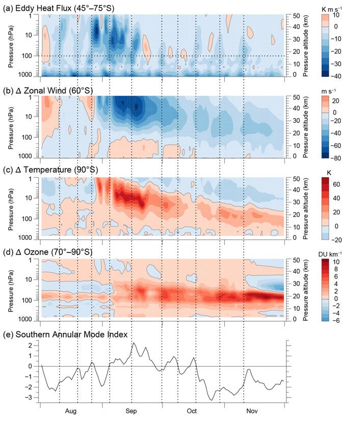
6. ANTARCTICA AND THE SOUTHERN OCEAN
T. Scambos and S. Stammerjohn, Eds.

a. Overview—T. Scambos and S. Stammerjohn
   Antarctica experienced a dramatic stratospheric warming event in early September 2019 that
strongly affected climate patterns in the final four months of the year, and led to the smallest
ozone hole since the early 1980s. The event was caused by a series of upward-propagating tropo-
spheric waves in late August, resulting in above-average temperatures in the stratosphere that
inhibited polar stratospheric cloud formation and greatly reduced ozone loss. In the troposphere,

                                                                                                                                             Downloaded from http://journals.ametsoc.org/bams/article-pdf/101/8/S287/4988921/bamsd200090.pdf by guest on 15 September 2020
the Southern Annular Mode (SAM) was strongly negative in the last three months of the calen-
dar year, reflective of anomalously high pressure conditions south of 60°S and weak westerly
winds. Together, the stratospheric warming in September and related surface conditions start-
ing thereafter contributed to anomalous warm surface spring conditions, setting several high-
temperature records. Meanwhile, anomalously low sea ice extent (below the 1981–2010 mean)
persisted throughout 2019, continuing a succession of negative Antarctic sea ice extent anomalies
since September 2016. The year 2019 was also characterized by warm surface ocean conditions
and large positive net ocean heat flux anomalies (into the ocean) south of 35°S. In contrast, ice
sheet surface mass balance was near normal for the year (compared with 1981–2010), though
with high monthly variability due to variable precipitation, sublimation, and summer surface
melt. However, the ice sheet continued to lose mass in 2019, not due to surface changes but rather
ocean–ice sheet interactions, with the highest rates of mass loss occurring in West Antarctica
and Wilkes Land, East Antarctica.
   The state of Antarctica’s climate, weather, ice, ocean, and ozone in 2019 is presented below. Most
sections compare the 2019 anomalies with the 1981–2010 climatology wherever there are available
data to do so. The ozone section and the sidebar on stratospheric warming compare the 2019 anomaly
to the full record (1980–2019)
when such data are available
to better emphasize how un-
usual stratospheric conditions
were in 2019. We also include
a sidebar on ice sheet changes
this year that reviews ice sheet
and ice shelf trends over the
past three decades. In coming
years, this sidebar topic will
develop into a separate section
detailing annual preliminary
assessments of Antarctica’s
ice mass balance. New sub-
sections on ocean heat uptake
and ocean CO2 uptake are in-
cluded in our Southern Ocean
section. Place names for data
sites or climate events noted
in this chapter are provided
in Fig. 6.1.                          Fig. 6.1. Map of stations and other regions discussed in the chapter.

  AU G U S T 2 0 2 0 | S t a t e o f t h e C l i m a t e i n 2 0 1 9   6 . A N TA R C T I C A A N D T H E S O U T H E R N O C E A N   S292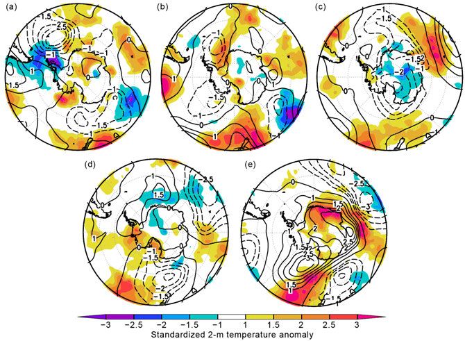
b. Atmospheric circulation and surface observations—K. R. Clem, S. Barreira, R. L. Fogt, S. Colwell,
L. M. Keller, M. A. Lazzara, and D. Mikolajczyk
The stratospheric warming
anomaly in September was the
main circulation feature of 2019
(see Sidebar 6.1), resulting in a
record weak stratospheric vortex,
an earlier-than-normal seasonal
breakdown of the stratospheric
vortex (section 6g), and many
record-setting positive pressure
and temperature anomalies in
the troposphere and surface layer
during October–December. Prior to
Downloaded from http://journals.ametsoc.org/bams/article-pdf/101/8/S287/4988921/bamsd200090.pdf by guest on 15 September 2020
the stratospheric warming event,
the circulation exhibited typical
month-to-month and regional
variability. June was character-
ized by record low temperature
and pressure anomalies across
the continent. For the Antarctic
continent as a whole, 2019 was the
second-warmest year on record
(since 1979), +0.55°C (+2.1 std. dev.)
above the 1981–2010 climatology
(based on reanalysis described be-
low and as presented in Fig. 6.2b).
This surpasses 2018, which is now
the third-warmest year on record.
The warmest year in the record
is 1980. We used the European
Centre for Medium-Range Weather
Forecast (ECMWF) fifth-generation
atmospheric reanalysis (ERA5; Co-
pernicus Climate Change Service
[C3S] 2017) to evaluate atmospheric
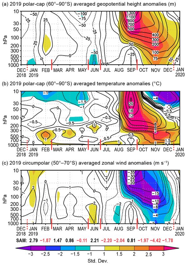
circulation for the year. Figure 6.2
Fig. 6.2. Area-averaged (weighted by cosine of latitude) monthly
shows the monthly geopotential
anomalies over the southern polar region in 2019 relative to 1981–
height (Fig. 6.2a) and temperature 2010. Vertical axes are pressure in hPa. (a) Polar cap (60°–90°S) aver-
(Fig. 6.2b) anomalies averaged over aged geopotential height anomalies (contour interval is 25 m up to
the polar cap (60°–90°S), and the ±100 m, 100 m from ±100 to ±500 m, and 200 m after ±500 m ). (b) Polar
monthly circumpolar zonal wind cap averaged temperature anomalies (contour interval is 0.5°C up to
anomalies (Fig. 6.2c) averaged over ±2°C, 2°C between ±2°C and ±8°C, and 4°C after ±8°C). (c) Circumpolar
50°–70°S. The anomalies are con- (50°–70°S) averaged zonal wind anomalies (contour interval is 2 m s −1
from ±2 m s −1 to ±10 m s −1 and 5 m s −1 after 10 m s −1, with additional
toured, with standard deviations
contour at ±1 m s −1). Shading depicts std. dev. of monthly anomalies
relative to the 1981–2010 monthly
from the 1981–2010 climatological average as indicated by color bar at
climatology overlain as color shad- bottom. (Source: ERA5 reanalysis.) Red vertical bars indicate the five
ing. To investigate the surface climate periods used in Fig. 6.3; the dashed lines near Dec 2018 and
climate anomalies, the year was Dec 2019 indicate circulation anomalies wrapping around the calendar
split into five periods, with the pe- year. Values from the Marshall (2003) SAM index are shown below (c)
riods characterized by differing yet in black (positive values) and red (negative values).
AU G U S T 2 0 2 0 | S t a t e o f t h e C l i m a t e i n 2 0 1 9 6 . A N TA R C T I C A A N D T H E S O U T H E R N O C E A N S293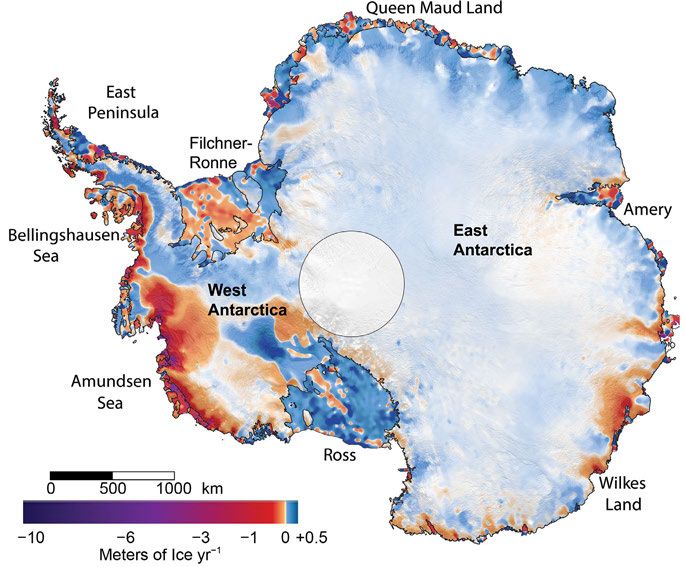
relatively persistent circulation and
temperature anomaly patterns: (1)
January–February, (2) March–May,
(3) June, (4) July–September, and
(5) October–December. Standard-
ized surface pressure (contours)
and temperature (color shaded)
anomalies averaged for each period
relative to the 1981–2010 climatol-
ogy are shown in Fig. 6.3. Monthly
temperature and pressure anoma-
lies from select Antarctic staffed
(Amundsen–Scott, Marambio,
Neumayer, and Syowa) and au-

                                                                                                                                             Downloaded from http://journals.ametsoc.org/bams/article-pdf/101/8/S287/4988921/bamsd200090.pdf by guest on 15 September 2020
tomated (Gill AWS, Relay Station
AWS) weather stations are shown
in Fig. 6.4.
   The year 2019 began with two
                                       Fig. 6.3. Standardized surface pressure (contours) and 2-m temperature
centers of anomalous low pres- (shaded) anomalies relative to 1981–2010 for (a) Jan–Feb 2019; (b) Mar–May
sure during January and February 2019; (c) Jun 2019; (d) Jul–Sep 2019; (e) Oct–Dec 2019. Contour interval is
(Fig. 6.3a), one located in the south- 0.5 std. dev. for surface pressure anomalies with the ±0.5 contour omitted.
west South Pacific (−1.5 std. dev.) Shading represents standard deviation of 2-m temperature anomalies.
and one in the South Atlantic (Source: ERA5 reanalysis.)
(−3 std. dev.). These low-pressure
anomalies produced above-average temperatures on the Ross Ice Shelf and the East Antarctic
Plateau, but below-average temperatures across the Antarctic Peninsula; the polar cap average
mid-tropospheric temperature was +1°C (2 std. dev.) above normal in February (Fig. 6.2b). On the
eastern side of the Plateau, Relay Station AWS (Fig. 6.4e) set a record high monthly mean tempera-
ture for February (−31.7°C, +6.1°C above normal) and a record high monthly mean wind speed
for February (8.2 m s−1, not shown). Monthly mean temperatures on the Antarctic Peninsula (i.e.,
Marambio Station; Fig. 6.4b) were below normal for January and February, but no records were set.
   The austral autumn months (March–May) were relatively quiescent, with pressures and tem-
peratures close to the climatological average across most of the continent (Figs. 6.2, 6.3b). The
exception was over the far southern Atlantic Ocean where low-pressure systems were present
most of the period, resulting in a deep low-pressure anomaly (−1.5 std. dev.) in the Weddell Sea.
This produced above-average temperatures (+2.5 std. dev.) over much of the eastern Weddell
Sea, while another low-pressure anomaly (−1.5 std. dev.) over the eastern Ross Sea advected the
anomalous warm air from the Weddell Sea across interior West Antarctica and onto the Ross Ice
Shelf. The cyclonic conditions in the Weddell Sea dissipated temporarily during March and were
replaced by anomalous high pressure over the southern Atlantic Ocean (not shown). During this
time, Neumayer Station reported a record low monthly mean temperature of −17°C (−4.2°C below
normal) in March (Fig. 6.4c).
   During June, the circulation became quite anomalous. Pressures were generally 1.5–2.5 std. dev.
below normal, temperatures were 1–2 std. dev. below normal across most of the continent
(Fig. 6.3c), and the circumpolar zonal winds in the troposphere were more than 2 m s−1 (1 std. dev.)
above normal (Fig. 6.2c). The station-based Southern Annular Mode (SAM) index (Marshall 2003),
which measures the anomalous pressure gradient between the Southern Hemisphere (SH) middle
latitudes and Antarctica, was strongly positive in June, reaching +2.21 (10th highest for June on
record since 1957). The Ferrell, Marble Point, and Gill AWSs on the Ross Ice Shelf (Fig. 6.4f) as well
as Possession Island AWS in the Ross Sea, all reported record low monthly mean pressures in June
that were 13–14.5 hPa below normal. On the Plateau, Dome C II AWS (631.4 hPa, −16.0 hPa below

  AU G U S T 2 0 2 0 | S t a t e o f t h e C l i m a t e i n 2 0 1 9   6 . A N TA R C T I C A A N D T H E S O U T H E R N O C E A N   S294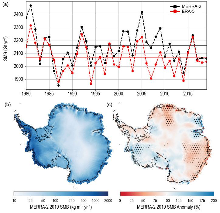
Downloaded from http://journals.ametsoc.org/bams/article-pdf/101/8/S287/4988921/bamsd200090.pdf by guest on 15 September 2020
Fig. 6.4. Monthly Antarctic climate anomalies during 2019 at six representative stations (four staffed
[a]–[d], and two automatic [e]–[f]). Anomalies for temperature (°C) are shown in red and anomalies for
MSLP/surface pressure (hPa) are shown in blue, with filled circles denoting record anomalies for a given
month. Anomalies for the four staffed stations are based on differences from the monthly 1981–2010
averages; for AWS, Gill is based on 1985–2014 averages and Relay Station is based on 1995–2010
averages. Observational data used to calculate record values start in 1957 for Amundsen–Scott and
Syowa, 1970 for Marambio, 1981 for Neumayer, 1985 for Gill AWS, and 1995 for Relay Station AWS.
The surface station data are available online at https://legacy.bas.ac.uk /met /READER /data.html (Turner
et al. 2004) and ftp://amrc.ssec.wisc.edu/pub/aws.

normal); Vostok (612.4 hPa, −11.7 hPa); and Amundsen–Scott (671.0 hPa, −9.8 hPa, Fig. 6.4a) all
had record low monthly mean pressures in June, as did Syowa Station (973.5 hPa, −13.7 hPa) on
the Queen Maud Land coast. Relay Station AWS had very low monthly mean pressure (626.8 hPa,
−9.1 hPa), but no record was set. In contrast to the below-average temperatures and pressures
over the main Antarctic continent, the Antarctic Peninsula experienced slightly negative pressure
anomalies and above-average temperatures in June due to relatively warm west-northwesterly
flow from the Bellingshausen Sea.
   The overall circulation pattern quickly changed during July–September when it became marked
by a weakening of the tropospheric zonal winds (Fig. 6.2c), positive pressure anomalies over
the Antarctic Peninsula, and a very strong negative pressure anomaly (−2.5 std. dev.) south of
New Zealand that stretched poleward into the Ross Sea. Much of the South Pacific experienced

  AU G U S T 2 0 2 0 | S t a t e o f t h e C l i m a t e i n 2 0 1 9   6 . A N TA R C T I C A A N D T H E S O U T H E R N O C E A N   S295
warm, northerly flow that brought positive temperature anomalies over the Ross Ice Shelf and
Marie Byrd Land (Fig. 6.3d). Possession Island AWS observed a record high monthly mean tem-
perature of −11.7°C (+8.6°C above normal) for July. In West Antarctica, Byrd AWS had positive
temperature anomalies of +2.9 and +4.9°C during July and August, respectively. In September,
strong negative pressure anomalies briefly developed at the surface across most of the continent
with a pronounced zonal wave-3 structure (not shown). These pressure anomalies were strongest
over the Ross Ice Shelf where Ferrell (971.6 hPa, −9.8 hPa), Gill (965.1 hPa, −9.8 hPa; Fig. 6.4f),
and Possession Island (966.6 hPa, −8.3 hPa) AWSs all had record low monthly mean pressures
for September. Ferrell also set a record high monthly mean wind speed of 9.5 m s−1 in September
(not shown).
   The most dramatic feature of the 2019 circulation was a record-setting stratospheric warming
event that developed during September (Fig. 6.2; see Sidebar 6.1 for more details). Initially confined
mainly above 300 hPa and averaged poleward of 60°S, this event was marked by strong positive
geopotential height anomalies of up to 1300 m and a positive temperature anomaly of 20°C at

                                                                                                                                             Downloaded from http://journals.ametsoc.org/bams/article-pdf/101/8/S287/4988921/bamsd200090.pdf by guest on 15 September 2020
the 30–20 hPa level. This was associated with a significant weakening of the stratospheric polar
vortex by up to 35 m s−1. All three anomalies in Fig. 6.2 exceeded 3 std. dev. from the climatologi-
cal mean, and at the 30–10 hPa level, all three anomalies were the largest on record in the ERA5
data beginning in 1979.
   The circulation anomalies in the stratosphere progressed downward into the troposphere dur-
ing October–December (Fig. 6.2). In October, higher-than-normal pressures and temperatures at
the surface (Fig. 6.3e) reversed the general trend of the preceding months. The strongest warming
(>3 std. dev.) occurred across Queen Maud Land. Neumayer (−13.2°C, +4.7°C; Fig. 6.4c) and Syowa
(−8.0°C, +5.5°C; Fig. 6.4d) stations, as well as Relay Station AWS (−42.3°C, +7.0°C; Fig. 6.4e), all
set record high temperatures for October, with Neumayer also setting a record high pressure in
November (994.2 hPa, +9.5 hPa). There was a very strong anticyclonic (>3 std. dev.) anomaly over
the Ross Sea region. Marble Point AWS tied its record high pressure for November (982.8 hPa,
+11.0 hPa), while Ferrell, Possession Island, and Gill AWSs (Fig. 6.4f) had near-record high pres-
sure for November (8–11.5 hPa above normal). The SAM index reached its largest negative mean
monthly value of the year in November of −4.42 (second lowest for November on record since
1957). In the Antarctic interior, Relay Station AWS, Amundsen–Scott (Fig. 6.4a), and Vostok sta-
tions all had higher-than-normal pressure for October through December, but no records were
set. In the Weddell Sea region, Halley Station set a record high monthly mean temperature of
−3.1°C (+2.1°C) in December.

  AU G U S T 2 0 2 0 | S t a t e o f t h e C l i m a t e i n 2 0 1 9   6 . A N TA R C T I C A A N D T H E S O U T H E R N O C E A N   S296
Sidebar 6.1: The
2019 southern stratospheric warming—P. NEWMAN, E. R. NASH,
N. KRAMAROVA, A. BUTLER
The Southern Hemisphere (SH) polar strato-
sphere is typically quite cold in the July–
September period with temperatures well be-
low 195 K in the lower stratosphere (~50 hPa).
In September 2019, the southern polar strato-
sphere was disrupted by a sudden warming
event. While warmings are typical in the
Northern Hemisphere (NH), there has been only
one major stratospheric warming observed in
Downloaded from http://journals.ametsoc.org/bams/article-pdf/101/8/S287/4988921/bamsd200090.pdf by guest on 15 September 2020
the SH historical record, in 2002. Warmings are
characterized by a dramatic warm-up of the po-
lar stratosphere, a deceleration of the westerly
polar night jet, and an increase of polar ozone.
Warmings are driven by planetary-scale waves
that propagate from the troposphere into the
stratosphere on a time-scale of a few days.
There were a series of wave events that
drove the changes seen in September and Oc-
tober 2019. Figure SB6.1a shows the 45°–75°S
eddy heat flux (scaled by the square root of
the pressure) from 1000 hPa (near surface) to
1 hPa, determined from MERRA-2 reanalysis
data (Gelaro et al. 2017). The magnitude of the
eddy heat flux is proportional to the vertical
component of the wave activity, with upward
wave events denoted by negative numbers.
Vertical dashed lines are drawn for each of the
eddy heat flux events (or minima) observed
over the August–November period. There are
10 notable events in this period: 10, 19, 26 Fig. SB6.1. Daily averaged zonal-mean MERRA-2 quantities for 1 Aug–30 Nov
2019. (a) Eddy heat flux over 45°–75°S (K m−1 s −1); departures of: (b) 60°S zonal
August; 4, 15, 30 September; 8, 17, 29 October;
wind (m s −1); (c) South Pole temperature (K); and (d) polar cap ozone (DU km−1)
10 November. The peaks of eddy heat flux at from the 1980–2018 mean. (e) Daily SAM index (Marshall 2003). Eddy heat
100 hPa then extend, within a few days, up to flux values (a) are vertically scaled by the square root of pressure. Vertical
higher levels (10–1 hPa) as these waves propa- dashed lines indicate peaks in the strength of the eddy heat flux at 100 hPa,
gate vertically into the middle stratosphere. indicated by the horizontal line in (a).
The wave events strongly decelerated the
polar night jet by depositing easterly momentum in the middle warming cannot be categorized as a major warming. However,
stratosphere. Figure SB6.1b displays the deviation of the zonal this large deceleration was unprecedented for this period in the
wind at 60°S from a daily 1980–2018 climatology. The wave historical record.
events led to large decelerations. At 60°S and 10 hPa, the The 2019 wave events warmed the polar stratosphere by driv-
wind decelerated from 87 m s−1 on 25 August, to 53 m s−1 on ing descending motion in the core of the Antarctic polar vortex.
2 September. This was followed by a deceleration to 26 m s−1 Figure SB6.1c displays the deviation of the temperature at 90°S
on 11 September. By 17 September, the zonal wind at 10 hPa from a daily 1980–2018 climatology, illustrating the warming
−1
had fallen to 11 m s . Because the wind did not reverse to of the polar stratosphere as a result of the wave events. At the
easterlies at 10 hPa (a major warming is defined by a reversal pole, 10-hPa temperature increased from 192 K on 25 August,
of easterly winds at 10 hPa, 60°S), the 2019 August–September to 221 K on 2 September, followed by a warming to 267 K on
AU G U S T 2 0 2 0 | S t a t e o f t h e C l i m a t e i n 2 0 1 9 6 . A N TA R C T I C A A N D T H E S O U T H E R N O C E A N S29711 September. The large warming reversed the 90°–50°S ther- (below the x-axis), showing how the phase and strength of the
mal gradient as of 6 September and was the earliest reversal annular mode are related to the zonal mean wind in the tropo-
in the historical record, even earlier than the September 2002 sphere. The negative phase of the SAM, which is associated with
warming. anomalously hot and dry conditions in eastern Australia (Lim
The wave events also dramatically increased ozone over the et al. 2019), persisted through at least mid-December and may
polar region during the key period of ozone depletion in August have contributed to the extreme wildfire and heat conditions
and September. Figure SB6.1d shows deviations of the ozone observed there during this time.
density from the 1980–2018 climatology in Dobson Units (DU) The series of wave events in August–October 2019 had a
per kilometer. The highest ozone density is found in the lower profound effect on the SH. The 10 wave events were dominated
stratosphere (below 10 hPa). Again, large changes of column by a planetary-scale wave-1 pattern and propagated vertically
ozone are associated with the individual wave events, increasing from the troposphere to the stratosphere. These waves deceler-
ozone well beyond the 1980–2018 average levels for the dates. ated the flow, eroded the polar vortex, warmed the polar region
The downward influence of the stratospheric warming on the (section 6b), and dramatically increased ozone over Antarctica
Downloaded from http://journals.ametsoc.org/bams/article-pdf/101/8/S287/4988921/bamsd200090.pdf by guest on 15 September 2020
Southern Annular Mode (SAM; Lim et al. 2018, 2019) did not (section 6h). While this event was not categorized as a major
appear until mid-October (Fig. SB6.1e), when the SAM index stratospheric sudden warming, it was the largest warming event
went from a positive to a negative value. The SAM variations observed in the August–September record since 1980.
are in reasonable agreement with Fig. SB6.1b and Fig. 6.2c
c. Surface mass balance of the ice sheet—J. Lenaerts, E. Keenan, M. Maclennan and T. Gorte
The grounded portion of the Antarctic Ice Sheet (AIS) is characterized by a frigid continental
climate. Even in peak summer, atmospheric temperatures on the main continent are low enough
to prevent widespread surface melt (section 6d) or liquid precipitation, unlike the Greenland Ice
Sheet (section 5e). With few exceptions (e.g., on the northern Antarctic Peninsula), any meltwater
that is produced refreezes locally in the firn. Meltwater runoff is a negligible component of ice
sheet mass change on the AIS. On the other hand, sublimation is a significant component of AIS
surface mass balance (SMB; Lenaerts and Van Den Broeke 2012; Agosta et al. 2019; Mottram et
al. 2020), especially in summer and in the windy escarpment zones of the ice sheet, where blow-
ing snow occurs frequently (>50% of the time; Palm et al. 2018). By far the dominant contributor
to AIS SMB, with an approximate magnitude of ~2300 Gt yr−1 over the grounded AIS, is solid
precipitation, i.e., snowfall.
Atmospheric reanalysis products are important tools for analyzing AIS SMB and its two domi-
nant components, snowfall and sublimation, in near-real time. Here we use the MERRA-2 at 0.5°
× 0.625° horizontal resolution (Gelaro et al. 2017) and ERA-5 (ERA-Interim’s successor, employing
0.25° horizontal resolution; Copernicus Climate Change Service [C3S] 2017) reanalysis data to
analyze the 2019 AIS SMB, its spatial and seasonal characteristics, and also to compare it to the
climatological record (1981–2010). Based on recent work comparing reanalysis products with in
situ observations on Antarctica, MERRA-2 and ERA-5 stood out as best-performing (Wang et al.
2016; Gossart et al. 2019; Medley and Thomas 2019); however, important biases remain, which are
associated with the relatively low resolution of the reanalysis products and poor/no representa-
tion of important SMB processes (e.g., blowing snow, clear-sky precipitation).
Acknowledging these limitations, we use these two reanalysis products to provide a time se-
ries of (grounded) AIS SMB from 1980 to 2019 (Fig. 6.5a). The 1981–2010 mean SMB is 2159 ± 131
Gt yr−1 in MERRA-2 and 2070 Gt yr−1 ± 113 Gt yr−1 in ERA-5. While both time series show compa-
rable interannual variations, with year-to-year SMB differences of >300 Gt yr−1 between dry and
wet years, neither of the reanalyses suggest a significant long-term trend in SMB (not shown).
Further, although there is apparent better agreement in some periods relative to others, there
is no significant trend in the difference between MERRA-2 and ERA-5 over the entire 1980–2019
period (p = 0.62).
AU G U S T 2 0 2 0 | S t a t e o f t h e C l i m a t e i n 2 0 1 9 6 . A N TA R C T I C A A N D T H E S O U T H E R N O C E A N S298The 2019 SMB total and
SMB anomaly were 2060 Gt
and −99 Gt, respectively, for
MERRA-2, and 2036 Gt and
−34 Gt, respectively, for ERA-
5, thus showing near-normal
conditions for 2019 (compared
with the 1981–2010 climatol-
ogy). Because both reanalysis
datasets produce similar re-
sults, we use MERRA-2 here-
after to focus on spatial and
seasonal characteristics of
the 2019 SMB. As described
Downloaded from http://journals.ametsoc.org/bams/article-pdf/101/8/S287/4988921/bamsd200090.pdf by guest on 15 September 2020
by various studies, AIS SMB is
typically relatively high (>500
mm w.e.) in the coastal areas
of the ice sheet and decreases
sharply from the coast upward
and poleward on the ice sheet;
the same was true for 2019
(Fig. 6.5b) with SMB values
being 125%) in the Amundsen and Bellingshausen glacial basins, thus offsetting part of the dynamic
mass loss that is ongoing in that area (Sidebar 6.2). On the other hand, 2019 SMB was exception-
ally low compared with the climatology (1 std. dev.), while gray shading: std. dev.).
AU G U S T 2 0 2 0 | S t a t e o f t h e C l i m a t e i n 2 0 1 9 6 . A N TA R C T I C A A N D T H E S O U T H E R N O C E A N S299July 2019 had substantially more snowfall than climatology. The December dry anomaly, which
was preceded by a dry November (~60 Gt cumulative snowfall deficit), may have contributed to
early indications of an anomalously high surface melt year for 2019–20 (as mentioned in section
6d and consistent with section 6b). It appears that low snowfall reduced the amount of highly
reflective fresh snow on the surface, which lowered the albedo and enhanced the melt–albedo
feedback effect early in the 2019/20 melt season.
d. Seasonal melt extent and duration for the ice sheet—L. Wang and H. Liu
Surface melt of the Antarctic Ice Sheet (AIS) is largely confined to the coastal region where it
can contribute to surface mass balance (SMB) changes (section 6c). Here, we report on the aus-
tral spring–summer 2018/19 melt season; therefore, this analysis does not include the extensive
melting that occurred later in 2019 in response to widespread warming (section 6b, Figs. 6.2b,
6.3e). Since Antarctica’s melt season extends well into the first few months of the calendar year,
a complete assessment of the more recent austral melt season (2019/20) is not yet available but
Downloaded from http://journals.ametsoc.org/bams/article-pdf/101/8/S287/4988921/bamsd200090.pdf by guest on 15 September 2020
will be highlighted in next year’s annual report.
Surface melt of the AIS can be mapped using satellite passive microwave data obtained from
the Defense Meteorological Satellite Program (DMSP; Zwally and Fiegles 1994). A nearly continu-
ous record of surface melt exists for the period 1978–present from the DMSP satellite series and
earlier Nimbus series satellites. Daily passive microwave brightness temperature observations,
using the 19 GHz channel at horizontal polarization acquired by the Special Sensor Microwave–
Imager Sounder (SSMIS) onboard the DMSP F17 satellite (ascending passes only), were used to
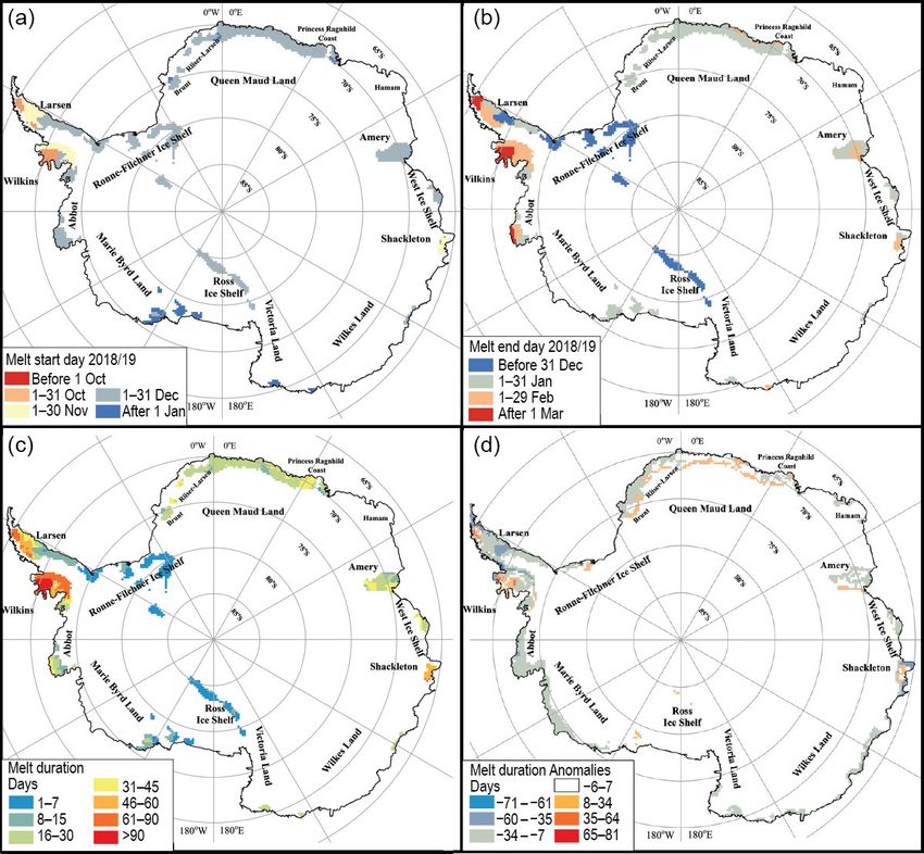
Fig. 6.7. Estimated surface melt for the 2018/19 austral summer: (a) melt start day, (b) melt end
day, (c) melt duration, and (d) melt duration anomalies (day) relative to the 1981–2010 mean.
AU G U S T 2 0 2 0 | S t a t e o f t h e C l i m a t e i n 2 0 1 9 6 . A N TA R C T I C A A N D T H E S O U T H E R N O C E A N S300compute surface melt at a spatial resolution of 25 km. The data were preprocessed and provided
by the U.S. National Snow and Ice Data Center (NSIDC) at level-3 EASE-Grid format (Armstrong
et al. 1994) and were analyzed using a wavelet transform-based edge detection method (Liu et
al. 2005). The wavelet transform detects for every satellite pixel the abrupt change in brightness
temperature when melt first commences and when melt ends (and freezing commences).
Figure 6.7 shows (a) the start day of the melt season and (b) the end day of the melt season
during austral summer 2018/19. The melt duration map shows the total number of melt days at
each grid cell location during the melt season (Fig. 6.7c). The melt anomaly map (Fig. 6.7d) is in
reference to the 30-year mean (1981–2010).
The earliest melt occurred in October 2018 on portions of the Larsen and Wilkins Ice Shelves
(east and west of the Antarctic Peninsula, respectively), which continued into November. Sur-
face melting elsewhere began in November on the Shackleton Ice Shelf in East Antarctica. This
extended to the Queen Maud Land coast and Amery Ice Shelf, with brief events on the Ronne
and Ross Ice Shelves, which ended by late December (Figs. 6.7a,b). Melt events lasted longer on
Downloaded from http://journals.ametsoc.org/bams/article-pdf/101/8/S287/4988921/bamsd200090.pdf by guest on 15 September 2020
the Larsen, Wilkins, and Abbot Ice Shelves, i.e., through February and March of 2019, and on the
Amery and Shackleton Ice Shelves until February 2019 (Fig. 6.7b).
Ice shelves with longer total melt season duration (>45 days; Fig. 6.7c, orange-red color) include
Larsen, Wilkins, and Shackleton (Fig. 6.7c). Areas with moderate melt duration (14–45 days;
Fig. 6.7.c, green-yellow color) include the coast of Queen Maud Land and the Abbot and Amery
Ice Shelves, while sporadic short-term melt (Sidebar 6.2: Recent changes in the Antarctic ice sheet—H. A. FRICKER AND A. S. GARDNER
In recent decades the Antarctic Ice Sheet (AIS) has experi- Observing changes in AIS mass is challenging because it is
enced a rapid increase in grounded ice discharge to the ocean. vast and the signals are small, requiring accurate and consistent
This increase is largely driven by changes in ocean-driven melt- measurements over a wide range of spatial and temporal scales.
ing and ice shelf thinning. Three independent satellite-based techniques are used to es-
The AIS gains mass through snowfall (section 6c) and exports timate AIS mass changes: (a) gravimetry, based on the GRACE
mass primarily via two processes at the margins: iceberg calving and GRACE-FO satellites (e.g., Chen et al. 2009; Velicogna et
(episodic) from the ice fronts and basal melting (continuous) al. 2009, 2020), which directly measure changes in ice sheet
under ice shelves (Lazarra et al. 1999; Depoorter et al. 2013). mass at coarse spatial scale (~300 km) in successive satellite
The net balance between competing mass transfers depends passes, but cannot detect changes in floating ice; (b) mass
on interactions between ice, ocean, and atmosphere. Averaged budget method (MBM), which uses estimates of ice velocity
Downloaded from http://journals.ametsoc.org/bams/article-pdf/101/8/S287/4988921/bamsd200090.pdf by guest on 15 September 2020
over long time scales, the contributions from these mass loss and thickness to determine the amount of solid ice that passes
processes occur in approximate equal proportions (Rignot et across the grounding line and subtracts these against estimates
al. 2013), and their sum offsets the mass gain to maintain AIS of total snow accumulation over the outlet glacier catchments as
in steady state. However, since 1992, many ice shelves have determined from atmospheric reanalyses (Gardner et al. 2018;
experienced net mass loss due to ocean-driven basal melting Rignot et al. 2019); and (c) satellite altimetry using either radar
in excess of the steady state (Adusumilli et al. 2020). after or laser altimeters that measure ice sheet surface elevation
"pushed the ice sheet balance negative" values, which has change over time, combined with model output of changing
pushed the ice sheet mass balance negative The SAM index snow and firn density (that lead to elevation changes without
reached its largest negative mean monthly value of the year in a change in mass) to infer mass changes (e.g., Shepherd et al.
November of −4.42 (2nd lowest for November on record since 2019; Smith et al. 2020).
1957). Major tabular calving events occur on long time scales Satellite radar (since 1992) and laser altimetry (since 2003)
(50–70 years), and since 1992 there have been major calving have provided evidence for widespread elevation loss of outlet
events on several ice shelves: Ross (March and April 2000), glaciers in West Antarctica (Pritchard et al. 2009; Wingham et
Ronne (October 1998, May 2000), Larsen-C (July 2017), Pine al. 1998), particularly in the Amundsen Sea sector (Pritchard
Island (years), and Amery (September 2019). There have also et al. 2012; Shepherd et al. 2001). Soon after the launch of
been several climate change-related collapse events of Antarctic NASA’s GRACE satellites in 2002, these data confirmed that the
Peninsula ice shelves: Larsen A (January 1995), Larsen B (March perimeter of the ice sheet was losing mass (Chen et al. 2009;
2002), and Wilkins (February–July 2008). These are not cyclical, Velicogna 2009) and later revealed evidence of an acceleration
but represent semi-permanent adjustments of ice shelf extent in rates of loss (Velicogna et al. 2014). Early application of the
in light of warmer temperatures and increased melt. MBM (Rignot et al. 2008) confirmed large West Antarctic losses
Fig. SB6.2. Schematic showing relationship between ice shelf buttressing and grounding line flux before (a) and after (b)
the occurrence of ice shelf thinning. (Figure adapted from Gudmundsson et al. 2019.)
AU G U S T 2 0 2 0 | S t a t e o f t h e C l i m a t e i n 2 0 1 9 6 . A N TA R C T I C A A N D T H E S O U T H E R N O C E A N S302that can be largely attributed to accelerated flow of the Pine A recent study (Smith et al. 2020) differenced laser altimetry
Island and Thwaites Glaciers (Gardner et al. 2018; Rignot et al. data from NASA’s ICESat (2003–09) and ICESat-2 (2018–19)
2019). Estimates disagree on the sign of recent mass change laser altimeters to estimate the mass change over Antarctica’s
across East Antarctica, where small changes in net accumulation grounded ice sheet and floating ice shelves from 2003 to 2019.
may greatly impact the net balance (because of its large area). The comparison showed pervasive mass loss in both West
However, the magnitude of the disagreement there is smaller Antarctica and the Antarctic Peninsula, partially offset by mass
than the mass loss signal elsewhere on the ice sheet. gains in East Antarctica; overall, losses outpaced gains, resulting
It can be misleading to directly compare independent pub- in a net grounded ice mass loss of 118 Gt yr−1 for Antarctica (add-
lished estimates from the three techniques, because they are ing a total of 5.2 mm to sea level). In West Antarctica and the
generally made over different time periods. Recognizing this, Antarctic Peninsula, mass loss from the ice shelves accounted
a community Ice-sheet Mass Balance Inter-comparison Experi- for more than 30% of those regions’ total loss, reinforcing the
ment (IMBIE) was established in 2011 to reconcile estimates for notion of a strong link between ice shelf thinning and loss of
1992 to 2011 as part of an assessment of the cryosphere for grounded ice (Fig. SB6.3). The highest ice shelf thinning rates
Downloaded from http://journals.ametsoc.org/bams/article-pdf/101/8/S287/4988921/bamsd200090.pdf by guest on 15 September 2020
the Intergovernmental Panel on Climate Change (IPCC) Fourth were in Thwaites Glacier basin in the Amundsen Sea sector.
Assessment Report. This showed broad agreement among Early analysis of GRACE-FO satellite gravimetry, combined
the three techniques for periods of overlapping measurement with GRACE data, shows reduced acceleration of grounded ice
and concluded that the ice sheet had an overall negative mass loss (i.e., a leveling off) since 2016 (Velicogna et al. 2020). This
−1
balance (71 ± 56 Gt yr ; Shepherd et al. 2012). IMBIE2 (IMBIE leveling off stems from an increase in accumulation in Queen
Team 2018) updated the mass change time series through 2017 Maud Land, George VI land, and the Antarctic Peninsula since
and showed that Antarctica lost mass at an average rate of 109 2016. Glacier losses for the Amundsen Sea sector and Wilkes
± 56 Gt yr−1 between 1992 and 2017. The rates of ice loss from Land were approximately constant since ~2009.
West Antarctica increased by a factor of three (from 53 ± 29 Gt We anticipate that annual assessments of Antarctic mass
yr−1 during 1992–97 to 159 ± 26 Gt yr−1 during 2012–17); from balance will be available for future State of the Climate reports,
the Antarctic Peninsula, the rate increased from 7 ± 13 Gt yr−1 likely derived from NASA’s satellite gravimeter (GRACE-FO) and
to 33 ± 16 Gt yr−1, in part due to accelerated discharge from laser altimeter (ICESat-2).
outlet glaciers after several ice shelf collapse events. IMBIE2
and Shepherd et al. (2019) also showed that
inland thinning is becoming more widespread.
ICESat laser altimetry (2003–08) showed
that elevation changes in grounded ice are
linked to ocean-driven ice shelf thinning
(Pritchard et al. 2009, 2012). The largest thin-
ning rates were observed for coastal West Ant-
arctica, attributed to an enhanced upwelling of
warmer Circumpolar Deep Water (CDW) driven
by increased westerly winds at the continental
shelf break that promoted enhanced melting at
depth near the grounding zone of the largest
glaciers (Thoma et al. 2008; Steig et al. 2012;
Holland et al. 2019). This reduces ice shelf
“buttressing”, i.e., the back-stress that an ice
shelf exerts on the seaward flow of grounded
ice behind it (Thomas 1979; Fig. SB6.2). Sub-
sequent analysis of an 18-year (1994–2012)
altimetry record from four radar altimeter
missions concluded that Antarctic ice shelves
are thinning at an accelerating rate, and that
their volume has declined by 166 ± 48 km3 yr−1 Fig. SB6.3. Mass change of floating and grounded ice (top) from ICESat
between 1994 and 2012 (Paolo et al. 2015). (2003–09) and ICESat-2 (2018–19) data. (Figure adapted from Smith et al. 2020.)
AU G U S T 2 0 2 0 | S t a t e o f t h e C l i m a t e i n 2 0 1 9 6 . A N TA R C T I C A A N D T H E S O U T H E R N O C E A N S303e. Sea ice extent, concentration, and seasonality—P. Reid, S. Stammerjohn, R. A. Massom, S. Barreira,
T. Scambos, and J. L. Lieser
Antarctic sea ice plays a pivotal role in the global climate system. Forming a highly reflective,
dynamic, and insulative blanket that varies seasonally in its areal coverage from ~3 × 10⁶ km2
to ~19–20 × 106 km2, sea ice and its snow cover strongly modifies ocean–atmosphere fluxes and
interaction processes (Bourassa et al. 2013). Moreover, brine rejection into the underlying ocean
during sea ice formation on
some continental shelf ar-
eas leads to the formation
of Antarctic Bottom Water
that contributes to the global
ocean overturning circulation
(Johnson 2008). Antarctic
sea ice also acts as a protec-
Downloaded from http://journals.ametsoc.org/bams/article-pdf/101/8/S287/4988921/bamsd200090.pdf by guest on 15 September 2020
tive buffer for ice shelves
against destructive ocean
swells (Massom et al. 2018)
and modulates the interac-
tion of warm ocean waters
with ice shelf basal cavities
to affect basal melt there
(Timmermann and Hellmer
2013). Finally, it also forms
a key habitat for a myriad of
biota—ranging from micro-
organisms to whales (Thomas
2017)—that are strongly af-
fected by changes in the pres-
ence and seasonal rhythms of
the sea ice cover (e.g., Mas-
som and Stammerjohn 2010).
To place 2019 in context,
net Antarctic sea ice extent
(SIE, the area enclosed by the
ice edge consisting of ≥15%
sea ice concentration [SIC])
showed a slight increasing
trend over 1979–2015 (Comiso
et al. 2016) that was then
marked by increased interan-
nual variability since 2012.
Record high SIE values during
2012–14 (Reid and Massom Fig. 6.9. Antarctic sea ice in 2019. (a) Time series of net SIE anomalies for 2014
2015) were followed by record (dashed blue line), 2016 (solid blue line), 2017 (dashed red line), 2018 (solid
lows from 2016 through 2019 red line), and 2019 (solid black line) (all relative to the 1981–2010 climatology).
(Figs. 6.9a,c). The persistent Gray shading represents the historical range (1979–2018) in SIE anomalies. (b)
Hovmöller (time–longitude) representation of SIE anomalies (× 103 km2 per de-
record-breaking low SIE since
gree of longitude) for 2019. (c) Time series (1979–2019) of monthly average SIE
2016 suggests a response to anomalies (light blue) and their 11-month running mean (dark blue). Maps of
a change in the underlying SIC anomaly (%) and SST anomaly (°C) for (d) Feb and (e) Sep 2019 (all relative
ocean conditions (Meehl et to 1981–2010). Sea ice concentration is based on satellite passive-microwave
al. 2019), particularly for the ice concentration data.
AU G U S T 2 0 2 0 | S t a t e o f t h e C l i m a t e i n 2 0 1 9 6 . A N TA R C T I C A A N D T H E S O U T H E R N O C E A N S304Ross Sea and western Weddell Sea (Fig. 6.9b; Reid et al. 2018, 2019). Also persistent over the last
few years (from mid-2017 through 2019) are positive anomalies in both SIE (e.g., Fig. 6.9a) and
duration (e.g., Fig. 6.10c) in the eastern Amundsen and Bellingshausen Seas (ABS) region. These
persistent positive SIE anomalies could be the result of enhanced sea ice melt (Haumann et al.
2020) together with regional freshening of the upper ocean from observed enhanced melting
of Thwaites Glacier and the adjacent outlet glaciers (Bintanja et al. 2013; St-Laurent et al. 2017).
Below-normal sea surface temperatures (SSTs) were also observed more frequently off the ABS
region since 2017 (e.g., Fig. 6.9d). This region previously showed strong decreases in both sea ice
coverage and duration over 1979–2014 (Fig. 6.10d; Stammerjohn et al. 2015).
Highlights from 2019 include record low monthly mean SIE recorded in both January and June
(Fig. 6.9a), with 59 record low daily values of SIE also occurring in January, May, June, and July.
Indeed, net SIE was below the long-term average (1981–2010) for all days in 2019 (Fig. 6.9c), with
11 days (all in January) also showing the lowest sea ice area (SIA; the actual area covered by sea
ice) on record (not shown). The
Downloaded from http://journals.ametsoc.org/bams/article-pdf/101/8/S287/4988921/bamsd200090.pdf by guest on 15 September 2020
annual daily minimum SIE for
2019 occurred on 28 February (at
2.44 × 10⁶ km2, the seventh lowest
on record), while the daily maxi-
mum was on 30 September (18.46
× 106 km2, 10th lowest on record).
In addition to these highlights,
Antarctic sea ice coverage during
2019 was characterized by high
spatial and seasonal variability,
consistent with variability in
the overlying atmospheric and
underlying oceanic conditions.
The seasonal and regional pro-
gression of SIE anomalies during
the year can be broken into four
phases based on spatio-temporal
analysis (Fig. 6.9b): January–Feb-
ruary; March–June; July–mid-
October; and mid-October–De-
cember. These four phases of SIE
anomaly patterns are described
below, together with associated
atmospheric and/or oceanic fea-
tures drawn from sections 6b and
6g, respectively.
The net circumpolar SIE at the
start of 2019 was at record low
values until about mid-January,
after which the negative net
circumpolar SIE anomaly weak-
ened into mid-February (though
Fig. 6.10. Antarctic sea ice seasonality in 2019. Maps showing 2019 anoma-
remained negative; Fig. 6.9a).
lies of days of (a) advance and (b) retreat, (c) total duration, and (d) dura-
During this time, a distinct and tion trend (following Stammerjohn et al. 2008). Both the climatology (for
persistent zonal wave-3 pattern computing the anomaly) and trend are based on 1981/82–2010/11 data
was observed in the regional SIE (Cavalieri et al. 1996 [updated yearly]), while the 2019/ 20 duration-year
anomalies (Fig. 6.9b), despite a data are from the NASA Team NRTSI dataset (Maslanik and Stroeve 1999).
AU G U S T 2 0 2 0 | S t a t e o f t h e C l i m a t e i n 2 0 1 9 6 . A N TA R C T I C A A N D T H E S O U T H E R N O C E A N S305You can also read