HCLIM38: a flexible regional climate model applicable for different climate zones from coarse to convection-permitting scales
←
→
Page content transcription
If your browser does not render page correctly, please read the page content below
Geosci. Model Dev., 13, 1311–1333, 2020
https://doi.org/10.5194/gmd-13-1311-2020
© Author(s) 2020. This work is distributed under
the Creative Commons Attribution 4.0 License.

HCLIM38: a flexible regional climate model applicable for different
climate zones from coarse to convection-permitting scales
Danijel Belušić1 , Hylke de Vries2 , Andreas Dobler3 , Oskar Landgren3 , Petter Lind1 , David Lindstedt1 ,
Rasmus A. Pedersen4 , Juan Carlos Sánchez-Perrino5 , Erika Toivonen6 , Bert van Ulft2 , Fuxing Wang1 , Ulf Andrae1 ,
Yurii Batrak3 , Erik Kjellström1 , Geert Lenderink2 , Grigory Nikulin1 , Joni-Pekka Pietikäinen6,a ,
Ernesto Rodríguez-Camino5 , Patrick Samuelsson1 , Erik van Meijgaard2 , and Minchao Wu1
1 Swedish  Meteorological and Hydrological Institute (SMHI), Norrköping, Sweden
2 Royal Netherlands Meteorological Institute (KNMI), De Bilt, the Netherlands
3 Norwegian Meteorological Institute (MET Norway), Oslo, Norway
4 Danish Meteorological Institute (DMI), Copenhagen, Denmark
5 Agencia Estatal de Meteorología (AEMET), Madrid, Spain
6 Finnish Meteorological Institute (FMI), Helsinki, Finland
a now at: Climate Service Center Germany (GERICS), Helmholtz-Zentrum Geesthacht, Germany

Correspondence: Danijel Belušić (danijel.belusic@smhi.se)

Received: 24 May 2019 – Discussion started: 15 July 2019
Revised: 12 February 2020 – Accepted: 19 February 2020 – Published: 20 March 2020

Abstract. This paper presents a new version of HCLIM, a          HCLIM cycle has considerable differences in model setup
regional climate modelling system based on the ALADIN–           compared to the NWP version (primarily in the description
HIRLAM numerical weather prediction (NWP) system.                of the surface), it is planned for the next cycle release that the
HCLIM uses atmospheric physics packages from three NWP           two versions will use a very similar setup. This will ensure
model configurations, HARMONIE–AROME, ALARO and                  a feasible and timely climate model development as well as
ALADIN, which are designed for use at different horizon-         updates in the future and provide an evaluation of long-term
tal resolutions. The main focus of HCLIM is convection-          model biases to both NWP and climate model developers.
permitting climate modelling, i.e. developing the climate ver-
sion of HARMONIE–AROME. In HCLIM, the ALADIN
and ALARO configurations are used for coarser resolutions
at which convection needs to be parameterized. Here we de-       1   Introduction
scribe the structure and development of the current recom-
mended HCLIM version, cycle 38. We also present some as-         Regional climate models (RCMs) are currently used at a va-
pects of the model performance.                                  riety of spatial scales and model grid resolutions. Since the
   HCLIM38 is a new system for regional climate modelling,       main motivation of using RCMs is to add value compared
and it is being used in a number of national and international   to global climate models (GCMs) by downscaling over a
projects over different domains and climates ranging from        limited-area domain, the resolution of RCMs is several times
equatorial to polar regions. Our initial evaluation indicates    higher than that of GCMs (e.g. Rummukainen, 2010). The
that HCLIM38 is applicable in different conditions and pro-      added value, expressed as e.g. higher-order statistics, comes
vides satisfactory results without additional region-specific    from the improved resolution of both regional physiogra-
tuning.                                                          phy and atmospheric processes. The GCM resolution is typi-
   HCLIM is developed by a consortium of national meteo-         cally O(100 km), while RCMs use resolutions of O(10 km)
rological institutes in close collaboration with the ALADIN–     (e.g. Taylor et al., 2012; Jacob et al., 2014). At the same
HIRLAM NWP model development. While the current                  time, there is evidence that O(10 km) is too coarse for re-
                                                                 solving some important physical processes and a growing

Published by Copernicus Publications on behalf of the European Geosciences Union.
1312                                                                                                 D. Belušić et al.: HCLIM38

demand for even higher-resolution climate information by           ALADIN–HIRLAM NWP modelling system, and therefore
end users. Building on the development and usage of nu-            this paper focuses on the features that distinguish the climate
merical weather prediction (NWP) and research models at            modelling system from its NWP counterpart. Extensive eval-
resolutions of O(1 km), and with the increase in available         uations of the different HCLIM38 model configurations and
computational resources, climate simulations are increas-          for different regions will be presented in separate studies.
ingly being performed at those very high resolutions (e.g.
Ban et al., 2014; Prein et al., 2015; Kendon et al., 2017; Cop-
pola et al., 2018; Lenderink et al., 2019). An important con-      2     Modelling system description
ceptual change occurs between the resolutions of O(10 km)
and O(1 km), at which the parameterizations of deep con-           2.1    HCLIM structure, terminology and experiment
vection that are used at O(10 km) or coarser resolutions are              setup
typically not employed at O(1 km). The reason for the latter
lies in the fact that the most important deep convection pro-      HCLIM is a regional climate model based on the NWP model
cesses occur at scales of O(1 km) or larger, and therefore the     configuration and scripting system called HARMONIE–
models at those resolutions – also having nonhydrostatic dy-       AROME, which is a part of the ALADIN–HIRLAM (see
namics – should be able to resolve them. Consequently, cli-        Table 1) NWP modelling system (Lindstedt et al., 2015;
mate models at resolutions of O(1 km) are often referred to as     Bengtsson et al., 2017; Termonia et al., 2018). ALADIN–
convection-permitting regional climate models (CPRCMs).            HIRLAM is a limited-area model based on the code that
This still leaves a subset of smaller-scale convection fea-        is shared with the global models IFS and ARPEGE. The
tures that need to be parameterized, which is usually done         ALADIN–HIRLAM model consists of four configurations,
using a shallow convection parameterization. An alternative        namely ALADIN, ALARO, AROME and HARMONIE–
approach is to use scale-aware convection parameterizations        AROME (Table 1). HARMONIE is a scripting system de-
that can adjust their effects based on the fraction of resolved    veloped and used by HIRLAM countries for operational
convection in a model grid box (e.g. Gerard et al., 2009). De-     NWP applications. All the above-mentioned ALADIN–
spite the extensive experience with such modelling systems         HIRLAM model configurations are available in the HAR-
for NWP and research purposes, there are additional concep-        MONIE scripting system, but only the specific configuration
tual and computational challenges when climate simulations         of AROME (HARMONIE–AROME) is officially supported,
are considered. Here we present the new version (cycle 38)         developed and used in HIRLAM NWP applications (Bengts-
of the HARMONIE-Climate (HCLIM hereafter; Lindstedt                son et al., 2017).
et al., 2015; Lind et al., 2016) modelling system, aimed at re-       The HCLIM climate model development is based on
gional climate simulations on convection-permitting scales.        the HARMONIE system. The HARMONIE–AROME model
Because the step from GCM to CPRCM resolution is still             configuration is designed for convection-permitting scales
too large for direct nesting (e.g. Matte et al., 2017), there is   and is used with nonhydrostatic dynamics, which is the pri-
a need for an intermediate model grid between GCMs and             mary focus of HCLIM development. The model configura-
CPRCMs. HCLIM has options for this as described below.             tions ALADIN and ALARO are also used in HCLIM appli-
   HCLIM cycle 38 (HCLIM38) has been developed and                 cations, typically for coarser resolutions with hydrostatic dy-
maintained by a subset of national meteorological insti-           namics. Since HCLIM includes these three different model
tutes from the HIRLAM consortium: AEMET (Spain),                   configurations, it is necessary to specify which configuration
DMI (Denmark), FMI (Finland), KNMI (the Netherlands),              is used for a given application. Together with specifying the
MET Norway and SMHI (Sweden). HCLIM38 is the new                   cycle used (cycle 38 in this paper), this results in the final ter-
recommended version with considerable changes and im-              minology that is used in these projects: HCLIM38-AROME,
provements compared to the older versions. It is cur-              HCLIM38-ALADIN or HCLIM38-ALARO.
rently being used in a number of projects, some of                    As seen above, HCLIM versions are called cycles to re-
which are large collaborative activities (e.g. the H2020           main consistent with the NWP model configurations. The
European Climate Prediction system – EUCP, https://                cycle numbering of model versions is inherited from the
www.eucp-project.eu/, last access: 18 March 2020; the              ECMWF, who are the first in the chain of model releases
CORDEX Flagship Pilot Study (FPS) on convection (Cop-              (e.g. Bauer et al., 2013). There are 26 countries in Europe
pola et al., 2018); the ELVIC CORDEX FPS on climate                who base their operational NWP on the ALADIN–HIRLAM
extremes in the Lake Victoria Basin, http://www.cordex.            system, although with different configurations and flavours
org/endorsed-flagship-pilot-studies/, last access: 18 March        (e.g. Bengtsson et al., 2017; Termonia et al., 2018; Frogner
2020).                                                             et al., 2019). The HCLIM community strives to keep up with
   The purpose of this paper is to describe the HCLIM38            the NWP cycle releases, but due to the different timescales
modelling system and the available model configurations, as        and applications of climate simulations, the smaller devel-
well as to provide initial insight into some aspects of their      opment community, and other various reasons there can be
performance. HCLIM38 is closely related to the documented          skipped cycles, so gaps in cycles are expected in HCLIM ter-

Geosci. Model Dev., 13, 1311–1333, 2020                                               www.geosci-model-dev.net/13/1311/2020/
D. Belušić et al.: HCLIM38                                                                                                     1313

Table 1. List of main acronyms related to the HCLIM system.

      Acronym       Full name                         Notes
      HIRLAM        High Resolution Limited Area      Collaboration between 10 national meteorological services (Bengtsson et al.,
                    Model                             2017); also the name of the limited-area model which is being phased out and
                                                      has been replaced with the HIRLAM-ALADIN NWP model, in particular with
                                                      the HARMONIE–AROME configuration
      ALADIN        Aire Limitée Adaptation           Collaboration between 16 national meteorological services; also the name of
                    Dynamique Développement           the limited-area model using ARPEGE physics (Termonia et al., 2018)
                    International
      HARMONIE      HIRLAM–ALADIN Research on         The HARMONIE NWP system consists of the HIRLAM-specific AROME
                    Mesoscale Operational NWP in      model configuration (Bengtsson et al., 2017), together with a scripting sys-
                    Euromed                           tem and set of tools for building, running, and validating and verifying the
                                                      HARMONIE–AROME model
      ARPEGE        Action de Recherche Petite        Global model developed at Météo-France (Courtier et al., 1991)
                    Échelle Grande Échelle
      IFS           Integrated Forecasting System     Global model developed at the European Centre for Medium-Range Weather
                                                      Forecasts (ECMWF; Bauer et al., 2013)
      AROME         Applications of Research to       Convection-permitting model developed at Météo-France with HIRLAM
                    Operations at Mesoscale           contributions (Seity et al., 2011; Bengtsson et al., 2017)
      ALARO         ALADIN–AROME                      Limited-area model applicable also in the convection “grey zone”
                                                      (Termonia et al., 2018)
      SURFEX        Surface Externalisée              Surface scheme shared by all HCLIM model configurations
                                                      (Masson et al., 2013)

minology. For example, the HCLIM release before cycle 38            namics are described in Bengtsson et al. (2017) and Ter-
that was described in detail was cycle 36 (Lindstedt et al.,        monia et al. (2018). The three different model configura-
2015), and the next target cycle is 43.                             tions available in HCLIM are designed for different spa-
   The current and historical versions of the code are              tial resolutions (Fig. 1). A comprehensive description of the
archived using Apache Subversion (SVN; https://subversion.          HARMONIE–AROME physics and NWP setup is presented
apache.org/, last access: 18 March 2020), thus providing            in Bengtsson et al. (2017). Consequently, we report only
access to a specific code revision at any time. Code re-            the main features and the differences between HCLIM38-
vision numbers for model experiments are stored in their            AROME and the HARMONIE–AROME NWP system. The
home directory. The model documentation for each cycle              other two configurations, ALADIN and ALARO, are detailed
is archived at the HIRLAM website (https://hirlam.org/trac/         in Termonia et al. (2018), and here we describe the differ-
wiki/HarmonieSystemDocumentation, last access: 18 March             ences in HCLIM38. It is important to note that Bengtsson
2020), which is accessible to registered users. Configura-          et al. (2017) describe the canonical model configurations for
tion information for the experiments analysed here can be           HARMONIE–AROME, and Termonia et al. (2018) describe
found in the Supplement. The domain definition file (Har-           those for ALADIN and ALARO. Canonical model configu-
monie_domains.pm) together with a configuration file (con-          rations form a subset of all possible configurations, which
fig_exp.h) include all information about an experiment setup.       is thoroughly validated for use in a certain NWP context.
The options used to modify the configuration file for the dif-      The configurations presented here differ from the canonical
ferent experiments are listed in Table S1 in the Supplement.        model configurations. One important difference is the sur-
                                                                    face model, which is shared between all the three HCLIM
2.2    HCLIM model configurations                                   model configurations. It is based on the surface model SUR-
                                                                    FEX (Surface Externalisée), with different options activated
                                                                    for climate applications compared to the NWP setup as de-
Unlike the majority of limited-area models, a common char-
                                                                    scribed below.
acteristic of all model configurations in the HCLIM system
is that they use a bi-spectral representation for most prog-
nostic variables, with semi-implicit time integration and a
semi-Lagrangian advection scheme. The details of the dy-

www.geosci-model-dev.net/13/1311/2020/                                                 Geosci. Model Dev., 13, 1311–1333, 2020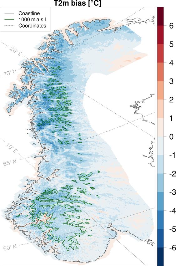
1314                                                                                                  D. Belušić et al.: HCLIM38

                                                                     from a climatology of lake profiles which vary over time and
                                                                     space. HCLIM38 implements the same SICE model as in the
                                                                     NWP setup to simulate the sea ice temperature. The differ-
                                                                     ence in HCLIM38 is that the sea surface temperature and sea
                                                                     ice concentration are updated together with the lateral bound-
                                                                     aries to capture their long-term variation. The urban tile is pa-
                                                                     rameterized by the Town Energy Balance model (TEB; Mas-
                                                                     son, 2000), which is used only at convection-permitting res-
                                                                     olutions.
                                                                        The land cover and soil properties are obtained from
                                                                     the ECOCLIMAP version 2.2 database at 1 km resolution
Figure 1. Intended horizontal grid resolutions for the three model
                                                                     (Faroux et al., 2013) and the Food and Agriculture Organi-
configurations available in HCLIM38 (based on Termonia et al.,
2018).
                                                                     zation database (FAO, 2006), respectively. SURFEX is fully
                                                                     coupled to the atmospheric model, receiving atmospheric
                                                                     forcing over each patch and tile and returning grid-averaged
                                                                     values (heat and momentum fluxes, etc.).
2.2.1   SURFEX
                                                                     2.2.2   ALADIN
SURFEX is an externalized surface modelling system that
parameterizes all components of the surface (Masson et al.,          ALADIN is the default choice in HCLIM38 for simulations
2013). It uses a tiling approach to represent subgrid surface        with grid spacing close to or larger than 10 km. It is the
heterogeneity, with the surface split into four tiles: conti-        limited-area version of the global model ARPEGE, from
nental natural surfaces, sea, inland water and urban areas.          which it inherits all dynamics and physics options. The ver-
The SURFEX tiling approach assumes that the interaction              sion of ALADIN available in HCLIM38 corresponds to the
of each surface tile with the overlying atmosphere is com-           one used in NWP, with the dynamics and physics options
pletely independent of the other tiles present in the grid box.      listed in Table 3 and described in Termonia et al. (2018).
Continental natural surfaces are further divided into subtiles       The difference in HCLIM38 is only in the surface parame-
or patches, accounting for different vegetation characteristics      terizations, which are more suitable for climate simulations
within a grid box. The number of patches can be chosen be-           as described above. HCLIM38-ALADIN is predominantly
tween 1 and 12, but for simplicity it is typically set to 2 in       used as a hydrostatic model with a convection parameteri-
HCLIM38, representing open land and forest.                          zation, so it is not envisaged for use at grid spacings much
   The NWP setup of HARMONIE–AROME (Bengtsson                        smaller than 10 km. Therefore, there is a gap, usually termed
et al., 2017) uses simplified surface processes like the force-      “the grey zone” for convection, between the grid spacing of
restore approach in the soil (Boone et al., 1999) and the com-       10 km and the convection-permitting scales with grid spacing
posite snow scheme by Douville et al. (1995). Such simpli-           smaller than 4 km. HCLIM38 simulations with grid spacing
fied physics are appropriate for short timescales in combina-        within the grey zone should be avoided if possible.
tion with surface data assimilation, but for climate timescales
more sophisticated surface physics are required that can rep-        2.2.3   ALARO
resent e.g. long soil memory and proper snow characteristics.
The default SURFEX version in HCLIM38 was 7.2 (Masson                ALARO has been designed to also operate in the convec-
et al., 2013). However, the state of the more sophisticated          tion grey zone (Fig. 1; Termonia et al., 2018). Unlike tradi-
surface physics options in v7.2 was not considered to be ad-         tional moist convection parameterizations, the Modular Mul-
equate for HCLIM purposes. Therefore, a stepwise upgrade             tiscale Microphysics and Transport scheme (3MT; Gerard
of SURFEX was performed. First, v7.2 was replaced by v7.3,           et al., 2009) addresses the fact that the size of convective
and then the land-surface physics scheme in v7.3 (ISBA) was          cells becomes significant compared to the model grid spac-
replaced by the corresponding scheme from v8.1. The list of          ing as the resolution increases. This allows for great flexi-
SURFEX parameterizations and the related references used             bility in applying the model, which is highly desirable in cli-
in HCLIM38 is given in Table 2. These include e.g. the ISBA          mate applications. Therefore, ALARO was the default choice
multi-layer soil diffusion option (ISBA-DIF) with soil or-           in HCLIM36 (Lindstedt et al., 2015). However, the cou-
ganic carbon taken into account and a 12-layer explicit snow         pling of ALARO with SURFEX as used in HCLIM38 re-
scheme (ISBA-ES). For a proper simulation of temperature             sulted in evaporation from oceans that is too weak in low lat-
in deep and large lakes the inland water (rivers and lakes in-       itudes, causing considerable underestimation of atmospheric
cluding any ice cover) is simulated by FLake. In HCLIM38,            moisture content and consequently a lack of precipitation
FLake uses the lake depth obtained from the Global Lake              in long climate simulations. Similar issues have not been
Data Base (GLDB; Kourzeneva et al., 2012) and is initialized         observed at high latitudes (Toivonen et al., 2019), imply-

Geosci. Model Dev., 13, 1311–1333, 2020                                                www.geosci-model-dev.net/13/1311/2020/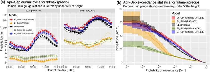
D. Belušić et al.: HCLIM38                                                                                                    1315

Table 2. SURFEX parameterizations used in HCLIM38.

               Model component      Parameterization                                 References
               Sea and ocean        Exchange Coefficients from Unified               Belamari (2005) and
                                    Multi-campaigns Estimates (ECUME)                Belamari and Pirani (2007)
               Sea ice              Simple ICE (SICE)                                Batrak et al. (2018)
               Soil                 ISBA-DIF explicit multi-layer scheme             Boone (2000) and
                                    (14 layers to 12 m of depth)                     Decharme et al. (2011)
               Vegetation and       Jarvis-based stomatal resistance; soil organic   Noilhan and Planton (1989) and
               carbon-related       carbon for soil thermal and hydrological         Decharme et al. (2016)
               processes            properties
               Subgrid hydrology    Subgrid runoff, Horton runoff                    Dümenil and Todini (1992) and
                                                                                     Decharme and Douville (2006)
               Snow                 ISBA-ES explicit snow scheme (12 layers)         Boone and Etchevers (2001) and
                                                                                     Decharme et al. (2016)
               Town                 Town Energy Balance (TEB)                        Masson (2000)
               Inland water         Freshwater lake model (FLake)                    Mironov et al. (2010)

ing that ALARO can be used there. However, it is not the              tions, which are generally considered grid spacings smaller
default option in HCLIM38 because the modelling system                than 4 km. This implies that for downscaling low-resolution
should be applicable at all latitudes. The detailed ALARO             GCMs, it is currently not possible to use the same model con-
description in Termonia et al. (2018) refers to a newer version       figuration at intermediate scales of O(10 km) and convection-
called ALARO1. HCLIM38 uses an older version, ALARO0,                 permitting scales of O(1 km). As described above, the inter-
with some updates from a development version of ALARO1                mediate scales in the current setup are typically simulated
and as such does not correspond to any canonical model                by HCLIM38-ALADIN. This is the preferred option because
configuration. Specifically, in HCLIM38-ALARO the radi-               the two model configurations share the same surface model.
ation scheme ACRANEB from ALARO0 was replaced by                      In this case the soil state in HCLIM38-AROME is initial-
an early version of ACRANEB2 used in ALARO1. Since                    ized in a consistent way, the only difference being the resolu-
it is based on ALARO0, HCLIM38-ALARO still uses the                   tion change. This could help decrease the soil spin-up time,
pseudo-prognostic turbulent kinetic energy (pTKE) turbu-              which is typically 1 year, provided that the precipitation cli-
lence scheme (Geleyn et al., 2006), which has been replaced           matology is similar between the two model configurations.
by TOUCANS (Ďurán et al., 2014) in ALARO1. At the same               However, HCLIM38-AROME can also be used with other
time, HCLIM38-ALARO is coupled to SURFEX, making                      climate models at the lateral boundaries.
this configuration different from the NWP model configura-               HCLIM38-AROME uses a shallow convection parameter-
tion. The full list of used parameterizations and references is       ization based on the eddy diffusivity mass-flux framework
given in Table 3.                                                     (EDMFm; de Rooy and Siebesma, 2008; Bengtsson et al.,
                                                                      2017). The default choice for the turbulence parameteriza-
2.2.4   AROME                                                         tion is the scheme called HARMONIE with RACMO Turbu-
                                                                      lence (HARATU; Lenderink and Holtslag, 2004; Bengtsson
HCLIM38-AROME is a nonhydrostatic CPRCM based on                      et al., 2017), even though the CBR scheme (Cuxart et al.,
the HARMONIE–AROME NWP model configuration (Ta-                       2000) with the diagnostic mixing length from Bougeault and
ble 3), but with different surface model options that are more        Lacarrere (1989) is available as well. HARATU and CBR
suitable for climate applications as described above. It is           mostly differ in the formulation of length scales and values
the recommended option in HCLIM38 for simulations at                  of constants (Bengtsson et al., 2017). A one-moment mi-
convection-permitting scales. AROME is the main focus of              crophysics scheme, ICE3 (Pinty and Jabouille, 1998; Las-
HCLIM development due to the recognized need of the par-              caux et al., 2006), is used, with additional modifications
ticipating institutes for a CPRCM. As such, it is becoming            for cold conditions called OCND2 (Müller et al., 2017).
the backbone of convection-permitting regional climate pro-           The cloud fraction is determined using a statistical scheme
jections for a number of European countries.                          (Bechtold et al., 1995). Similarly to ALADIN, the radia-
   There is no deep convection parameterization in AROME,             tion scheme is a simplified version of the scheme used at
so it can only be used at convection-permitting resolu-

www.geosci-model-dev.net/13/1311/2020/                                                  Geosci. Model Dev., 13, 1311–1333, 2020
1316                                                                                                     D. Belušić et al.: HCLIM38

Table 3. Parameterizations and dynamics of the three model configurations as used in HCLIM38.

  Parameterization   ALADIN                                 ALARO                                  AROME
  and dynamics
  Dynamics           Hydrostatic (Temperton et al., 2001)   Hydrostatic (Temperton et al., 2001)   Nonhydrostatic (Bénard et al., 2010)
  Radiation          RRTM_LW, SW6 (Mlawer et al.,           ACRANEB2 (Mašek et al., 2016;          RRTM_LW, SW6 (Mlawer et al.,
                     1997; Iacono et al., 2008; Fouquart    Geleyn et al., 2017)                   1997; Iacono et al., 2008; Fouquart
                     and Bonnel, 1980)                                                             and Bonnel, 1980)
  Turbulence         CBR (Cuxart et al., 2000); mixing      pTKE (Geleyn et al., 2006)             HARATU (Lenderink and Holtslag,
                     length from Bougeault and Lacar-                                              2004; Bengtsson et al., 2017)
                     rere (1989)
  Microphysics       Lopez (2002); Bouteloup et al.         Lopez (2002)                           ICE3-OCND2 (Pinty and Jabouille,
                     (2005)                                                                        1998; Müller et al., 2017)
  Shallow            KFB (Bechtold et al., 2001; Bazile     Pseudo shallow convection parame-      EDMFm (de Rooy and Siebesma,
  convection         et al., 2012)                          terization (Geleyn, 1987)              2008; Bengtsson et al., 2017)
  Deep convection    Bougeault (1985)                       3MT (Gerard et al., 2009)              –
  Clouds             Smith (1990)                           Xu and Randall (1996)                  Bechtold et al. (1995)
  Orographic         Catry et al. (2008)                    Catry et al. (2008)                    –
  wave drag

the ECMWF, described in Mascart and Bougeault (2011).                  ing that when CNRM-ALADIN is coupled with other com-
The six-spectral-band shortwave radiation (SW6) is based               ponents of the Earth system, such as aerosols (Drugé et al.,
on Fouquart and Bonnel (1980). A rapid radiative transfer              2019), oceans and rivers (Sevault et al., 2014; Darmaraki
model (RRTM) with 16 spectral bands is used for longwave               et al., 2019), the model is called CNRM-RCSM (regional cli-
radiation (Mlawer et al., 1997; Iacono et al., 2008). Monthly          mate system model) even if the schemes for the atmosphere
aerosol climatologies are provided by Tegen et al. (1997).             are the same as described above.
                                                                          The CNRM-AROME41t1 model is currently used for cli-
2.3    Differences from Météo-France–CNRM climate                      mate research (Coppola et al., 2018). This latest version 41t1
       models                                                          uses cycle 41 of AROME, which is described in Termonia
                                                                       et al. (2018) for the NWP system, while the previous cli-
Since the names and model configurations are similar for               mate version was based on cycle 38 (e.g. Fumière et al.,
HCLIM and Météo-France–CNRM climate models (CNRM-                      2019). The differences from HCLIM38-AROME are as fol-
ALADIN and CNRM-AROME), we briefly describe some                       lows. The ICE3 scheme is used for microphysics without the
of the main differences between the latest versions of the             OCND2 modification, and the PMMC09 scheme is used for
HCLIM and CNRM models (see Table 3 for the parameteri-                 shallow convection (Pergaud et al., 2009). Parameterizations
zation schemes used in HCLIM38).                                       by Pergaud et al. (2009) are also used for clouds in addi-
   CNRM-ALADIN has been used in climate mode for more                  tion to Bechtold et al. (1995), which is used in HCLIM38-
than 10 years (e.g. Radu et al., 2008; Colin et al., 2010).            AROME. The surface scheme is version 7.3 of SURFEX
The latest version of ALADIN-Climate, version 6.3 (CNRM-               (Masson et al., 2013). In addition, CNRM-AROME41t1 in-
ALADIN63; Daniel et al., 2019), differs from HCLIM38-                  cludes the COMAD correction for overestimated precipita-
ALADIN in certain physical parameterizations. Firstly, the             tion and unrealistic divergent winds in the vicinity of con-
parameterizations for convection and clouds are different:             vective clouds (Malardel and Ricard, 2015).
CNRM-ALADIN63 includes a Prognostic Condensates Mi-
crophysics and Transport (PCMT) scheme (Piriou et al.,
                                                                       2.4   Differences from HCLIM36
2007; Guérémy, 2011) for dry, shallow and deep convection,
as well as a cloud scheme based on probability distribution
functions (PDFs) by Ricard and Royer (1993). Orographic                The version of the latest operational HCLIM was cycle 36,
wave drag is parameterized by Déqué et al. (1994) along with           described thoroughly by Lindstedt et al. (2015). In the new
Catry et al. (2008), which is used in HCLIM38-ALADIN. A                version, cycle 38, the model system has undergone consid-
climate version of SURFEX 8 (Decharme et al., 2019) is used            erable changes in the parameterizations, physical packages
as the land-surface modelling platform. It is also worth not-          used and target resolutions. The main differences are briefly

Geosci. Model Dev., 13, 1311–1333, 2020                                                  www.geosci-model-dev.net/13/1311/2020/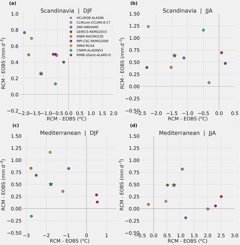
D. Belušić et al.: HCLIM38                                                                                                     1317

described here for easier distinction between the different cy-
cles.
   In HCLIM38, ALADIN is the default model configuration
that should be used for coarser-resolution applications and as
the intermediate model when the target horizontal grid size
is on the kilometre scale or below. In the previous cycles the
default configuration was ALARO. The other main differ-
ence is the update of the surface modelling platform going
from SURFEX v5 to a blend of SURFEX v7 and v8 in order
to improve and enable more accurate land-related processes.
The main improvements in SURFEX processes in cycle 38
are summarized in the following. Similarly to the differences
from the current NWP configuration (see Sect. 2.2.1), a 14-
layer soil diffusion scheme together with a 12-layer explicit
snow scheme are activated, with soil organic carbon taken
into account. The inland water is simulated by the lake model
FLake. The sea ice model SICE is employed for oceans, and
it uses updated sea ice concentrations and sea surface tem-
peratures with the same frequency as the lateral boundaries.
The combined effects from the differences in model configu-
rations lead to considerable improvement in the overall per-
formance. For instance, the near-surface temperature is much
                                                                  Figure 2. Difference between RCMs and E-OBS of near-surface
closer to observations (Fig. S1a in the Supplement), mainly
                                                                  temperature (x axis) and daily precipitation (y axis) for (a, c) DJF
dependent on the utilization of the diffusion soil scheme to-     and (b, d) JJA averaged over 1999–2008 for two PRUDENCE Eu-
gether with the sea ice model. Also, the general precipita-       ropean subregions: (a, b) Scandinavia and (c, d) the Mediterranean.
tion pattern is largely improved, especially during the sum-
mer when the old configuration suffered from a very dry
bias in eastern Europe (Fig. S1b). The smaller temperature        3.1     Performance over European domains
biases can be related to smaller biases generally also found
for radiation and surface heat fluxes in the new configuration    3.1.1    Pan-Europe
(Fig. S2; regions defined in Lindstedt et al., 2015).
                                                                  Here, HCLIM38 is compared to other state-of-the-art RCMs
                                                                  over Europe (Kotlarski et al., 2014). HCLIM38-ALADIN
3   Model performance                                             has been run with a couple of domain configurations sim-
                                                                  ilar to the EURO-CORDEX domain with a horizontal grid
The three configurations of HCLIM38 have been used over
                                                                  spacing of 12 km (EURO-CORDEX uses 0.11◦ resolution;
several different regions and climates. Since HCLIM38-
                                                                  Kotlarski et al., 2014). The boundary conditions were taken
ALADIN is a limited-area version of the global model
                                                                  from the ERA-Interim reanalysis (Dee et al., 2011). Dif-
ARPEGE, the expectation is that it can be used in principle
                                                                  ferences in daily mean near-surface air temperature (T2m)
for any region on Earth. Consequently, the model is not tuned
                                                                  and precipitation between nine RCMs (including HCLIM38-
for specific regions. HCLIM38-ALARO has mostly been
                                                                  ALADIN) and E-OBS version 17 gridded observations (Hay-
used in high latitudes where it performs well. HCLIM38-
                                                                  lock et al., 2008) were calculated for the Prediction of Re-
AROME has been successfully used on domains ranging
                                                                  gional scenarios and Uncertainties for Defining European
from the tropics and different mid-latitude regions to the Arc-
                                                                  Climate change risks and Effects (PRUDENCE) regions in
tic, indicating that it can be used for various climates with-
                                                                  Europe (Christensen and Christensen, 2007) based on a com-
out additional modifications. Here we illustrate the capabil-
                                                                  mon 10-year period (1999–2008). RCMs were interpolated
ity and performance of HCLIM38 with a number of selected
                                                                  to the E-OBS 0.25◦ regular grid prior to comparison. Figure
examples for different domains and model configurations.
                                                                  2 shows the results for the winter (DJF) and summer (JJA)
More in-depth evaluation studies are left for separate papers
                                                                  seasons for the Scandinavia and Mediterranean regions. The
for each of the domains analysed below as well as for other
                                                                  results for these two regions, which are representative for
domains (e.g. Crespi et al., 2019; Toivonen et al., 2019; Wu
                                                                  most PRUDENCE regions, show that HCLIM38-ALADIN
et al., 2019). The model experiments are summarized in Ta-
                                                                  is generally colder and wetter than E-OBS. However, it can
ble S1.
                                                                  be seen that most of the other RCMs are also wetter than
                                                                  E-OBS and that HCLIM38-ALADIN is generally in close
                                                                  agreement with E-OBS in winter (Fig. S1). Larger differ-

www.geosci-model-dev.net/13/1311/2020/                                               Geosci. Model Dev., 13, 1311–1333, 2020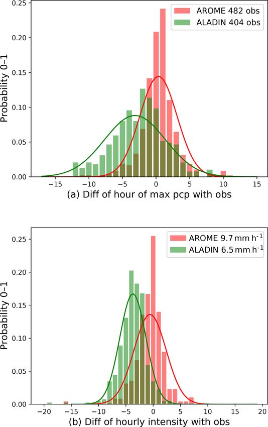
1318 D. Belušić et al.: HCLIM38
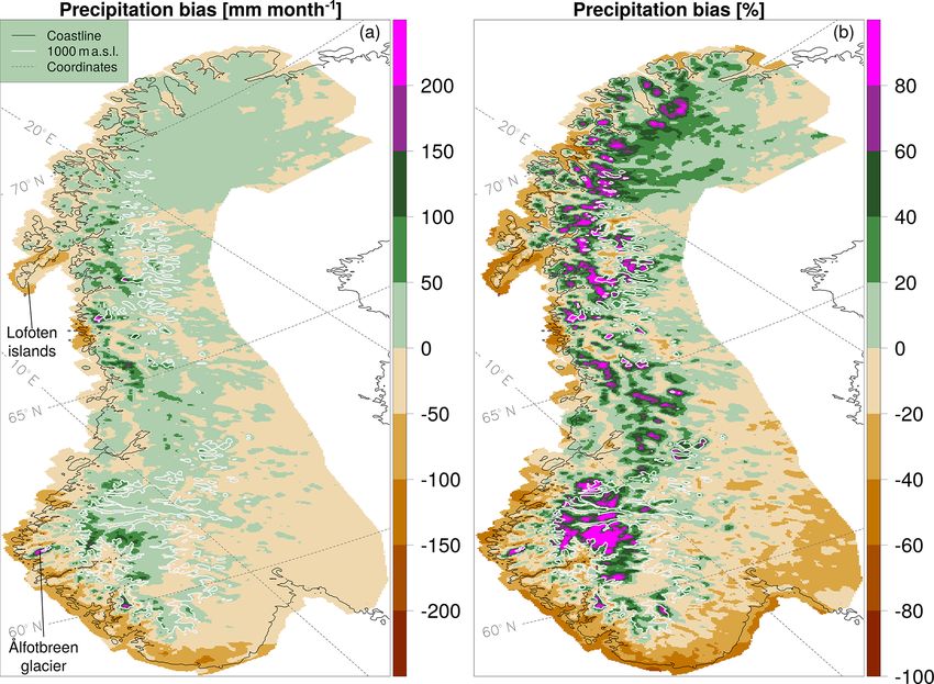
Figure 3. (a) Absolute and (b) relative precipitation differences between HCLIM38-AROME and seNorge for the time period 2004–2015.
ences are mostly seen in connection with mountainous re- 3.1.2 Norway
gions. This is also the case for temperature in winter. For
example, the negative temperature bias in winter over Scan- Due to its complex topography and the exposure of the west-
dinavia is mostly associated with 2–4 ◦ C lower values over ern coast to large amounts of moisture transported over the
the Scandinavian mountains. At lower altitudes the tempera- North Atlantic, Norway is a challenging area for which to
ture is much better represented by the model (Fig. S1). Still, provide accurate climate model simulations and constitutes
the cold bias in HCLIM38-ALADIN is present throughout an ideal testing environment. To evaluate the performance of
most seasons and is spatially widespread over Europe. The the HCLIM38-AROME model in this region at convection-
reason for this systematic bias is not yet known and needs to permitting scales, it was run at 2.5 km for an area covering
be further investigated. Finally, we note that for the two ver- Norway, parts of Finland, Sweden and Russia for the time pe-
sions of ALADIN, HCLIM38-ALADIN consistently shows riod 2004–2016 (Crespi et al., 2019), downscaling the ERA-
lower temperatures than CNRM-ALADIN53 for large parts Interim reanalysis. An intermediate HCLIM38-ALARO sim-
of Europe, apart from western and southern Europe. The pre- ulation at 24 km resolution was used to avoid an excessively
cipitation differences compared to E-OBS, however, are gen- large jump across the boundaries (results not analysed here).
erally smaller in HCLIM38-ALADIN. We conclude that the For the evaluation over Norway, we use the gridded obser-
performance of HCLIM38-ALADIN over Europe, in terms vation dataset seNorge v2.1 for precipitation (Lussana et al.,
of multi-year means of T2m and precipitation, is generally 2018a) and temperature (Lussana et al., 2018b); seNorge pro-
within the range of the performance of other RCMs used vides daily precipitation and temperature back to 1957 at a
within EURO-CORDEX. grid resolution of 1 km. The dataset has a special focus on
providing meteorological input for snow and hydrological
simulations at the regional or national level. Thus, it not only
covers the Norwegian mainland but also neighbouring areas
in Finland, Sweden and Russia to include regions impacting
Geosci. Model Dev., 13, 1311–1333, 2020 www.geosci-model-dev.net/13/1311/2020/
D. Belušić et al.: HCLIM38                                                                                                  1319

                                                                     Generally, HCLIM38-AROME shows an underestimation
                                                                  of precipitation at the south-western coast and over the Lo-
                                                                  foten islands, while precipitation in the mountains is over-
                                                                  estimated (Fig. 3). The largest differences appear in autumn
                                                                  and winter (not shown). Values for precipitation that are too
                                                                  high can also be seen for spring and summer over central–
                                                                  southern Norway. Similar differences have been shown by
                                                                  Müller et al. (2017) for the Nordic operational NWP setup
                                                                  of HARMONIE–AROME and by Crespi et al. (2019) com-
                                                                  paring the HCLIM38-AROME precipitation data to observed
                                                                  precipitation.
                                                                     However, despite the biases found in simulated precipi-
                                                                  tation, the HCLIM38-AROME data have been successfully
                                                                  used by Crespi et al. (2019) together with in situ observa-
                                                                  tions to obtain improved monthly precipitation climatologies
                                                                  over Norway. The high-resolution model data are used to pro-
                                                                  vide a spatial reference field for an improved interpolation of
                                                                  the in situ observations where there are no measurements.
                                                                  The result is not a purely bias-corrected RCM dataset, nor
                                                                  are the in situ observations corrected. The approach is used
                                                                  to overcome the uneven station network over Norway, and it
                                                                  was shown that the simulated precipitation could be used to
                                                                  improve the climatologies significantly, especially over the
                                                                  most remote regions. For instance, for the wettest area in
                                                                  Norway around Ålfotbreen, the combined data result in a
                                                                  mean annual precipitation of over 5700 mm. Measurements
                                                                  of snow accumulation during the winter half-year together
                                                                  with estimates of drainage from river basins (performed by
                                                                  the Norwegian Water Resources and Energy Directorate) in-
                                                                  dicate mean annual precipitation amounts over 5500 mm in
                                                                  the area (Teigen, 2005). The purely observation-based esti-
Figure 4. Annual temperature differences between HCLIM38-         mates are almost 2000 mm lower.
AROME and seNorge for the time period 2004–2015.
                                                                     The combined dataset shows systematically higher precip-
                                                                  itation values than seNorge for the observation-sparse moun-
                                                                  tainous regions. As the seNorge dataset is likely to underes-
the Norwegian water balance. The station data are retrieved       timate precipitation in these areas (Lussana et al., 2018a) we
from MET Norway’s climate database and the European Cli-          expect this to be an improvement. However, whether this is
mate Assessment and Dataset (ECA&D, Klein Tank et al.,            true still needs to be verified e.g. by the use of hydrological
2002). More details on the spatial interpolation schemes and      simulations (Lussana et al., 2019).
the dataset in general are given in Lussana et al. (2018a, b).       Annual mean temperature in HCLIM38-AROME is gen-
   Note that gridded observation datasets in remote regions       erally lower than in seNorge, but the differences are small
of Norway should be considered with caution. For certain re-      (Fig. 4). Averaged over the whole area, HCLIM38-AROME
gions of Norway it may be difficult to judge the quality of       is about 1 ◦ C colder than seNorge. The differences range
the seNorge data due to the inhomogeneous station distribu-       from about −7 to 4 ◦ C, but for most of the area, the tem-
tion. While terrain height can reach 2000 m or more, most         perature differences are below ±2 ◦ C and larger biases are
stations are located below 1000 m. There is also a differ-        restricted to the mountains. All seasons show similar patterns
ence in the station density between the southern and northern     to the annual biases with the largest differences in the moun-
parts, with a higher density in the south of Norway (Lussana      tains, but the general increase in the bias with altitude is most
et al., 2019). For precipitation, Lussana et al. (2018a) have     pronounced in winter (not shown).
shown that seNorge2 gives values that are too low in very
data-sparse areas. For temperature, an evaluation in Lussana      3.1.3   Summer precipitation over the Netherlands and
et al. (2018b) has shown that the interpolation actually yields           Germany
unbiased estimates, with the exception of a warm bias for
very low temperatures, and that the grid point estimates show     Better resolving summertime precipitation is arguably the
a precision of 0.8 to 2.4 ◦ C.                                    most important reason for running CPRCMs and a pri-

www.geosci-model-dev.net/13/1311/2020/                                              Geosci. Model Dev., 13, 1311–1333, 2020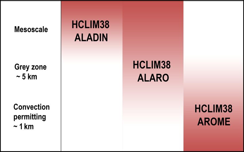
1320                                                                                                      D. Belušić et al.: HCLIM38

Figure 5. (a) Diurnal cycle of two high percentiles (90th and 99th percentile) and the average of the FLDMAX hourly precipitation distri-
bution (April–September) for radar, CPRCM and driving RCM. Probability of exceedance (April–September) for (b) the FLDMAX precipi-
tation and (c) the FLDMEAN precipitation (note the difference in the vertical scale). Confidence levels (95 %) obtained using bootstrapping
are indicated by shading.

mary variable for which we anticipate added value com-                     For the evaluation of the CPRCMs to rain radar over
pared to coarser-resolution RCM models. In this section we              the Netherlands, we can only use output from E1 since the
discuss statistics of summer precipitation in two 10-year               E2 domain does not cover the Netherlands. The radar data
ERA-Interim forced climate simulations for the period 2000–             are an hourly gridded product (2.4 km horizontal resolu-
2009, carried out with HCLIM38-AROME at convection-                     tion) that has been calibrated against automatic and man-
permitting scales. The focus will be on the summer half-year            ual rain gauges (Overeem et al., 2009). Data from both
(April–September). The first CPRCM experiment (E1) con-                 the CPRCM (HCLIM38-AROME, 2.5 km) and the RCM
ducted by KNMI receives lateral boundary conditions from                (RACMO2, 0.11◦ ) are put on the radar grid using nearest-
the RCM RACMO2 (van Meijgaard et al., 2012). In the sec-                neighbour interpolation. Two statistics are studied. First, we
ond experiment (E2) conducted by SMHI, the host model is                look at hourly spatial precipitation maxima found within the
HCLIM38-ALADIN. Both host models are forced by ERA-                     Netherlands. We call this the hourly FLDMAX statistic. The
Interim. For both E1 and E2 the domain covers the pan-                  analysis focuses on model performance at the grid scale, and
Alpine region as defined in the CORDEX FPS on convection                here we expect to find added value. Note that in this for-
(Coppola et al., 2018), but the E1 domain extends substan-              mulation the FLDMAX does not account for the spatial ex-
tially further to the north-west, covering a large part of the          tent of the precipitation, nor does it account for the possi-
North Sea. Output is compared to two types of observations:             ble existence of several convective clusters at the same hour.
radar data (for the Netherlands) and rain gauges (for a part of         Secondly, we study the hourly FLDMEAN statistic (i.e. the
Germany).                                                               hourly area-average precipitation). If a CPRCM outperforms
                                                                        its host model for the latter statistic, this is an example of

Geosci. Model Dev., 13, 1311–1333, 2020                                                    www.geosci-model-dev.net/13/1311/2020/
D. Belušić et al.: HCLIM38 1321 Figure 6. As in Fig. 5, but for the evaluation over low-lying (< 500 m) German rain gauges. (a) Diurnal cycle of the 90th and 99th percentile of the FLDMAX precipitation. (b) Probability of exceedance (Apr–Sep) for the FLDMAX precipitation. Confidence levels (95 %) obtained using bootstrapping are indicated by shading. E1 and E2 denote two experiments with different modelling setups (see text for details). upscale added value: the higher horizontal resolution also the Netherlands), HCLIM38-AROME generally outperforms pays off at larger spatial scale. This is not guaranteed, es- RACMO2, especially for the larger precipitation amounts. pecially not in winter, when precipitation is often caused by It could be argued that a non-CPRCM cannot be expected large-scale weather systems. Confidence intervals (95 %) are to reproduce the radar-observed precipitation statistics be- estimated using bootstrapping. The bootstrapping technique cause of its coarser resolution. For this reason, we have re- consists of constructing a large number of “synthetic” time computed the statistics shown in Fig. 5 using the data that series by resampling days from the original time series (sam- were re-gridded to the 12 km RCM grid prior to computa- pling with replacement) and computing the target statistic for tion. This upscaling to 12 km was done using simple con- each of the resamples. This gives an empirical distribution for servative interpolation. Figure S3 shows that the differences the target statistic, from which the confidence interval can be between CPRCMs and RCMs remain qualitatively the same estimated. The resulting estimate is overconfident as it ig- after upscaling to the RCM grid. Therefore, even at these spa- nores time correlations. tial scales there is clear added value of the CPRCM. We expect the largest benefits of using a high-resolution For the evaluation of the CPRCMs over Germany, we com- model at the finest scales, which cannot be reached by pare E1 and E2 to hourly rain gauge data. As a proxy for the the non-CPRCM. This is confirmed for the Netherlands in rain gauge location we use the nearest model grid point. In Fig. 5a, which shows for each hour an estimate of the average addition, we consider only stations that have an altitude lower and the 90th and 99th percentile of the FLDMAX precipita- than 500 m (see Fig. S4 for the rain gauges involved). Simi- tion; 3-hourly sliding windows are used to improve statisti- larly to the evaluation done over the Netherlands, we use the cal robustness, and confidence bands were determined using FLDMAX and FLDMEAN approach in which the appropri- bootstrap resampling on hourly basis. HCLIM38-AROME ate statistical operator is applied over the hourly data. simulates the diurnal cycle very well. Although the diurnal The differences between CPRCMs and RCMs for FLD- cycle of HCLIM38-AROME is about an hour delayed with MAX for Germany are similar to the results for the Nether- respect to the radar observations, it is much improved com- lands presented above, with the CPRCM agreeing better pared to RACMO2, which hardly shows signs of a diurnal with observations (Fig. 6). Note how similar the HCLIM38- cycle. Results for the winter half-year are qualitatively sim- AROME simulations are, despite the rather different charac- ilar, but the amplitude of the daily cycle is much less pro- teristics of their host model. Although the diurnal cycle is nounced (not shown). For the FLDMEAN statistic, the am- better represented by the CPRCMs, the modelled late after- plitude in the diurnal cycle is dampened, and RACMO2 and noon peaks are too high. It appears that the overestimation HCLIM38-AROME are generally more similar (not shown). of the peak is related to the elevation: if we constrain to the Figure 5b and c show the precipitation distributions as ex- subset spanned by gauges at lower elevation, the CPRCMs ceedance plots. The exceedance plots are computed by sim- agree better with the observations (not shown). The overesti- ple ordering of the FLDMAX or FLDMEAN data and in- mation of intense precipitation (10–40 mm h−1 ) is consistent ferring the empirical probability of a given value based on with the analysis of the UKMO and ETH-COSMO models its order position. Not only at the grid scale (FLDMAX), in Berthou et al. (2018) for Germany. Similar to the results but also at the largest spatial scale available (FLDMEAN, www.geosci-model-dev.net/13/1311/2020/ Geosci. Model Dev., 13, 1311–1333, 2020
1322                                                                                               D. Belušić et al.: HCLIM38

over the Netherlands, the differences between CPRCMs and         from each other, will be verified below and has been shown
RCMs are smaller for the FLDMEAN statistic (not shown).          in other studies (e.g. Brown et al., 2010).
                                                                     Two aspects of summer (JJA) precipitation are studied:
3.1.4   Summer precipitation over the Iberian Peninsula          the timing of the maximum hourly precipitation within a
                                                                 day and the hourly intensity. At hourly scales we expect the
The Mediterranean region is characterized by a complex           convection-permitting nonhydrostatic physics (AROME) to
morphology due to the presence of many sharp orographic          better reproduce the precipitation characteristics compared
features: high mountain ridges surround the Mediterranean        to the hydrostatic physics (ALADIN). For the timing and in-
Sea on almost every side, the presence of distinct basins        tensity we calculate for each rain gauge the 10-year mean
and gulfs, and islands and peninsulas of various sizes. These    of the hour of maximum precipitation in a day and the cor-
characteristics have important consequences on both sea and      responding hourly intensity, respectively. The same is cal-
atmospheric circulations because they introduce large spa-       culated for the two models after interpolating the modelled
tial variability and the presence of many subregional and        precipitation to the nearest-neighbour observation. The 10-
mesoscale features (e.g. Lionello et al., 2006). Moreover,       year observation mean is subtracted from the 10-year model
the Mediterranean region is considered to be a hotspot for       means to get the difference in every point. These differences
climate change (e.g. Giorgi, 2006). It is frequently exposed     for every location are pooled together, and PDFs of the tim-
to recurring droughts and torrential rainfall events, both of    ing differences and hourly intensity differences are obtained
which are projected to become more frequent and/or intense       for AROME and ALADIN. Gaussian distributions are fitted
as a result of future climate change. Therefore, it is an area   to the PDFs with the same mean and variance for a clearer
where climate models have to be tested. In this study we         comparison.
focus on eastern Spain in summer (JJA) when precipita-               Several hourly thresholds have been tested (0, 5, 10, 15
tion events are scarce and mainly convective (e.g. Alham-        and 20 mm h−1 ), filtering out hourly precipitation below each
moud et al., 2014). Our aim is to study the performance          threshold. Finally, we use the threshold of 5 mm h−1 to re-
of HCLIM38 in representing convective precipitation in dry       move periods with weak precipitation while keeping a suffi-
zones at high temporal and spatial resolution.                   cient number of events for robust statistics. The number of
   We compare results from two HCLIM38 simulations, one          points fulfilling this condition is near 500 for AROME and
at high resolution with the AROME configuration and an-          around 400 for ALADIN.
other at lower resolution with the ALADIN configuration,             The histograms of the differences of the hour of max-
against hourly precipitation records. These are the experi-      imum precipitation and intensity between models and ob-
ments performed.                                                 servations are shown in Fig. 7. The distributions of differ-
                                                                 ences for both timing and intensity are centred at zero for
  – AROME: 10 years (1990–1999), 2.5 km resolution,
                                                                 HCLIM38-AROME, while they are shifted to negative val-
    Iberian Peninsula
                                                                 ues for HCLIM38-ALADIN. This indicates that the AL-
  – ALADIN: 10 years (2005–2014), 12 km resolution, Eu-          ADIN physics underestimate both the timing and inten-
    rope                                                         sity of maximum hourly precipitation, while the convection-
                                                                 permitting physics AROME are able to reproduce both re-
   Both simulations were forced directly with ERA-Interim        alistically. In the case of timing the PDF of HCLIM38-
data at the boundaries. The simulations are compared with        AROME is narrower, while HCLIM38-ALADIN shows a
a dense set of around 500 automatic and manual rain              wider spread in the hour of maximum precipitation. For the
gauges recording hourly precipitation that are distributed       intensity both models have similar spread.
over eastern Spain (Fig. S5). These observations are ex-             Even though HCLIM38-ALADIN has 7 years of over-
tracted from the National Weather Data Bank of AEMET             lap with observations and HCLIM38-AROME has none,
(Santos-Burguete, 2018, Chapter 9) and have been used in         HCLIM38-AROME is closer to the observations. Therefore,
other studies of intense precipitation events (e.g. Khodayar     it seems that the decadal variability in the distribution is suffi-
et al., 2016; Riesco-Martín et al., 2014).                       ciently small to allow for a comparison between observations
   The selected period for observations is 2008–2018 be-         and simulations of different (but close) periods in this case.
cause hourly data from automatic stations started to be avail-       In conclusion, the convection-permitting model
able in 2008. This period has 7 years of overlap with the        HCLIM38-AROME shows a clear improvement in the
HCLIM38-ALADIN simulation, but it does not overlap the           representation of key characteristics of precipitation as
HCLIM38-AROME simulation. We assume that the precip-             exemplified by timing and hourly intensity compared
itation characteristics have not substantially changed in the    to the hydrostatic model HCLIM38-ALADIN. While
last 30 years and that in two nearby 10-year periods the mean    HCLIM38-ALADIN underestimates the mean values of
statistics calculated from hourly precipitation are compara-     both variables, HCLIM38-AROME shows very small biases
ble. The assumption that rainfall characteristics are not de-    for the threshold used (> 5 mm h−1 ). In accordance with
pendent on the period analysed, when periods are not far         previous CPRCM studies (e.g. Ban et al., 2014; Berthou

Geosci. Model Dev., 13, 1311–1333, 2020                                             www.geosci-model-dev.net/13/1311/2020/
D. Belušić et al.: HCLIM38 1323
on Greenland (e.g. Ettema et al., 2010; Lucas-Picher et al.,
2012; Rae et al., 2012; Noël et al., 2018).
HCLIM38 can run in a polar stereographic projection,
which is ideal for the Arctic region. Here, we present the re-
sults from three HCLIM38 simulations, all forced by ERA-
Interim during the summer of 2014 over a domain covering
the Arctic region and reaching 60◦ N across all longitudes.
The simulations all use the default HCLIM38 setup and do
not employ any type of nudging despite the large domain.
The three experiments are the following.
– ALARO24: HCLIM38-ALARO, 24 km resolution
– ALADIN24: HCLIM38-ALADIN, 24 km resolution
– ALADIN12: HCLIM38-ALADIN, 12 km resolution
This ensemble allows for the assessment of (1) the
performance of HCLIM38 compared to observed condi-
tions, (2) the differences between identical simulations with
ALARO and ALADIN physics, and (3) the impact of in-
creased resolution (in ALADIN only).
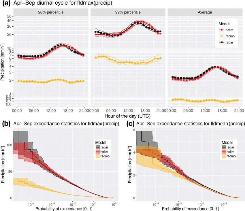
The model performance is assessed over Greenland using
in situ observations at 16 locations from the Programme for
Monitoring of the Greenland Ice Sheet (PROMICE; van As
et al., 2011; Fausto and van As, 2019), a network of auto-
matic weather stations placed on the Greenland Ice Sheet.
We assess the monthly and seasonal mean temperature in
the model grid cells closest to the stations, which are mainly
located in the ablation zone, i.e. the lower-elevation part of
Figure 7. Histograms of differences between models (HCLIM- the ice sheet, which experiences melt during summer. To en-
AROME 2.5 km and HCLIM-ALADIN 12 km) and observations of sure a consistent bias assessment, the simulated temperatures
the 10-year mean of (a) the hour of maximum precipitation and have been corrected for the elevation difference between the
(b) the corresponding maximum hourly intensity for the hourly in- station location and the model grid cell. Figure 8a shows
tensity threshold of 5 mm h−1 . The legend shows (a) the number of seasonal (JJA) mean temperature in the model and the bias
stations used in the comparison for each of the models and (b) the at the individual PROMICE stations, where the simulated
mean intensity for each model. The mean intensity in observations temperature is adjusted using a lapse rate of 6.0 ◦ C km−1
is 10.2 mm h−1 . (based on observed summer conditions; Erokhina et al.,
2017). Further, we have calculated the number of days on
which these locations experience melt, here defined as near-
et al., 2018), the main reason for this improvement is that surface air temperature above 0 ◦ C. This is evaluated using
AROME explicitly resolves deep convection (Seity et al., the Tmax, i.e. the daily maximum temperature experienced
2011; Bengtsson et al., 2017), while HCLIM38-ALADIN in a given grid cell on the time step scale (time steps are
parameterizes it. 10 min for ALARO24 and ALADIN24 and 5 min for AL-
ADIN12). Here the simulated temperature is not lapse-rate-
3.2 First simulations over the Arctic region corrected; melt is chosen as an additional metric in order to
assess the model representation of the cryospheric feedback
The Arctic region is an excellent test bed for climate models. processes that are central to the Arctic climate.
Interactions between the atmosphere, ocean and cryosphere Compared to the driving ERA-Interim reanalysis data,
are central in shaping the regional climate, and biases in the all the HCLIM38 runs provide more detailed spatial pat-
simulated climate will be greatly affected by the model’s terns over complex terrain, such as in mountainous regions
ability to capture the correct build-up and melt of snow and and on the slopes of the ice sheet. The comparison to the
ice. Previous studies have indicated the challenges in simu- PROMICE observations reveals that all three configurations
lating the Arctic climate and highlighted the fact that more of HCLIM38 are generally colder and have lower average
detailed surface schemes and very high resolution may be bias compared to the coarser ERA-Interim (approximately
needed to improve model performance in the Arctic and 80 km resolution). The PROMICE stations are all located on
www.geosci-model-dev.net/13/1311/2020/ Geosci. Model Dev., 13, 1311–1333, 2020You can also read