Present and future aerosol impacts on Arctic climate change in the GISS-E2.1 Earth system model - Recent
←
→
Page content transcription
If your browser does not render page correctly, please read the page content below
Atmos. Chem. Phys., 21, 10413–10438, 2021
https://doi.org/10.5194/acp-21-10413-2021
© Author(s) 2021. This work is distributed under
the Creative Commons Attribution 4.0 License.

Present and future aerosol impacts on Arctic climate change in the
GISS-E2.1 Earth system model
Ulas Im1,2 , Kostas Tsigaridis3,4 , Gregory Faluvegi3,4 , Peter L. Langen1,2 , Joshua P. French5 , Rashed Mahmood6 ,
Manu A. Thomas7 , Knut von Salzen8 , Daniel C. Thomas1,2 , Cynthia H. Whaley8 , Zbigniew Klimont9 , Henrik Skov1,2 ,
and Jørgen Brandt1,2
1 Department   of Environmental Science, Aarhus University, Roskilde, Denmark
2 Interdisciplinary Centre for Climate Change, Aarhus University, Roskilde, Denmark
3 Center for Climate Systems Research, Columbia University, New York, NY, USA
4 NASA Goddard Institute for Space Studies, New York, NY, USA
5 Department of Mathematical and Statistical Sciences, University of Colorado Denver, Denver, USA
6 Barcelona Supercomputing Center, Barcelona, Spain
7 Swedish Meteorological and Hydrological Institute, Norrköping, Sweden
8 Canadian Centre for Climate Modelling and Analysis, Environment and Climate Change Canada,

Victoria, British Columbia, Canada
9 International Institute for Applied Systems Analysis (IIASA), Laxenburg, Austria

Correspondence: Ulas Im (ulas@envs.au.dk)

Received: 20 December 2020 – Discussion started: 7 January 2021
Revised: 2 June 2021 – Accepted: 10 June 2021 – Published: 9 July 2021

Abstract. The Arctic is warming 2 to 3 times faster than         smaller biases in aerosol levels compared to atmosphere-only
the global average, partly due to changes in short-lived cli-    simulations without nudging.
mate forcers (SLCFs) including aerosols. In order to study          Arctic BC, organic aerosol (OA), and SO2−   4 burdens de-
the effects of atmospheric aerosols in this warming, recent      crease significantly in all simulations by 10 %–60 % fol-
past (1990–2014) and future (2015–2050) simulations have         lowing the reductions of 7 %–78 % in emission projec-
been carried out using the GISS-E2.1 Earth system model to       tions, with the Eclipse ensemble showing larger reductions
study the aerosol burdens and their radiative and climate im-    in Arctic aerosol burdens compared to the CMIP6 ensem-
pacts over the Arctic (> 60◦ N), using anthropogenic emis-       ble. For the 2030–2050 period, the Eclipse ensemble simu-
sions from the Eclipse V6b and the Coupled Model Inter-          lated a radiative forcing due to aerosol–radiation interactions
comparison Project Phase 6 (CMIP6) databases, while global       (RFARI ) of −0.39 ± 0.01 W m−2 , which is −0.08 W m−2
annual mean greenhouse gas concentrations were prescribed        larger than the 1990–2010 mean forcing (−0.32 W m−2 ),
and kept fixed in all simulations.                               of which −0.24 ± 0.01 W m−2 was attributed to the anthro-
   Results showed that the simulations have underestimated       pogenic aerosols. The CMIP6 ensemble simulated a RFARI
observed surface aerosol levels, in particular black carbon      of −0.35 to −0.40 W m−2 for the same period, which is
(BC) and sulfate (SO2− 4 ), by more than 50 %, with the small-   −0.01 to −0.06 W m−2 larger than the 1990–2010 mean
est biases calculated for the atmosphere-only simulations,       forcing of −0.35 W m−2 . The scenarios with little to no miti-
where winds are nudged to reanalysis data. CMIP6 simula-         gation (worst-case scenarios) led to very small changes in the
tions performed slightly better in reproducing the observed      RFARI , while scenarios with medium to large emission mit-
surface aerosol concentrations and climate parameters, com-      igations led to increases in the negative RFARI , mainly due
pared to the Eclipse simulations. In addition, simulations       to the decrease in the positive BC forcing and the decrease
where atmosphere and ocean are fully coupled had slightly        in the negative SO2− 4 forcing. The anthropogenic aerosols
                                                                 accounted for −0.24 to −0.26 W m−2 of the net RFARI in

Published by Copernicus Publications on behalf of the European Geosciences Union.
10414                                             U. Im et al.: Present and future aerosol impacts on Arctic climate change

2030–2050 period, in Eclipse and CMIP6 ensembles, respec-         ide (SO2 ), absorbs negligible solar radiation and cools the
tively. Finally, all simulations showed an increase in the Arc-   climate by scattering solar radiation back to space. Organic
tic surface air temperatures throughout the simulation period.    carbon (OC), which is co-emitted with BC during combus-
By 2050, surface air temperatures are projected to increase       tion, both scatters and absorbs solar radiation and therefore
by 2.4 to 2.6 ◦ C in the Eclipse ensemble and 1.9 to 2.6 ◦ C in   causes cooling in some environments and warming in others.
the CMIP6 ensemble, compared to the 1990–2010 mean.               Highly reflective regions such as the Arctic are more likely
   Overall, results show that even the scenarios with largest     to experience warming effects from these organic aerosols
emission reductions leads to similar impact on the future         (e.g., Myhre et al., 2013).
Arctic surface air temperatures and sea-ice extent compared          Aerosols also influence climate via indirect mechanisms.
to scenarios with smaller emission reductions, implying re-       After being deposited on snow and ice surfaces, BC can
ductions of greenhouse emissions are still necessary to miti-     amplify ice melt by lowering the albedo and increasing so-
gate climate change.                                              lar heating of the surface (AMAP, 2015). Aerosols also af-
                                                                  fect cloud properties, including their droplet size, lifetime,
                                                                  and vertical extent, thereby influencing both the shortwave
                                                                  cooling and longwave warming effects of clouds. Globally,
1   Introduction                                                  this indirect cloud forcing from aerosols is likely larger than
                                                                  their direct forcing, although the indirect effects are more
The Arctic is warming 2 to 3 times faster than the global av-     uncertain and difficult to accurately quantify (IPCC, 2013).
erage (IPCC, 2013; Lenssen et al., 2019). This is partly due      Moreover, Arctic cloud impacts are distinct from global im-
to internal Arctic feedback mechanisms, such as the snow          pacts, owing to the extreme seasonality of solar radiation in
and sea-ice–albedo feedback, where melting ice leads to in-       the Arctic, unique characteristics of Arctic clouds (e.g., high
creased absorption of solar radiation, which further enhances     frequency of mixed-phase occurrence), and rapidly evolving
warming in the Arctic (Serreze and Francis, 2006). How-           sea-ice distributions. Together, they lead to complicated and
ever, Arctic temperatures are also affected by interactions       unique phenomena that govern Arctic aerosol abundances
with warming at lower latitudes (e.g., Stuecker et al., 2018;     and climate impacts (e.g., Willis et al., 2018; Abbatt et al.,
Graversen and Langen, 2019; Semmler et al., 2020) and by          2019). The changes taking place in the Arctic have conse-
local in situ response to radiative forcing due to changes in     quences for how SLCFs affect the region. For example, re-
greenhouse gases and aerosols in the area (Shindell, 2007;        ductions in sea-ice extent, thawing of permafrost, and humid-
Stuecker et al., 2018). In addition to warming induced by in-     ification of the Arctic troposphere can affect the emissions,
creases in global atmospheric carbon dioxide (CO2 ) concen-       lifetime, and radiative forcing of SLCFs within the Arctic (J.
trations, changes in short-lived climate forcers (SLCFs) such     L. Thomas et al., 2019).
as tropospheric ozone (O3 ), methane (CH4 ), and aerosols            The effect of aerosols on the Arctic climate through the
(e.g., black carbon (BC) and sulfate (SO2−4 )) in the Northern    effects of scattering and absorption of radiation, clouds,
Hemisphere (NH) have contributed substantially to the Arc-        and surface ice/snow albedo has been investigated in pre-
tic warming since 1890 (Shindell and Faluvegi, 2009; Ren          vious studies (i.e., Clarke and Noone, 1985; Flanner et al.,
et al., 2020). This contribution from SLCFs to Arctic heat-       2007; Shindell et al., 2012; Bond et al., 2013; Dumont et
ing together with efficient local amplification mechanisms        al., 2014). The impact of aerosols on the Arctic climate
puts a high priority on understanding the sources and sinks       change is mainly driven by a response to remote forcings
of SLCFs at high latitudes and their corresponding climatic       (Gagné et al., 2015; Sand et al., 2015; Westervelt et al.,
effects.                                                          2015). Long-range transport is known to play an important
   SLCFs include all atmospheric species, which have short        role in the Arctic air pollution levels, and much of the at-
residence times in the atmosphere relative to long-lived          tention on aerosol climatic effects in the Arctic was focused
greenhouse gases and have the potential to affect Earth’s ra-     on long-range-transported anthropogenic pollution (Arctic
diative energy budget. Aerosols are important SLCFs and           haze) in the past (Quinn et al., 2007; AMAP, 2015; Ab-
are a predominant component of air quality that affects hu-       batt et al., 2019). Long-range transport of BC and SO2−     4 ,
man health (Burnett et al., 2018; Lelieveld et al., 2019). They   in particular from Asia, traveling at a relatively high al-
mostly affect climate by altering the amount of solar energy      titude to the Arctic can be deposited on the snow and
absorbed by Earth, as well as changing the cloud properties       ice, contributing to surface albedo reduction. On the other
and indirectly affecting the scattering of radiation, and are     hand, there has been increasing attention on the local Arc-
efficiently removed from the troposphere within several days      tic aerosol sources, in particular natural aerosol sources
to weeks. BC, which is a product of incomplete combustion         (Schmale et al., 2021). Lewinschal et al. (2019) estimated
and open biomass/biofuel burning (Bond et al., 2014, 2013),       an Arctic surface temperature change per unit global sul-
absorbs a high proportion of incident solar radiation and         fur emission of −0.020 to −0.025 K Tg−1 S yr−1 . Sand et
therefore warms the climate system (Jacobson, 2001). SO2−   4 ,   al. (2020) calculated an Arctic surface air temperature re-
which is formed primarily through oxidation of sulfur diox-       sponse of 0.06–0.1 K Tg−1 BC yr−1 to BC emissions in Eu-

Atmos. Chem. Phys., 21, 10413–10438, 2021                                         https://doi.org/10.5194/acp-21-10413-2021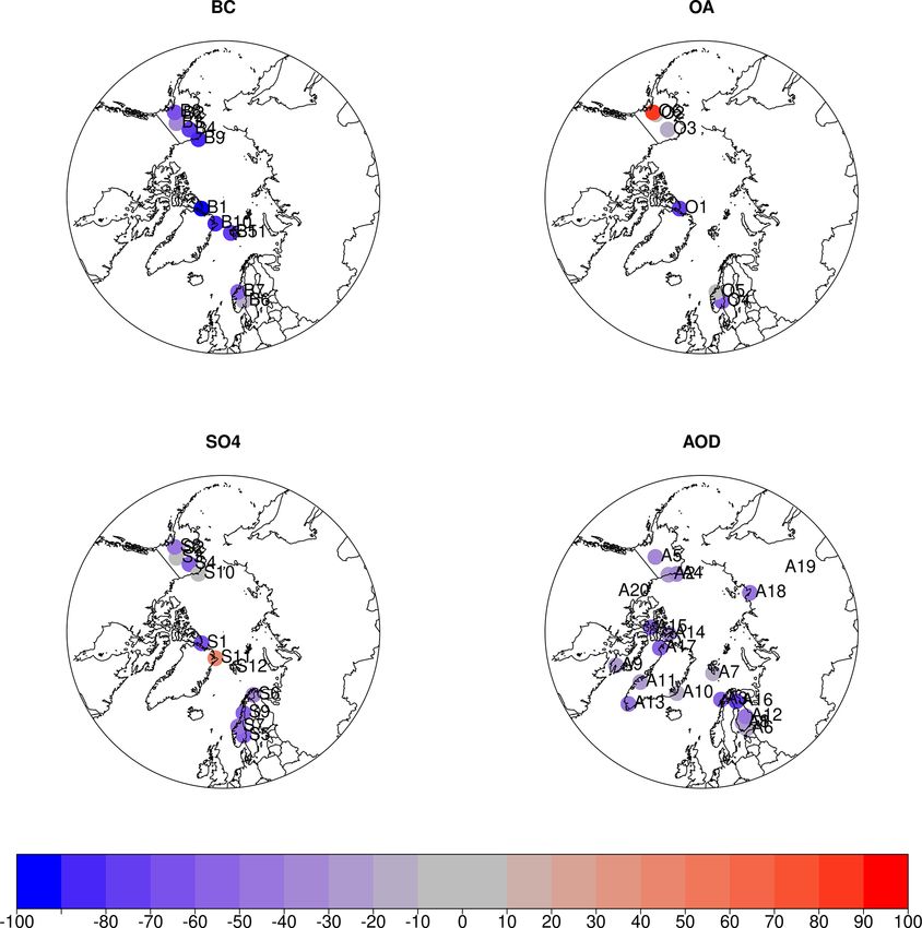
U. Im et al.: Present and future aerosol impacts on Arctic climate change                                                 10415

rope and North America and a slightly lower response of           uation of the model and the climate impact. Section 2 in-
0.05–0.08 K Tg−1 BC yr−1 to Asian emissions. Breider et al.       troduces the GISS-E2.1 model, the anthropogenic emissions,
(2017) reported a shortwave (SW) aerosol radiative forc-          and the observation datasets used in model evaluation. Sec-
ing (ARF) of −0.19 ± 0.05 W m−2 at the top of the atmo-           tion 3 presents results from the model evaluation as well as
sphere (TOA) over the Arctic, which reflects the balance be-      recent past and future trends in simulated aerosol burdens, ra-
tween sulfate cooling (−0.60 W m−2 ) and black carbon (BC)        diative forcing, and climate change over the Arctic. Section 4
warming (+0.44 W m−2 ). Schacht et al. (2019) calculated          summarizes the overall findings and the conclusions.
a direct radiative forcing of up to 0.4 W m−2 over the Arc-
tic using the ECHAM6.3-HAM2.3 global aerosol–climate
model. Markowicz et al. (2021), using the Navy Aerosol            2     Materials and methods
Analysis and Prediction System (NAAPS) radiative trans-
fer model, calculated a total aerosol forcing over the Arc-       2.1    Model description
tic (> 70.5◦ N) of −0.4 W m−2 . Ren et al. (2020) simulated
0.11 and 0.25 W m−2 direct and indirect warming in 2014–          GISS-E2.1 is the CMIP6 version of the GISS modelE Earth
2018 compared to 1980–1984 due to reductions in sulfate,          system model, which has been validated extensively over the
using the CAM5-EAST global aerosol–climate model. They            globe (Kelley et al., 2020; Bauer et al., 2020) as well as
also reported that the aerosols produced an Arctic surface        regionally for air pollutants (Turnock et al., 2020). A full
warming of +0.30 ◦ C during 1980–2018, explaining about           description of GISS-E2.1 and evaluation of its coupled cli-
20 % of the observed Arctic warming observed during the           matology during the satellite era (1979–2014) and the re-
last four decades, while according to Shindell and Faluvegi       cent past ensemble simulation of the atmosphere and ocean
(2009), aerosols contributed 1.09 ± 0.81 ◦ C to the observed      component models (1850–2014) are described in Kelly et al.
Arctic surface air temperature increase of 1.48 ± 0.28 ◦ C ob-    (2020) and Miller et al. (2020), respectively. GISS-E2.1 has
served in 1976–2007. AMAP (2015), based on four Earth             a horizontal resolution of 2◦ in latitude by 2.5◦ in longitude
system models (ESMs), estimated a total Arctic surface air        and 40 vertical layers extending from the surface to 0.1 hPa
temperature response due to the direct effect of current global   in the lower mesosphere. The tropospheric chemistry scheme
combustion-derived BC, OC, and sulfur emissions to be             used in GISS-E2.1 (Shindell et al., 2013) includes inorganic
+0.35 ◦ C, of which +0.40 ◦ C was attributed to BC in the         chemistry of Ox , NOx , HOx , and CO and organic chemistry
atmosphere, +0.22 ◦ C to BC in snow, −0.04 ◦ C to OC, and         of CH4 and higher hydrocarbons using the CBM4 scheme
−0.23 ◦ C to SO2− 4 . On the other hand, Stjern et al. (2017)     (Gery et al., 1989) and the stratospheric chemistry scheme
and Takemura and Suzuki (2019) showed that due to the             (Shindell et al., 2013), which includes chlorine and bromine
rapid adjustments from BC, mitigation of BC emissions can         chemistry together with polar stratospheric clouds.
lead to weak responses in the surface temperatures. Samset           In the present work, we used the one-moment aerosol
et al. (2018), using a multi-model ensemble of ocean coupled      scheme (OMA: Bauer et al., 2020, and references therein),
ESMs, where aerosol emissions were either kept at present-        which is a mass-based scheme in which aerosols are as-
day conditions or anthropogenic emissions of SO2 and fossil       sumed to remain externally mixed. All aerosols have a pre-
fuel BC and OC were set to zero, showed that Arctic sur-          scribed and constant size distribution, with the exception of
face warming due to aerosol reductions can reach up to 4 ◦ C      sea salt that has two distinct size classes and dust that is
in some locations, with a multi-model increase for the 60–        described by a sectional model with an option from four
90◦ N region of 2.8 ◦ C. In addition, recent studies also sug-    to six bins. The default dust configuration that is used in
gest that as global emissions of anthropogenic aerosols de-       this work includes five bins, one clay and four silt ones,
crease, natural aerosol feedbacks may become increasingly         from submicron to 16 µm in size. The first three dust size
important for the Arctic climate (Boy et al., 2019; Mahmood       bins can be coated by sulfate and nitrate aerosols (Bauer
et al., 2019).                                                    and Koch, 2005). The scheme treats sulfate, nitrate, ammo-
   In this study, we carry out several simulations with the       nium, carbonaceous aerosols (black carbon and organic car-
fully coupled NASA Goddard Institute for Space Studies            bon, including the NOx -dependent formation of secondary
(GISS) earth system model, GISS-E2.1 (Kelley et al., 2020)        organic aerosol (SOA) and methanesulfonic acid formation),
to study the recent past and future burdens of aerosols as        dust, and sea salt. The model includes secondary organic
well as their impacts on TOA radiative forcing and climate-       aerosol production, as described by Tsigaridis and Kanaki-
relevant parameters such as surface air temperatures, sea ice,    dou (2007). SOA is calculated from terpenes and other
and snow over the Arctic (> 60◦ N). In addition, we inves-        reactive volatile organic compounds (VOCs) using NOx -
tigate the impacts from two different emission inventories        dependent calculations of the two-product model, as de-
– Eclipse V6b (Höglund-Isaksson et al., 2020; Klimont et          scribed in Tsigaridis and Kanakidou (2007). Isoprene is ex-
al., 2021) vs. CMIP6 (Hoesly et al., 2018; van Marle et al.,      plicitly used as a source, while terpenes and other reactive
2017; Feng et al., 2020) – as well as differences between         VOCs are lumped on α-pinene, taking into account their dif-
atmosphere-only vs. fully coupled simulations on the eval-        ferent reactivity against oxidation. The semi-volatile com-

https://doi.org/10.5194/acp-21-10413-2021                                       Atmos. Chem. Phys., 21, 10413–10438, 2021
10416                                            U. Im et al.: Present and future aerosol impacts on Arctic climate change

pounds formed can condense on all submicron particles ex-        2.2.1   Eclipse V6b emissions
cept sea salt and dust. In the model, an OA-to-OC ratio of 1.4
used. OMA only includes the first indirect effect, in which      The Eclipse V6b emissions dataset is a further evolution of
the aerosol number concentration that impacts clouds is ob-      the scenarios established in the EU-funded Eclipse project
tained from the aerosol mass as described in Menon and Rot-      (Stohl et al., 2015; Klimont et al., 2017). It has been devel-
stayn (2006). The parameterization described by Menon and        oped with the global implementation of the GAINS (Green-
Rotstayn (2006) that we use only affects the cloud droplet       house Gas and Air Pollution Interactions and Synergies)
number concentration (CDNC) and not the cloud droplet            model (Amann et al., 2011). The GAINS model includes
size, which is not explicitly calculated in GISS-E2.1. Fol-      all key air pollutants and Kyoto greenhouse gases, where
lowing the change in CDNC, we do not stop the model              emissions are estimated for nearly 200 country regions and
from changing either liquid water path (LWP) or precipita-       several hundred source sectors representing anthropogenic
tion rates, since the clouds code sees the different CDNC        emissions. For this work, annual emissions were spatially
and responds accordingly. What we do not include is the sec-     distributed on 0.5◦ × 0.5◦ longitude–latitude grids for nine
ond indirect effect (autoconversion). In addition to OMA, we     sectors: energy, industry, solvent use, transport, residential
have also conducted a non-interactive tracer (NINT: Kelley et    combustion, agriculture, open burning of agricultural waste,
al., 2020) simulation from 1850 to 2014, with noninteractive     waste treatment, gas flaring and venting, and international
(through monthly varying) fields of radiatively active com-      shipping. A monthly pattern for each gridded layer was pro-
ponents (ozone and multiple aerosol species) read in from        vided at a 0.5◦ × 0.5◦ grid level. The Eclipse V6b dataset,
previously calculated offline fields from the OMA version of     used in this study, includes an estimate for 1990 to 2015 us-
the model, ran using the Atmospheric Model Intercompari-         ing statistical data and two scenarios extending to 2050 that
son Project (AMIP) configuration in Bauer et al. (2020) as       rely on the same energy projections from the World Energy
described in Kelley et al. (2020). The NINT model includes       Outlook 2018 (IEA, 2018) but have different assumptions
a tuned aerosol first indirect effect following Hansen et al.    about the implementation of air pollution reduction technolo-
(2005).                                                          gies, as described below.
   The natural emissions of sea salt, dimethylsulfide (DMS),        The current legislation (CLE) scenario assumes efficient
isoprene, and dust are calculated interactively. Anthro-         implementation of the current air pollution legislation com-
pogenic dust sources are not represented in GISS-E2.1. Dust      mitted before 2018, while the maximum feasible reduc-
emissions vary spatially and temporally only with the evo-       tion (MFR) scenario assumes implementation of best avail-
lution of climate variables like wind speed and soil mois-       able emission reduction technologies included in the GAINS
ture (Miller et al., 2006). Dust concentrations are tuned to     model. The MFR scenario demonstrates the additional reduc-
match the observed dust aerosol optical depth (AOD). The         tion potential of SO2 emissions by up to 60 % and 40 %, by
AMIP type simulations (see Sect. 2.3) use prescribed sea         2030 for Arctic Council member and observer countries re-
surface temperature (SST) and sea-ice fraction during the re-    spectively, with implementation of best available technolo-
cent past (Rayner et al., 2003). The prescribed SST dataset in   gies mostly in the energy and industrial sectors and to a
GISS-E2.1 is the merged product based on the HadISST and         smaller extent via measures in the residential sector. The
NOAA optimum interpolation (OI) sea surface temperature          Arctic Council member countries’ maximum reduction po-
(SST) V2 (Reynolds et al., 2002).                                tential could be fully realized by 2030, whereas in the ob-
                                                                 server countries additional reductions of 15 % to 20 % would
2.2   Emissions                                                  remain to be achieved between 2030 and 2050. The assump-
                                                                 tions and the details for the CLE and MFR scenarios (as well
In this study, we have used two different emission datasets:     as other scenarios developed within the Eclipse V6b family)
the Eclipse V6b (Höglund-Isaksson et al., 2020; Klimont et       can be found in Höglund-Isaksson et al. (2020) and Klimont
al., 2021), which has been developed with support of the EU-     et al. (2021).
funded Action on Black Carbon in the Arctic (EUA-BCA)
and used in the framework of the ongoing AMAP assessment         2.2.2   CMIP6 emissions
(AMAP, 2021), referred to as Eclipse in this paper; and the
CEDS emissions (Hoesly et al., 2018; Feng et al., 2020) com-     The CMIP6 emission datasets include a historical time se-
bined with selected Shared Socioeconomic Pathway (SSP)           ries generated by the Community Emissions Data System
scenarios used in the CMIP6 future projections (Eyring et        (CEDS) for anthropogenic emissions (Hoesly et al., 2018;
al., 2016), collectively referred to as CMIP6 in this paper.     Feng et al., 2020), open biomass burning emissions (van
                                                                 Marle et al., 2017), and the future emission scenarios driven
                                                                 by the assumptions embedded in the Shared Socioeconomic
                                                                 Pathways (SSPs) and Representative Concentration Path-
                                                                 ways (RCPs) (Riahi et al., 2017) that include specific air pol-
                                                                 lution storylines (Rao et al., 2017). Gridded CMIP6 emis-

Atmos. Chem. Phys., 21, 10413–10438, 2021                                        https://doi.org/10.5194/acp-21-10413-2021
U. Im et al.: Present and future aerosol impacts on Arctic climate change                                               10417

sions are aggregated to nine sectors: agriculture, energy, in-   and one with freely varying winds, where both simulations
dustrial, transportation, residential–commercial–other, sol-     used prescribed SSTs and sea ice (Table 1). The nudging ex-
vents, waste, international shipping, and aircraft. SSP data     tends from the first model layer up to 10 hPa, which is the
for future emissions from integrated assessment models           top of the NCEP input. In the fully coupled simulations, we
(IAMs) are first harmonized to a common 2015 base-year           carried out two sets of simulations, each with three ensemble
value by the native model per region and sector. This harmo-     members, that used the CLE and MFR emission scenarios.
nization process adjusts the native model data to match the      Each simulation in these two sets of scenarios was initialized
2015 starting year values with a smooth transition forward       from a set of three fully coupled ensemble recent past sim-
in time, generally converging to native model results (Gid-      ulations (1990–2014) to ensure a smooth continuation from
den et al., 2018). The production of the harmonized future       CMIP6 to Eclipse emissions.
emissions data is described in Gidden et al. (2019).                In addition to the AMAP simulations, we have also con-
                                                                 ducted CMIP6-type simulations in order to compare the cli-
2.2.3    Implementation of the emissions in the GISS-E2.1        mate aerosol burdens and their impacts on radiative forc-
                                                                 ing and climate impacts with those from the AMAP sim-
The Eclipse V6b and CEDS emissions on 0.5◦ × 0.5◦ spa-           ulations. We have used the SSP1-2.6, 2-4.5, 3-7.0, and
tial resolution are regridded to 2◦ × 2.5◦ resolution in or-     3-7.0-lowNTCF scenarios representing different levels of
der to be used in the various GISS-E2.1 simulations. In the      emission mitigations in the CMIP6 simulations. SSP1 and
GISS-E2.1 Eclipse simulations, the non-methane volatile or-      SSP3 define various combinations of high or low socioe-
ganic carbon (NMVOC) emissions are chemically speciated          conomic challenges to climate change adaptation and mit-
assuming the SSP2-4.5 VOC composition profiles. In the           igation, while SSP2 describes medium challenges of both
Eclipse simulations, biomass burning emissions are taken         kinds and is intended to represent a future in which devel-
from the CMIP6 emissions, which have been pre-processed          opment trends are not extreme in any of the dimensions but
to include the agricultural waste burning emissions from the     rather follow middle-of-the-road pathways (Rao et al., 2017).
Eclipse V6b dataset, while the rest of the biomass burning       SSP1-2.6 scenario aims to achieve a 2100 radiative forcing
emissions are taken as the original CMIP6 biomass burning        level of 2.6 W m−2 , keeping the temperature increase below
emissions. In addition to the biomass burning emissions, the     2 ◦ C compared to the preindustrial levels. The SSP2-4.5 de-
aircraft emissions are also taken from the CMIP6 database        scribes a middle-of-the-road socioeconomic family with a
to be used in the Eclipse simulations. As seen in Fig. 1,        4.5 W m−2 radiative forcing level by 2100. The SSP3-7.0
the emissions are consistently higher in the CMIP6 com-          scenario is a medium–high reference scenario. SSP3-7.0-
pared to the Eclipse emissions. The main differences in the      lowNTCF is a variant of the SSP3-7.0 scenario with reduced
two datasets are mainly over southeast Asia (not shown).         near-term climate forcer (NTCF) emissions. The SSP3-7.0
The CMIP6 emissions are also consistently higher on a sec-       scenario has the highest methane and air pollution precursor
toral basis compared to the Eclipse emissions. The figure        emissions, while SSP3-7.0-lowNTCF investigates an alter-
shows that for air pollutant emissions, the CMIP6 SSP1-2.6       native pathway for the Aerosols and Chemistry Model Inter-
scenario and the Eclipse MFR scenario follow each other          comparison Project (AerChemMIP: Collins et al., 2017), ex-
closely, while the Eclipse CLE scenario is comparable with       hibiting very low methane, aerosol, and tropospheric-ozone
the CMIP6 SSP2-4.5 scenario for most pollutants; that is to      precursor emissions – approximately in line with SSP1-2.6.
some extent owing to the fact that the CO2 trajectory of the     As seen in Table 1, we have conducted one transient fully
Eclipse CLE and the SSP2-4.5 are very similar (not shown).       coupled simulation from 1850 to 2014 and a number of fu-
A more detailed discussion of differences between historical     ture scenarios.
Eclipse and CMIP6 as well as CMIP6 scenarios is provided            We have employed prescribed global and annual mean
in Klimont et al. (2021).                                        greenhouse (CO2 and CH4 ) concentrations, where a linear in-
                                                                 crease in global mean temperature of 0.2 ◦ C per decade from
2.3     Simulations                                              2019 to 2050 was assumed, which is approximately in line
                                                                 with the simulated warming rates for the SSP2-4.5 scenario
In order to contribute to the AMAP assessment report             (AMAP, 2021).
(AMAP, 2021), the GISS-E2.1 model participated with
AMIP-type simulations, which aim to assess the trends of         2.4   Observations
Arctic air pollution and climate change in the recent past,
as well as with fully coupled climate simulations. Five fully    The GISS-E2.1 ensemble has been evaluated against surface
coupled Earth system models (ESMs) simulated the future          observations of BC, organic aerosols (sum of OC and sec-
(2015–2050) changes in atmospheric composition and cli-          ondary organic aerosols (SOA), referred to as OA in the rest
mate in the Arctic (> 60◦ N), as well as over the globe. We      of the paper) and SO2−4 ; ground-based and satellite-derived
have carried out two AMIP-type simulations, one with winds       AOD at 550 nm; and surface and satellite observations of sur-
nudged to NCEP (standard AMIP-type simulation in AMAP)           face air temperature, precipitation, sea surface temperature,

https://doi.org/10.5194/acp-21-10413-2021                                      Atmos. Chem. Phys., 21, 10413–10438, 2021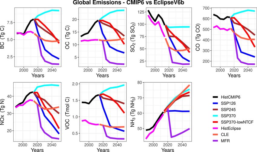
10418                                               U. Im et al.: Present and future aerosol impacts on Arctic climate change

Figure 1. Global recent past and future CMIP6 and Eclipse V6b anthropogenic emissions for different pollutants and scenarios.

Table 1. GISS-E2.1 simulations carried out in the Eclipse and CMIP6 ensembles.

              Simulations                         Description                               No. of ensemble         Period
              NINT_Cpl                            No tracers – coupled                                    1    1850–2014
              Eclipse_AMIP                        AMIP OMA                                                1    1995–2014
              Eclipse_AMIP_NCEP                   AMIP OMA – winds nudged to NCEP                         1    1995–2014
              Eclipse_CplHist                     OMA – coupled                                           3    1990–2014
              Eclipse_Cpl_CLE                     OMA – coupled                                           3    2015–2050
              Eclipse_Cpl_MFR                     OMA – coupled                                           3    2020–2050
              CMIP6_Cpl_Hist                      OMA – coupled                                           1    1850–2014
              CMIP6_Cpl_SSP1-2.6                  OMA – coupled                                           1    2015–2050
              CMIP6_Cpl_SSP2-4.5                  OMA – coupled                                           1    2015–2050
              CMIP6_Cpl_SSP3-7.0                  OMA – coupled                                           1    2015–2050
              CMIP6_Cpl_SSP3-7.0-lowNTCF          OMA – coupled                                           1    2015–2050

sea-ice extent, cloud fraction, and liquid and ice water con-          Arctic stations are Fairbanks and Utqiagvik, Alaska (part of
tent in 1995–2014 period. The surface monitoring stations              IMPROVE, though their measurements were obtained from
used to evaluate the simulated aerosol levels have been listed         their PIs); Gruvebadet and Zeppelin mountain (Ny-Ålesund),
in Tables S1 and S2 in the Supplement.                                 Norway; Villum Research Station, Greenland; and Alert,
                                                                       Nunavut (with the latter being an observatory in the Global
2.4.1   Aerosols                                                       Atmosphere Watch Programme of the WMO and a part of
                                                                       CABM). The measurement techniques are briefly described
Measurements of speciated particulate matter (PM), BC,                 in the Supplement.
SO2−4 , and (OA) come from three major networks: the Inter-
                                                                          AOD at 500 nm from the AErosol RObotic NETwork
agency Monitoring of Protected Visual Environments (IM-                (AERONET, Holben et al., 1998) was interpolated to 550 nm
PROVE) for Alaska (the IMPROVE measurements that are                   AOD using the Ångström formula (Ångström, 1929). We
in the Arctic (> 60◦ N) are all in Alaska), the European Mon-          also used a new merged AOD product developed by So-
itoring and Evaluation Programme (EMEP) for Europe, and                gacheva et al. (2020) using AOD from 10 different satellite-
the Canadian Aerosol Baseline Measurement (CABM) for                   based products. According to Sogacheva et al. (2020), this
Canada (Tables S1 and S2). In addition to these monitoring             merged product could provide a better representation of tem-
networks, BC, OA, and SO2−   4 measurements from individ-
                                                                       poral and spatial distribution of AOD. However, it is impor-
ual Arctic stations were used in this study. The individual            tant to note that the monthly aggregates of observations for

Atmos. Chem. Phys., 21, 10413–10438, 2021                                               https://doi.org/10.5194/acp-21-10413-2021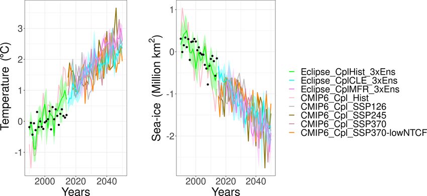
U. Im et al.: Present and future aerosol impacts on Arctic climate change                                                10419

both AERONET and the satellite products depend on avail-            Cloud liquid and ice water path estimates derived from the
ability of data and are not likely to be the true aggregate of   cloud profiling radar aboard CloudSat (Stephens et al., 2002)
observations for a whole month when only few data points         and constrained with another sensor aboard NASA’s A-Train
exist during the course of a month. In addition, many polar-     constellation, MODIS-Aqua (Platnick et al., 2015), are used
orbiting satellites take one observation during any given day    for the model evaluation. These Level 2b retrievals, available
and typically at the same local time. Nevertheless, these        through the 2B-CWC-RVOD product (Version 5), for the
datasets are key observations currently available for evalu-     period 2007–2016 are analyzed. This constrained version
ating model performances. Information about the uncertain        is used instead of its radar-only counterpart, as it uses
nature of AOD observations can be found in previous stud-        additional information about visible cloud optical depths
ies (e.g., Sayer et al., 2018; Sayer and Knobelspiesse, 2019;    from MODIS, leading to better estimates of cloud liquid
Wei et al., 2019; Schutgens et al., 2020, Schutgens, 2020;       water paths. Because of this constraint the data are available
Sogacheva et al., 2020).                                         only for the daylit conditions and, hence, are missing over
                                                                 the polar regions during the respective winter seasons.
2.4.2   Surface air temperature, precipitation, and sea          The theoretical basis for these retrievals can be found at
        ice                                                      http://www.cloudsat.cira.colostate.edu/sites/default/files/
                                                                 products/files/2B-CWC-RVOD_PDICD.P1_R05.rev0_.pdf
Surface air temperature and precipitation observations used      (last access: 26 October 2020). Being an active cloud radar,
in this study are from University of Delaware gridded            CloudSat provides orbital curtains with a swath width of
monthly mean datasets (UDel; Willmott and Matsuura,              just about 1.4 km. Therefore, the data are gridded at 5◦ × 5◦
2001). UDel’s 0.5◦ resolution gridded datasets are based         to avoid too many gaps or patchiness and to provide robust
on interpolations from station-based measurements obtained       statistics.
from various sources including the Global Historical Climate
Network, the archive of Legates and Willmott, and others.
The Met Office Hadley Centre’s sea ice and sea surface tem-      3     Results
perature (HadISST; Rayner et al., 2003) was used for evaluat-
ing model simulations of sea ice and SSTs. HadISST data are      3.1     Evaluation
an improved version of their predecessor known as global sea
ice and sea surface temperature (GISST). HadISST data are        The simulations are compared against surface measurements
constructed using information from a variety of data sources     of BC, OA, SO2− 4 , and AOD, as well as surface and satel-
such as the Met Office marine database, International Com-       lite measurements of surface air temperature, precipitation,
prehensive Ocean-Atmosphere Data Set, passive microwave          sea surface temperature, sea-ice extent, total cloud fraction,
remote sensing retrieval, and sea-ice charts.                    liquid water path, and ice water path described in Sect. 2.4,
                                                                 by calculating the correlation coefficient (r) and normalized
2.4.3   Satellite observations used for cloud fraction and       mean bias (NMB). OA refers to the sum of primary organic
        cloud liquid water and ice water                         carbon (OC) and secondary organic aerosol (SOA).

The Advanced Very High Resolution Radiometer (AVHRR-             3.1.1    Aerosols
2) sensors aboard the NOAA and EUMETSAT polar-orbiting
satellites have been flying since the early 1980s. These data    The recent past simulations are for BC, OA, SO4 , and
have been instrumental in providing the scientific commu-        AOD (Table 2) against available surface measurements. The
nity with climate data records spanning nearly four decades.     monthly observed and simulated time series for each station
Tremendous progress has been made in recent decades in           are accumulated per species in order to get full Arctic time
improving, training, and evaluating the cloud property re-       series data, which also include spatial variation, to be used
trievals from these AVHRR sensors. In this study, we use         for the evaluation of the model. In addition to Table 2, the
the retrievals of total cloud fraction from the second edi-      climatological mean (1995–2014) of the observed and simu-
tion of EUMETSAT’s Climate Monitoring Satellite Appli-           lated monthly surface concentrations of BC, OA, SO2−    4 , and
cation Facility (CM SAF) Cloud, Albedo and surface Radia-        AOD at 550 nm (note that AOD is averaged over 2008, 2009,
tion dataset from AVHRR data (CLARA-A2, Karlsson et al.,         and 2014) is shown in Fig. 2. The AOD observation data for
2017a). This cloud property climate data record is available     years 2008, 2009, and 2014 are used in order to keep the
for the period 1982–2018. Its strengths and weaknesses, and      comparisons in line with the multi-model evaluations being
inter-comparison with the other similar climate data records     carried out in the AMAP assessment report (AMAP, 2021).
are documented in Karlsson and Devasthale (2018). Further        We also provide spatial distributions of the NMB, calculated
dataset documentation including algorithm theoretical ba-        as the mean of all simulations for BC, OA, SO4 , and AOD in
sis and validation reports can be found in Karlsson et al.       Fig. 3. The statistics for the individual stations are provided
(2017b).                                                         in Tables S3–S6 in the Supplement.

https://doi.org/10.5194/acp-21-10413-2021                                        Atmos. Chem. Phys., 21, 10413–10438, 2021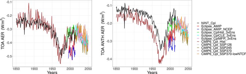
10420                                                   U. Im et al.: Present and future aerosol impacts on Arctic climate change

Table 2. Annual mean normalized mean bias (NMB: %) and correlation coefficients (r) for the recent past simulations in the GISS-E2.1
model ensemble during 1995–2014 for BC, OA, SO2−
                                              4 , and 2008/09–2014 for AOD550 from AERONET and satellites.

                                            BC                  OA                SO2−
                                                                                    4             AOD_aero            AOD_sat
         Model                          NMB         r       NMB        r       NMB         r     NMB           r    NMB         r
         AMAP_OnlyAtm                 −67.32     0.27      −35.46    0.54     −49.83     0.65   −33.28    −0.07     −0.48    0.00
         AMAP_OnlyAtm_NCEP            −57.00     0.26       −7.80    0.56     −52.70     0.74   −41.99     0.02     −0.55    0.13
         AMAP_CplHist (x3)            −64.11     0.42      −19.07    0.58     −49.39     0.71   −43.28     0.04     −0.56    0.07
         CMIP6_Cpl_Hist               −49.90     0.26       13.14    0.69     −39.81     0.70   −39.86     0.05     −0.53    0.11

Figure 2. Observed and simulated Arctic climatological (1995–2014) monthly BC, OA, SO2−   4 , and AERONET AOD at 550 nm (2008/09–
2014), along with the interannual variation shown in bars. The data present monthly accumulated time series for all stations that are merged
together.

   Results showed overall an underestimation of aerosol                    ularly for the Northern Hemisphere winter months, with the
species over the Arctic, as discussed below. Surface BC lev-               largest model diversity near natural emission source regions
els are underestimated at all Arctic stations from 15 % to                 and the polar regions.
90 %. Surface OA levels are also underestimated from −5 %                     The BC levels are largely underestimated in simulations
to −70 %, except for a slight overestimation of < 1 % over                 by 50 % (CMIP6_Cpl_Hist) to 67 % (Eclipse_AMIP). The
Kårvatn (B5) and a large overestimation of 90 % over Trap-                 CMIP6 simulations have lower bias compared to Eclipse
per Creek (B6). Surface SO2− 4 concentrations are also con-                V6b simulations due to higher emissions in the CMIP6
sistently underestimated from −10 % to −70 %, except for                   emission inventory (Fig. 1). Within the Eclipse V6b sim-
Villum Research Station (S11) over northeastern Greenland                  ulations, the lowest bias (−57 %) is calculated for the
where there is an overestimation of 45 %. Finally, AODs                    Eclipse_AMIP_NCEP simulation, while the free climate and
are also underestimated over all stations from 20 % to 60 %.               coupled simulations showed a larger underestimation (>
Such underestimations at high latitudes have also been re-                 62 %), which can be attributed to a better simulation of
ported by many previous studies (e.g., Skeie et al., 2011;                 transport to the Arctic when nudged winds are used. The
Eckhardt et al., 2015; Lund et al., 2017, 2018; Schacht et                 Eclipse simulations also show that the coupled simulations
al., 2019; Turnock et al., 2020), pointing to a variety of rea-            had slightly smaller biases (NMB = −63 %) compared to
sons including uncertainties in emission inventories, errors               the AMIP-type free climate simulation (AMIP-OnlyAtm:
in the wet and dry deposition schemes, the absence or under-               NMB = −67 %). The climatological monthly variation of
representation of new aerosol formation processes, and the                 the observed levels is poorly reproduced by the model with
coarse resolution of global models leading to errors in emis-              r values around 0.3. BC levels are mainly underestimated
sions and simulated meteorology, as well as in representation              in winter and spring, which can be attributed to the under-
of point observations in coarse model grid cells. Turnock et               estimation of the anthropogenic emissions of BC, while the
al. (2020) evaluated the air pollutant concentrations in the               summer levels are well captured by the majority of the sim-
CMIP6 models, including the GISS-E2.1 ESM, and found                       ulations (Fig. 2).
that observed surface PM2.5 concentrations are consistently                   Surface OA concentrations are underestimated from 8 %
underestimated in CMIP6 models by up to 10 µg m−3 , partic-                (Eclipse_AMIP_NCEP) to 35 % (Eclipse_AMIP) by the

Atmos. Chem. Phys., 21, 10413–10438, 2021                                                  https://doi.org/10.5194/acp-21-10413-2021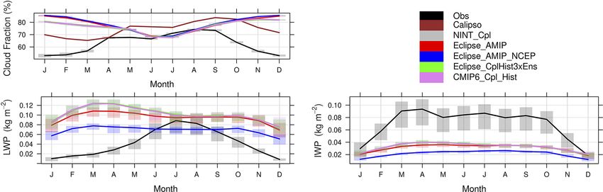
U. Im et al.: Present and future aerosol impacts on Arctic climate change                                                   10421

Figure 3. Spatial distribution of normalized mean bias (NMB, in %) for climatological mean (1995–2014) BC, OA, SO2−
                                                                                                                 4 , and AOD at
monitoring stations, calculated as the mean of all recent past simulations.

Eclipse ensemble, while the CMIP6_Cpl_Hist simulation             sources for the summertime aerosol levels over the Arctic
overestimated surface OA by 13 %. The Eclipse simulations         (Orellana et al., 2011; Karl et al., 2013; Schmale et al., 2021).
suggest that the nudged winds lead to a better representation        Surface SO2−  4   levels are simulated with a smaller
of transport to the Arctic, while the coupled simulations had     bias compared to the BC levels; however, they are
smaller biases compared to the AMIP-type free climate sim-        still underestimated by 40 % (CMIP6_Cpl_Hist) to 53 %
ulation (AMIP-OnlyAtm), similar to BC. The climatological         (Eclipse_AMIP_NCEP). The Eclipse_AMIP_NCEP simu-
monthly variation of the observed concentrations are reason-      lation is biased higher (NMB = −53 %) compared to the
ably simulated, with r values between 0.51 and 0.69 (Table 2      Eclipse_AMIP (NMB = −50 %), probably due to higher
and Fig. 2). As can be seen in Fig. S1, the OA levels are         cloud fraction simulated by the nudged version (see
dominated by the biogenic SOA, in particular via α-pinene         Sect. 3.1.6), leading to higher in-cloud SO2−4 production. The
(monoterpenes) oxidation, compared to anthropogenic (by a         climatological monthly variation of observed SO2−   4 concen-
factor of 4–9) and biomass burning (by a factor of 2–3) OA.       trations is reasonably simulated in all simulations (r = 0.65–
While OC and BC are emitted almost from similar sources,          0.74). The observed springtime maximum is well captured by
this biogenic-dominated OA seasonality also explains why          the GISS-E2.1 ensemble, with underestimations in all sea-
simulated BC seasonality is not as well captured, suggest-        sons, mainly suggesting underestimations in anthropogenic
ing the underestimations in the anthropogenic emissions of        SO2 emissions (Fig. 2), as well as simulated cloud fractions,
these species, in particular during the winter. It should also    which have high positive bias in winter and transition sea-
be noted that GISS-E2.1 does not include marine VOC emis-         sons, while in summer the cloud fraction is well captured
sions except for DMS, while these missing VOCs such as            with a slight underestimation. The clear-sky AOD over the
isoprene and monoterpenes are suggested to be important           AERONET stations in the Arctic region is underestimated
                                                                  by 33 % (Eclipse_AMIP) to 47 % (Eclipse_CplHist1). Simi-

https://doi.org/10.5194/acp-21-10413-2021                                       Atmos. Chem. Phys., 21, 10413–10438, 2021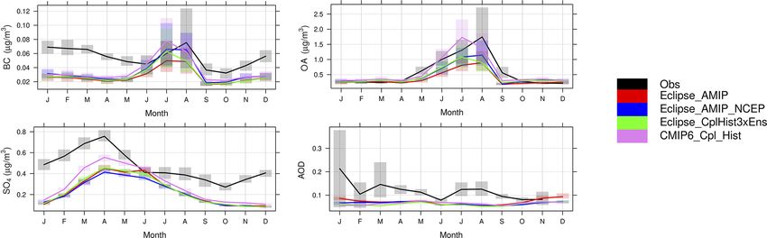
10422                                            U. Im et al.: Present and future aerosol impacts on Arctic climate change

lar negative biases are found with comparison to the satellite   lated by the atmosphere-only simulations, with the nudged
based AOD product (Table 2). The climatological monthly          simulation having the largest bias (NMB = 25 %). The cou-
variation is poorly captured with r values between −0.07 and     pled model simulations are closer to the observations dur-
0.07 compared to AERONET AOD and between 0 and 0.13              ing the recent past. On the other hand, the climatology of
compared to satellite AOD. The simulations could not rep-        the annual-mean cloud fraction was best simulated by the
resent the climatological monthly variation of the observed      nudged atmosphere-only simulation (Eclipse_AMIP_NCEP)
AERONET AODs (Fig. 2).                                           with an r value of 0.40, while other simulations showed
                                                                 a poor performance (r = −0.17 to +0.10), except for the
3.1.2   Climate                                                  summer where the bias is lowest (Fig. 5). The evaluation
                                                                 against CALIPSO data however shows much smaller biases
The different simulations are evaluated against a set of cli-    (NMB = +3 % to +6 %). This is because in comparison to
mate variables, and the statistics are presented in Table 3a     the CALIPSO satellite that carries an active lidar instrument
and b and in Figs. 4 and 5. The climatological mean (1995–       (CALIOP), the CLARA-A2 dataset has difficulties in sepa-
2014) monthly Arctic surface air temperatures are slightly       rating cold and bright ice/snow surfaces from clouds, thereby
overestimated by up to 0.55 ◦ C in the AMIP simulations,         underestimating the cloudiness during Arctic winters. Here
while the coupled ocean simulations underestimate the sur-       both datasets are used for the evaluation as they provide dif-
face air temperatures by up to −0.17 ◦ C. All simulations        ferent observational perspectives and cover the typical range
were able to reproduce the monthly climatological variation      of uncertainty expected from the satellite observations. Fur-
with r values of 0.99 and higher (Fig. 4). Results show that     thermore, while the CLARA-A2 covers the entire evaluation
both absorbing (BC) and scattering aerosols (OC and SO2−   4 )   period in current climate scenario, CALIPSO observations
are underestimated by the GISS-E2.1 model, implying that         are based on 10-year data covering the 2007–2016 period.
these biases can partly cancel out their impacts on radiative       Figure 5 shows the evaluation of the simulations with re-
forcing due to aerosol–radiation interactions. This, together    spect to LWP and IWP. It has to be noted here that to obtain
with the very low biases in surface temperatures, suggests       a better estimate of the cloud water content, the CloudSat
that the effects of the anthropogenic aerosols on the Arctic     observations were constrained with MODIS observations,
climate via radiation are not the main driver in comparison      which resulted in a lack of data during the months with
to cloud indirect effects and forcing from greenhouse gases.     darkness (October–March) over the Arctic (see Sect. 2.4.3).
The monthly mean precipitation has been underestimated by        Hence, we present the results for the polar summer months
around 50 % by all simulations (Table 3a), with the largest      only. As seen in Fig. 5, all simulations overestimated the cli-
biases during the summer and autumn (Fig. 4). The observed       matological (2007–2014) mean polar summer LWP by up to
monthly climatological mean variation was very well simu-        almost 75 %. The smallest bias (14 %) is calculated for the
lated by all simulations, with r values between 0.80 and 0.90.   nudged atmosphere only (Eclipse_OnlyAtm_NCEP), while
   Arctic SSTs are underestimated by the ocean-coupled sim-      the coupled simulations had biases of 70 % or more. Obser-
ulation up to −1.96 ◦ C, while the atmosphere-only runs          vations show a gradual increase in the LWP, peaking in July,
underestimated SSTs by −1.5 ◦ C (Table 3a). The negative         whereas the model simulates a more constant amount for
bias in atmosphere-only simulations is due to the different      the nudged simulation and a slightly decreasing tendency for
datasets used to drive the model, which is a combined prod-      the other configurations. All model simulations overestimate
uct of HadISST and NOAA-OI2 (Reynolds et al., 2002), and         LWP during the spring months. The atmosphere-only nudged
to evaluate the model (Rayner et al., 2003), which is only       simulations tend to better simulate the observed LWP dur-
HadISST. The monthly climatological mean variation is well       ing the summer months (June through September). The cou-
captured with r values above 0.99 (Table 3a, Fig. 4), with       pled simulations, irrespective of the emission dataset used,
a similar cold bias in almost all seasons. The sea-ice extent    are closer to observations only during the months of July and
was overestimated by all coupled simulations by about 12 %,      August.
while the AMIP-type Eclipse simulations slightly underesti-         The climatological (2007–2014) mean polar summer IWP
mated the extent by 3 % (Table 3a). The observed variation       is slightly better simulated compared to the LWP, with bi-
was also very well captured with very high r values. The         ases within −60 % with the exception of the nudged Eclipse
winter and spring biases were slightly higher compared to        (Eclipse_AMIP_NCEP) simulation (NMB = −74 %). All
the summer and autumn biases (Fig. 4).                           simulations simulated the monthly variation well, with r val-
   All simulations overestimate the climatological (1995–        ues of 0.95 and more. In the Arctic, the net cloud forcing at
2014) mean total cloud fraction by 21 % to 25 % during the       the surface changes sign from positive to negative during the
extended winter months (October through February), where         polar summer (Kay and L’Ecuyer, 2013). This change typi-
the simulated seasonality is anti-correlated in comparison to    cally occurs in May driven mainly by shortwave cooling at
AVHRR CLARA-A2 observations, whereas a good correla-             the surface. Since the model simulates the magnitude of the
tion is seen during the summer months irrespective of the        LWP reasonably, particularly in summer, the negative cloud
observational data reference. The largest biases were simu-      forcing can also be expected to be realistic in the model (e.g.,

Atmos. Chem. Phys., 21, 10413–10438, 2021                                        https://doi.org/10.5194/acp-21-10413-2021
U. Im et al.: Present and future aerosol impacts on Arctic climate change 10423
Table 3. (a) Annual normalized mean biases (NMB: %) and correlation coefficients (r) for the recent past simulations in the GISS-E2.1 model
ensemble in 1995–2014 for surface air temperature (Tsurf ) and sea surface temperature (SST) in units of degree Celsius (◦ C), precipitation
(Precip), and sea-ice fraction (Sea ice). (b) Annual mean normalized mean biases (NMB: %) and correlation coefficients (r) for the recent
past simulations in the GISS-E2.1 model ensemble in 1995–2014 for total cloud fraction (Cld Frac), liquid water path (LWP), and ice water
path (IWP) in units of percent (%).
(a) Tsurf Precip SST Sea ice (b) Cld Frac LWP IWP
Model NMB r NMB r NMB r NMB r NMB r NMB r NMB r
NINT −0.08 1.00 −52.68 0.88 −88.87 0.99 12.14 1.00 20.95 −0.67 70.55 −0.89 −56.06 0.53
AMAP_OnlyAtm −19.73 1.00 −50.33 0.89 −68.00 0.99 −2.56 1.00 23.78 −0.81 57.52 −0.96 −58.53 −0.18
AMAP_OnlyAtm_NCEP −14.74 1.00 −53.19 0.90 −68.00 0.99 −2.56 1.00 24.83 −0.79 14.19 −0.91 −70.32 −0.64
AMAP_CplHistx3 −3.35 1.00 −53.06 0.86 −87.51 0.99 11.35 1.00 21.64 −0.65 70.99 −0.91 −55.74 0.48
CMIP6_Cpl_Hist −1.22 1.00 −53.96 0.85 −88.53 0.98 12.56 0.99 21.49 −0.65 69.18 −0.91 −56.28 0.40
Figure 4. Observed and simulated Arctic climatological (1995–2014) surface air temperature, precipitation, sea surface temperature, and
sea ice, along with the interannual variation shown in bars. Obs denotes the UDel dataset for surface air temperature and precipitation, and
HadISST denotes that for sea surface temperature and sea-ice extent. Note that the two AMIP runs (blue and red lines) for the SST and sea
ice are on top of each other as they use that data to run as input.
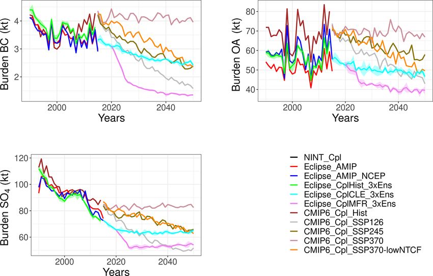
Gryspeerdt et al., 2019). Furthermore, the aerosol and pol- while the OA burden remains relatively constant, although
lution transport into the Arctic typically occurs in the low- there is large year-to-year variability in all simulations. All
ermost troposphere where liquid water clouds are prevalent figures show a decrease in burdens after 2015, except for
during late spring and summer seasons (Stohl, 2006; Law the SSP3-7.0 scenario, where the burdens remain close to
et al., 2014; M. A. Thomas et al., 2019). The interaction of the 2015 levels. The high variability in BC and OA burdens
ice clouds with aerosols is, however, more complex, as ice over the 2000s is due to the biomass burning emissions from
clouds could have varying optical thicknesses, with mainly the Global Fire Emissions Database (GFED), which have not
thin cirrus in the upper troposphere and relatively thicker been harmonized with the no-satellite era. It should also be
clouds in the layers below. Without the knowledge on the noted that these burdens can be underestimated considering
vertical distribution of optical thickness, it is difficult to infer the negative biases calculated for the surface concentrations
the potential impact of the underestimation of IWP on total and in particular for the AODs reported in Tables 2 and S2–
cloud forcing and their implications. S6.
In addition to the burdens of these aerosol species, the
3.2 Arctic burdens and radiative forcing due to TOA radiative forcing due to aerosol–radiation interaction
aerosol–radiation interactions (RFARI ) (RFARI ) over the Arctic is simulated by the GISS-E2.1 en-
semble. RFARI is calculated as the sum of shortwave and
The recent past and future Arctic column burdens for BC, longwave forcing from the individual aerosol species be-
OA, and SO2− tween 1850 and 2050 is presented in Fig. 7. It is important to
4 for the different scenarios and emissions are
provided in Fig. 6. In addition, Table 4 shows the calculated note that the present study uses the instantaneous forcing di-
trends in the burdens for BC, OA, and SO2− agnostics from the model, which are calculated with a double
4 for the dif-
ferent scenarios, while Table 5 provides the 1990–2010 and call to the model’s radiation code, with and without aerosols,
2030–2050 mean burdens of the aerosol components. The as described in Bauer et al. (2020) and Miller et al. (2021),
BC and SO2− and not the effective radiative forcing. The transient cloud ra-
4 burdens started decreasing from the 1990s,
https://doi.org/10.5194/acp-21-10413-2021 Atmos. Chem. Phys., 21, 10413–10438, 202110424 U. Im et al.: Present and future aerosol impacts on Arctic climate change
Figure 5. Observed and simulated Arctic climatological total cloud fraction (1995–2014 mean), liquid water path (2007–2014 mean), and
ice water path (2007–2014 mean), along with the interannual variation shown in bars. Obs denote CLARA-A2 for the cloud fractions and
CloudSat for the LWP and IWP.
Figure 6. Arctic BC, OA, and SO2−
4 burdens in 1990–2050 as calculated by the GISS-E2.1 ensemble.
diative effect in GISS-E.2.1 follows Ghan (2013), which cal- ulations in the CMIP6 ensemble, where the anthropogenic
culates the difference in cloud radiative forcing with aerosol RFARI by NINT simulation is less negative (by almost 30 %)
scattering and absorption omitted (Bauer et al., 2020). How- compared to the OMA simulation (Fig. 7b). On the other
ever, the present study only focuses on the RFARI . The model hand, no such difference is seen in the net RFARI time series
outputs separate forcing diagnostics for anthropogenic and (Fig. 7a). This compensation is largely driven by the 50 %
biomass burning BC and OC, as well as biogenic SOA, mak- more positive dust and 10 % less negative sea-salt RFARI in
ing it possible to attribute the forcing to individual aerosol the OMA simulation.
species. The negative RFARI has increased significantly since
1850 until the 1970s due to an increase in aerosol concentra- 3.2.1 Black carbon
tions. Due to the efforts of mitigating air pollution and thus
a decrease in emissions, the forcing became less negative af- All simulations show a statistically significant (as calcu-
ter the 1970s until 2015. Figure 7 also shows a visible dif- lated by Mann–Kendall trend analyses) decrease in the Arc-
ference in the anthropogenic RFARI simulated by the NINT tic BC burdens (Table 4) between 1990–2014, except for the
(prescribed aerosols) and OMA (interactive aerosols) sim- CMIP6_Cpl_Hist, which shows a slight non-significant in-
crease that can be attributed to the large increase in global an-
Atmos. Chem. Phys., 21, 10413–10438, 2021 https://doi.org/10.5194/acp-21-10413-2021U. Im et al.: Present and future aerosol impacts on Arctic climate change 10425
Table 4. Trends in Arctic BC, OA, and SO2−4 burdens in the near past (1990–2014) and future (2030–2050) as calculated by the GISS-E2.1.
The bold numbers indicate the trends that are statistically significant on a 95 % significance level.
BC OA SO2−
4
1990–2014 2015–2050 1990–2014 2015–2050 1990–2014 2015–2050
Eclipse_AMIP −0.026 0.030 −0.886
Eclipse_AMIP_NCEP −0.021 0.112 −0.939
Eclipse_CplHist_3xEns −0.026 −0.006 −1.332
Eclipse_CplCLE_3xEns −0.024 −0.201 −0.143
Eclipse_CplMFR_3xEns −0.043 −0.367 −0.146
CEDS_Cpl_Hist 0.007 0.121 −1.093
CEDS_Cpl_SSP126 −0.068 −0.715 −0.935
CEDS_Cpl_SSP245 −0.047 −0.384 −0.465
CEDS_Cpl_SSP370 −0.004 −0.062 0.027
CEDS_Cpl_SSP370-lowNTCF −0.051 −0.642 −0.567
Table 5. Arctic BC, OA, and SO2−
4 burdens in 1990–2010 and 2030–2050 periods as calculated by the GISS-E2.1.
BC OA SO2−
4
1990–2010 2030–2050 1990–2010 2030–2050 1990–2010 2030–2050
Eclipse_AMIP 3.52 50.70 95.10
Eclipse_AMIP_NCEP 3.49 57.31 93.93
Eclipse_CplHist_3xEns 3.75 55.55 93.59
Eclipse_CplCLE_3xEns 2.58 48.95 63.52
Eclipse_CplMFR_3xEns 1.44 40.39 53.35
CEDS_Cpl_Hist 3.64 67.48 99.11
CEDS_Cpl_SSP126 2.05 50.41 53.99
CEDS_Cpl_SSP245 2.65 59.43 69.71
CEDS_Cpl_SSP370 4.08 68.81 83.26
CEDS_Cpl_SSP370-lowNTCF 2.94 56.05 69.72
thropogenic BC emissions in CMIP6 after year 2000 (Fig. 1). over the Arctic (e.g., Schacht et al., 2019). In the future, the
From 2015 onwards, all future simulations show a statisti- positive BC RFARI generally decreases (Fig. 6) due to lower
cally significant decrease in the Arctic BC burden (Table 4). BC emissions and therefore burdens, except for the SSP3-
The Eclipse CLE ensemble shows a 1.1 kt (31 %) decrease 7.0 scenario, where the BC forcing becomes more positive
in the 2030–2050 mean Arctic BC burden compared to the by 0.05 W m−2 due to increasing BC emissions and burdens.
1990–2010 mean, while the decrease in 2030–2050 mean The changes in the Arctic RFARI in Table 6a follow the Arctic
Arctic BC burden is larger in the MFR ensemble (2.3 kt: burdens presented in Table 5 and emission projections pre-
62 %). In the CMIP6 simulations, the 2030–2050 mean Arc- sented in Fig. 1, leading to largest reductions in BC RFARI
tic BC burdens decrease by 0.70 to 1.59 kt, being largest in simulated in SSP1-2.6 (−0.10 W m−2 ). Similar to the bur-
SSP1-2.6 and lowest in SSP3-7.0-lowNTCF, while the SSP3- dens, the Eclipse CLE and CMIP6 SSP2-4.5 scenarios simu-
7.0 simulation leads to an increase of 0.43 kt (12 %) in 2030– late a very close decrease in the 2030–2050 mean BC RFARI
2050 mean Arctic BC burdens. It is important to note that of −0.06 and −0.14 W m−2 , respectively.
the change in burden simulated by the Eclipse CLE ensem-
ble (−1.1 kt) is comparable with the change of −1 kt in the 3.2.2 Organic aerosols
SSP2-4.5 scenario, consistent with the projected emission
changes in the two scenarios (Fig. 1). The Eclipse historical ensemble simulate a positive OA
As seen in Table 6, the GISS-E2.1 ensemble calculated a burden trend between 1990 and 2014; however, this trend
BC RFARI of up to 0.23 W m−2 over the Arctic, with both is not significant at the 95 % confidence level (Table 4).
CMIP6 and Eclipse coupled simulations estimating the high- The CMIP6_Cpl_Hist simulation gives a larger trend, due
est forcing of 0.23 W m−2 for the 1990–2010 mean (Ta- to a large increase in global anthropogenic OC emissions
ble 6a). This agrees with previous estimates of the BC RFARI in CMIP6 (Fig. 1). The nudged AMIP Eclipse simulation
https://doi.org/10.5194/acp-21-10413-2021 Atmos. Chem. Phys., 21, 10413–10438, 2021You can also read