Regional Production, Updated documentation covering all Regional operational systems and the - ENSEMBLE - Copernicus Atmosphere Monitoring Service
←
→
Page content transcription
If your browser does not render page correctly, please read the page content below
ECMWF COPERNICUS REPORT

Copernicus Atmosphere Monitoring Service

                Regional Production,
                Updated documentation covering all
                Regional operational systems and the
                ENSEMBLE
                Following U1 upgrade, summer 2019

                Issued by: METEO-FRANCE / G. Collin
                Date: 31/10/2019
                Ref:
                CAMS50_2018SC1_D2.0.2-U1_Models_documentation_201910_v1
This document has been produced in the context of the Copernicus Atmosphere Monitoring Service (CAMS).
The activities leading to these results have been contracted by the European Centre for Medium-Range Weather Forecasts,
operator of CAMS on behalf of the European Union (Delegation Agreement signed on 11/11/2014). All information in this
document is provided "as is" and no guarantee or warranty is given that the information is fit for any particular purpose.
The user thereof uses the information at its sole risk and liability. For the avoidance of all doubts, the European Commission
and the European Centre for Medium-Range Weather Forecasts has no liability in respect of this document, which is merely
representing the authors view.
Copernicus Atmosphere Monitoring Service

Table of Contents

Executive summary                                                                       5

1. ENSEMBLE factsheet                                                                   6
1.1 Assimilation and forecast system: synthesis of the main characteristics             6
1.2 ENSEMBLE background information                                                     6

2. CHIMERE factsheet                                                                    9
2.1 Assimilation and forecast system: synthesis of the main characteristics            9
2.2 Forward model                                                                      9
2.3 Assimilation system                                                               12

3. EMEP factsheet                                                                     14
3.1 Assimilation and forecast system: synthesis of the main characteristics           14
3.2 Forward model                                                                     15
3.3 Assimilation system                                                               18

4. EURAD-IM factsheet                                                                 19
4.1 Assimilation and forecast system: synthesis of the main characteristics           19
4.2 Forward model                                                                     20
4.3 Assimilation system                                                               24

5. LOTOS-EUROS factsheet                                                              26
5.1 Assimilation and forecast system: synthesis of the main characteristics           26
5.2 Forward model                                                                     27
5.3 Assimilation system                                                               30

6. MATCH factsheet                                                                    31
6.1 Assimilation and forecast system: synthesis of the main characteristics           31
6.2 Forward model                                                                     32
6.3 Assimilation system                                                               35

7. MOCAGE factsheet                                                                   37
7.1 Assimilation and forecast system: synthesis of the main characteristics           37
7.2 Forward model                                                                     38
7.3 Assimilation system                                                               41

8. SILAM factsheet                                                                    42
8.1 Assimilation and forecast system: synthesis of the main characteristics           42

CAMS50_2018SC1 – Updated models’ documentation following U1 upgrade           Page 3 of 78
Copernicus Atmosphere Monitoring Service

8.2 Forward model                                                                      43
8.3 Assimilation system                                                                46

9. DEHM factsheet                                                                      47
9.1 Assimilation and forecast system: synthesis of the main characteristics            47
9.2 Forward model                                                                      48
9.3 Assimilation system                                                                52

10. GEM-AQ factsheet                                                                   53
10.1 Assimilation and forecast system: synthesis of the main characteristics           53
10.2 Forward model                                                                     53
10.3 Assimilation system                                                               58

11. References                                                                         60
11.1 ENSEMBLE                                                                          60
11.2 CHIMERE                                                                           60
11.3 EMEP                                                                              62
11.4 EURAD-IM                                                                          64
11.5 LOTOS-EUROS                                                                       66
11.6 MATCH                                                                             68
11.7 MOCAGE                                                                            70
11.8 SILAM                                                                             71
11.9 DEHM                                                                              73
11.10 GEM-AQ                                                                           75

CAMS50_2018SC1 – Updated models’ documentation following U1 upgrade            Page 4 of 78
Copernicus Atmosphere Monitoring Service

Executive summary

The Copernicus Atmosphere Monitoring Service (CAMS, atmosphere.copernicus.eu/) is establishing
the core global and regional atmospheric environmental service delivered as a component of Europe's
Copernicus programme. The Regional forecasting service (CAMS_50) currently provides daily 4-day
forecasts of the main air quality species and analyses of the day before, as well as posteriori re-
analyses using the latest validated observation dataset available for assimilation. Since the U1
upgrade performed in summer 2019, 9 state-of-the-art atmospheric chemistry models take part in
the operation production. A median ENSEMBLE is calculated from the 9 model outputs, since
ensemble products generally yield better performance than the individual model products.

Following the U1 upgrade of summer 2019, this document provides an updated description of the 9
operational models contributing to the ENSEMBLE, and also the method used for the ENSEMBLE
production. The 2 additional models that joined operational production on 16/10/2019 (U1.2
upgrade) are also included. For each system, the main components of the model are specified:
chemistry schemes, aerosol representation, emissions and deposition, resolved and sub-grid
transport, boundary conditions, assimilation system. The document is helpful to identify the
differences and common features between the models. It may be used as a reference information
regarding the CAMS Regional operational production.

CAMS50_2018SC1 – Updated models’ documentation following U1 upgrade                      Page 5 of 78
Copernicus Atmosphere Monitoring Service

1. ENSEMBLE factsheet

1.1 Assimilation and forecast system: synthesis of the main characteristics

 ENSEMBLE forecasts and analyses
 Horizontal resolution                                      0.1° regular lat-lon grid
 Domain                                                     25°W-45°E, 30°N-70°N
 ENSEMBLE method                                            Median model: for each grid-cell, the value
                                                            corresponds to the median of the different model
                                                            values
 Individual models                                          Aerosol-uptake of HNO3, HO2 and O3 (EMEP, 2015)

1.2 ENSEMBLE background information

Based on a sample of individual model members, the ensemble approach is useful and relevant for
air quality monitoring (Galmarini et al, 2004). The ensemble products, indeed, generally yield better
performance than the individual model products. Besides, the spread between the different members
may be used to provide some information about the uncertainty of the ensemble products.
Consequently, the forecasts, analyses and re-analyses delivered as part of the CAMS Regional
production are based on an ensemble approach.

1.2.1 Method

The ENSEMBLE is currently based upon a median value approach (Marécal et al, 2015).

For each time step of the daily forecasts, the different individual model fields (see 1.2.2) are
interpolated on a common regular 0.1°x0.1° grid over the European domain (25°W-45°E, 30°N-70°N)
used for the CAMS Regional production. For each point of this grid, the ENSEMBLE model value is
simply defined as the median value of all the individual models’ forecasts on this point. The median
is defined as the value having 50% of individual models with higher values and 50% with lower values.

This method provides an optimal estimate in the statistical sense (Riccio et al, 2007) and is rather
insensitive to outliers in the forecasts, which is a useful property for the quality and for the reliability
of the CAMS Regional production. The method is also little sensitive if a particular model forecast is
occasionally missing.

1.2.2 Individual models

The ENSEMBLE production is based on the 9 individual models listed in Table 1 next page.

CAMS50_2018SC1 – Updated models’ documentation following U1 upgrade                                  Page 6 of 78
Copernicus Atmosphere Monitoring Service
Table 1. Individual models contributing to the ENSEMBLE
Model names Institutes
CHIMERE INERIS (France)
EMEP MET Norway (Norway)
EURAD-IM FZJ-IEK8 (Germany)
LOTOS-EUROS KNMI, TNO (The Netherlands)
MATCH SMHI (Sweden)
MOCAGE Meteo-France (France)
SILAM FMI (Finland)
DEHM AARHUS UNIVERSITY (Denmark)
GEM-AQ IEP-NRI (Poland)
DEHM and GEM-AQ take part in operational production since the U1.2 upgrade of 16/10/2019. In
addition, 2 candidate models will be evaluated over the course of CAMS_50.II for a possible future
integration in the ENSEMBLE: MINNI (ENEA, Italy) and MONARCH (BSC, Spain).
The main characteristics of the individual models are outlined in half-yearly development reports, as
well as in the present document that is regularly updated and available from the CAMS website1. The
latter also provides access to quarterly NRT production reports2 comprising, per model, a description
of the daily analysis and forecast activities undertaken by the models and a performance review.
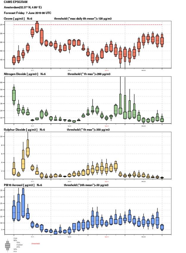
1.2.3 Air quality NRT EPSgrams
Daily, “EPSgrams” for 67 major European cities and urban areas are produced and displayed on the
CAMS website for Regional Air Quality. Such graphics are common for presenting ensemble
meteorological forecast products but, to our knowledge, this is the first experimental implementation
worldwide in the field of Air Quality, which started within the GEMS project.
Figure 1 presents an example of AQ EPSgram. For the 4 main pollutants (ozone, NO2, SO2 and PM10)
forecasts are plotted every 3 hours as bars, which indicate the range of forecasts of individual
ensemble members (minimum, maximum and percentiles 10, 25, 50, 75 and 90). This presentation
allows users to assess the dispersion within the ensemble for each species and each 3-hourly forecast
horizon at the given location of the EPSgram.
The 67 selected sites include the 41 European capitals and 26 urban areas that are among the most
populated ones and where pollution episodes are common. The forecasts are based upon models
that have resolutions of ~10km to 25km, which is too coarse to account for very local and urban
effects (high primary pollutants, titration of ozone, etc.). The AQ EPSgrams presented have thus to be
1
https://atmosphere.copernicus.eu/documentation-regional-systems
2
https://atmosphere.copernicus.eu/validation-regional-systems
CAMS50_2018SC1 – Updated models’ documentation following U1 upgrade Page 7 of 78Copernicus Atmosphere Monitoring Service taken with caution; the forecast does not correspond to city centre values, but rather to values representative of the background in the urban area around the city. Figure 1 - Example of air quality EPSgram at the location of the city of Amsterdam (the Netherlands), concerning June 7th, 2019. CAMS50_2018SC1 – Updated models’ documentation following U1 upgrade Page 8 of 78
Copernicus Atmosphere Monitoring Service

2. CHIMERE factsheet

2.1 Assimilation and forecast system: synthesis of the main characteristics

 Assimilation and forecast system
 Horizontal resolution                                      0.1°x0.1°
 Vertical resolution                                        Variable, 9 levels from the surface up to 500 hPa; 7
                                                            levels below 2 km
 Gas phase chemistry                                        MELCHIOR2, comprising 44 species and 120
                                                            reactions (Derognat, 2003)
 Heterogeneous chemistry                                    NO2, HNO3, N2O5
 Aerosol size distribution                                  10 bins from 10 nm to 40 μm
 Inorganic aerosols                                         Primary particle material, nitrate, sulphate,
                                                            ammonium
 Secondary organic aerosols                                 Biogenic, anthropogenic
 Aqueous phase chemistry                                    Sulphate
 Dry deposition/sedimentation                               Classical resistance approach
 Mineral dust                                               Dusts are considered coming from BC and emitted
                                                            by desert area inside the domain
 Sea Salt                                                   Inert sea salt
 Boundary values                                            Values provided by CAMS global
 Initial values                                             24h forecast from the day before
 Anthropogenic emissions                                    CAMS-REG-AP_v2.2.1 - 2015
 Biogenic emissions                                         MEGAN
 Forecast system
 Meteorological driver                                      00:00 UTC operational IFS forecast from the day
                                                            before
 Assimilation system
 Assimilation method                                        Kriging-based analysis
 Observations                                               Surface ozone, NO2, PM10 and PM2.5
 Frequency of assimilation                                  Every hour over the day before
 Meteorological driver                                      00:00 UTC operational IFS forecast for the day
                                                            before

2.2 Forward model

The CHIMERE multi-scale model is primarily designed to produce daily forecasts of ozone, aerosols
and other pollutants, and to make long-term simulations for emission control scenarios. CHIMERE
runs over a range of spatial scale from the regional scale (several thousand kilometres) to the urban
scale (100-200 Km), with resolutions from 1-2 Km to 100 Km. The chemical mechanism (MELCHIOR)

CAMS50_2018SC1 – Updated models’ documentation following U1 upgrade                                     Page 9 of 78
Copernicus Atmosphere Monitoring Service is adapted from the original EMEP mechanism. Photolytic rates are attenuated using liquid water or relative humidity. Boundary layer turbulence is represented as a diffusion (Troen and Mahrt, 1986, BLM). Vertical wind is diagnosed through a bottom-up mass balance scheme. Dry deposition is as in Wesely (1989). Wet deposition is included. 6 aerosol sizes are represented as bins in the model. Aerosol thermodynamic equilibrium is achieved using the ISORROPIA model. Several aqueous-phase reactions are considered. Secondary organic aerosols formations are considered. Advection is performed by the PPM (Piecewise Parabolic Method) 3d order scheme for slow species. The numerical time solver is the TWOSTEP method. Its use is relatively simple, provided input data is correctly supplied. It can be run with several vertical resolutions, and with a wide range of complexity. It can be run with several chemical mechanisms, simplified or more complete, with or without aerosols. 2.2.1 Model geometry CHIMERE is a Eulerian deterministic model, using variable resolution in time and space (for Cartesian grids). The model uses any number of vertical layers, described in hybrid sigma-p coordinates. The model runs over the CAMS domain with a 0.1°x0.1° resolution and 9 vertical levels, extending from the surface up to 500 hPa. 2.2.2 Forcings and boundary conditions 2.2.2.1 Meteorology Within CAMS, CHIMERE is directly forced by the IFS forecasts from the daily operational products delivered at 00 UTC. 2.2.2.2 Chemistry Boundary conditions can be either "external", or given by a coarse resolution CHIMERE simulation. The CAMS regional forecasts of CHIMERE use the global CAMS production forcing from C-IFS (see Table 2). In case the production is delayed, a back-up forcing is available with a climatology built on 5 years of the MACC/CAMS re-analysis. Use of Sea Salt boundary conditions were suspended in the past due to high overestimation. The corrective approach will be implemented before the end of 2019. CAMS50_2018SC1 – Updated models’ documentation following U1 upgrade Page 10 of 78
Copernicus Atmosphere Monitoring Service

Table 2. The chemical and aerosol species taken from C-IFS and used in CHIMERE

 C-IFS Species                   Coupled to CHIMERE Species
 SO4 (0.06-1.0)                  H2SO4 (bins 3-4-5-6)
 OM (0.06-1.0)                   AnBmP BiA1D BiBmP (bins 3-4-5-6)
 BC (0.06-1.0)                   BCAR (bins 3-4-5-6)
 OM (0.06-1.0)                   OCAR (bins 3-4-5-6)
 DUST1 (0.06-1.1)                DUST (bins 3-4-5-6)
 DUST2 (1.1-1.8)                 DUST (bin 7)
 DUST3 (1.8-40)                  DUST (bins 7-8-9-10)
 C2H6                            C2H6
 CH2O                            HCHO
 CH4                             CH4
 CO                              CO
 HNO3                            HNO3
 ISOP                            C5H8
 NO2                             NO2
 GO3                             O3
 PAN                             PAN
 SO2                             SO2

2.2.2.3 Land use

The proposed domain interface is based on the Global Land Cover Facility (GLCF):
http://glcf.umiacs.umd.edu/data/landcover 1kmx1km resolution database from the University of
Maryland, following the methodology of Hansen et al. (2000, J. Remote Sensing).

2.2.2.4 Surface emissions

The surface emissions are from the TNO emission inventory for anthropogenic emissions. Biogenic
emissions are calculated online with the MEGAN module.
Hourly GFAS Fire emissions are downloaded daily from the dedicated Copernicus service through the
MARS interface, use of ECPDS is under investigation.
Dust emissions are calculated online within CHIMERE.

2.2.3 Dynamical core

3 advection schemes are implemented: the Parabolic Piecewise Method (PPM, a 3-order horizontal
scheme, after Colella and Woodward, 1984), the Godunov scheme (Van Leer, 1979) and the simple
upwind first-order scheme.

CAMS50_2018SC1 – Updated models’ documentation following U1 upgrade                    Page 11 of 78
Copernicus Atmosphere Monitoring Service

2.2.4 Physical parameterisations

2.2.4.1 Turbulence and convection

Vertical turbulent mixing takes place only in the boundary layer. The formulation uses K-diffusion
following the parameterisation of [Troen and Mahrt, 1986], without counter-gradient term.

2.2.4.2 Deposition

Dry deposition is considered for model gas species i and is parameterised as a downward flux F(d,i)=
-v(d,i) c(i) out of the lowest model layer with c(i) being the concentration of species i. As commonly,
the deposition velocity is described through a resistance analogy [Wesely, 1989]. The wet deposition
follows the scheme proposed by [Loosmore, 2004].

2.2.5 Chemistry and aerosols

In order to decrease the computing time, a reduced mechanism with 44 species and about 120
reactions is derived from MELCHIOR [Derognat, 2003], following the concept of chemical operators
[Carter, 1990]. This reduced mechanism is called MELCHIOR2 hereafter.

The CAMS CHIMERE version consists in the baseline gas-phase version with MELCHIOR2 chemistry,
together with a sectional aerosol module. This module accounts for 7 species (primary particle
material, nitrate, sulfate, ammonium, biogenic secondary organic aerosol SOA, anthropogenic SOA
and water). Potentially, chloride and sodium can be included (high computing time). The aerosol
distribution is represented using 9 bins from 10 nm to 10 μm.

2.3 Assimilation system

The CHIMERE assimilation for CAMS relies on a kriging based-approach to assimilate hourly
concentration values for correcting the raw forecasts. This method has been widely evaluated and
validated in the PREV’AIR (Rouïl et al, 2005) system for ozone and PM 10. However, future evolution
of the CHIMERE assimilation system is foreseen to perform multi-pollutant and multi-sensor
assimilation at the same time with a more complex method.

2.3.1 Kriging-based analysis

Several variants of kriging have been tested and compared (Malherbe et al., 2012): kriging of the
innovations (i.e. kriging of CHIMERE errors); kriging with CHIMERE as external drift; ordinary co-
kriging between the observations and CHIMERE.

CAMS50_2018SC1 – Updated models’ documentation following U1 upgrade                         Page 12 of 78
Copernicus Atmosphere Monitoring Service For operational applications, kriging with external drift, which gave the highest scores for ozone (Malherbe and Ung, 2009) and is faster than co-kriging, was found to be the best compromise between efficiency and computing time. It has been implemented in PREV’AIR since 2010, as replacement for kriging of the innovations. It proceeds according to the following steps: Hourly monitoring data are retrieved from CAMS_50. Linear regression between a selected set of observations and CHIMERE is performed (in moving neighbourhood). The experimental variogram of the regression residuals is computed and a variogram model is fitted; the model adequacy is checked by cross validation. Observations are kriged with the CHIMERE model as external drift (in moving neighbourhood). Additional monitoring data, which are not used for calculating the variogram (e.g. data from some mountain sites), are included at this stage. For regulatory applications, the choice of the kriging technique and related parameters is adapted to each pollutant, according to cross-validation and validation tests: For PM10, ordinary co-kriging of the observations (main variable) and CHIMERE (secondary variable) is currently applied. Inclusion of emission density as auxiliary variable and comparison with kriging with external drift are in progress. For NO2, kriging with external drift is performed. CHIMERE, NOx emission density and population density are used as external drift. CAMS50_2018SC1 – Updated models’ documentation following U1 upgrade Page 13 of 78
Copernicus Atmosphere Monitoring Service

3. EMEP factsheet

3.1 Assimilation and forecast system: synthesis of the main characteristics

 Assimilation and forecast system
 Horizontal resolution                                      0.125° x 0.0625° lon-lat (native model grid)
 Vertical resolution                                        20 layers (sigma) up to 100 hPa, with approximately
                                                            10 in the Planetary Boundary layer
 Gas phase chemistry                                        Evolution of the ‘EMEP scheme’, comprising 70
                                                            species and 140 reactions (Andersson-Sköld and
                                                            Simpson, 1999; Simpson et al. 2012)
 Heterogeneous chemistry                                    Aerosol-uptake of HNO3, HO2 and O3 (EMEP, 2015)
 Aerosol size distribution                                  2 size fractions PM2.5 and PM10-2.5
 Inorganic aerosols                                         MARS (Binkowski and Shankar, 1995),
                                                            thermodynamic equilibrium for the
                                                            H+-NH4+-SO42--NO3--H2O system
 Secondary organic aerosols                                 EmChem09soa (Simpson et al., 2012, Bergström et
                                                            al, 2012)
 Aqueous phase chemistry                                    SO2 oxidation by ozone and H2O2 and metal ion-
                                                            catalyzed O2
 Dry deposition/sedimentation                               Resistance approach for gases and for aerosol,
                                                            including non-stomatal deposition of NH3
 Mineral dust                                               Boundary conditions from global C-IFS are used,
                                                            EMEP dust source inside the model domain
 Sea Salt                                                   Boundary conditions from global C-IFS are used
 Boundary values                                            Boundary conditions from global C-IFS are used
 Initial values                                             From end file of D-2 analysis, i.e. valid at D-1, 00UTC
 Anthropogenic emissions                                    TNO-MACC emission data for 2011
 Biogenic emissions                                         Included
 Forecast system
 Meteorological driver                                      12:00 UTC operational IFS forecast (yesterday’s)
 Assimilation system
 Assimilation method                                        Intermittent 3d-var
 Observations                                               NO2 columns from OMI. NO2, O3, SO2, and PM10
                                                            surface concentrations, distributed by Meteo-
                                                            France and INERIS
 Frequency of assimilation                                  Hourly
 Meteorological driver                                      00 UTC operational IFS forecast

CAMS50_2018SC1 – Updated models’ documentation following U1 upgrade                                     Page 14 of 78
Copernicus Atmosphere Monitoring Service 3.2 Forward model The EMEP MSC-W model is a chemical transport model developed at the Norwegian Meteorological Institute under the EMEP programme (UN Convention on Long-range Transboundary Air Pollution). This Eulerian model is developed to be concerned with the regional atmospheric dispersion and deposition of acidifying and eutrophying compounds (S, N), ground level ozone (O 3) and particulate matter (PM2.5, PM10). The EMEP MSC-W model system allows several options with regard to the chemical schemes used and the possibility of including aerosol dynamics. Simpson et al. (2012) describes the EMEP MSC-W model in detail, as well as the main model updates since 2006. The forecast version of the EMEP MSC-W model (EMEP-CWF) is in operation since June 2006. The scheduled model updates in CAMS_50 ensure that the model version stays as close as possible to the official EMEP Open Source version. Nevertheless, the EMEP-CWF results and performances in CAMS_50 might differ from those presented in the annual EMEP Status Reports, because of different input data (emissions and meteorological driver) and model run modes (Forecast in EMEP-CWF versus Hindcast in EMEP Status Reports). 3.2.1 Model geometry The EMEP-CWF covers the European domain [30°N-76°N] x [25°W-45°E] on a geographic projection with a horizontal resolution of 0.125° x 0.0625° (longitude-latitude). Vertically the model uses 20 levels defined as sigma coordinates. The 10 lowest model levels are within the PBL, and the top of the model domain is at 100 hPa. 3.2.2 Forcings and boundary conditions 3.2.2.1 Meteorology 4-day meteorological forecasts from the IFS system of the ECMWF are retrieved daily around 18:15 UTC (12 UTC forecast, used for the EMEP-CWF forecasts) and at 06:15 UTC (00 UTC forecast, used for the EMEP-CWF analyses). The ECMWF forecasts do not include 3D precipitation, which is needed by the EMEP-CWF model. Therefore, a 3D precipitation estimate is derived from large-scale precipitation and convective precipitation (surface variables). Currently the 12 UTC forecast from yesterday’s forecast is used, so that there is sufficient time to run the EMEP-CWF well before the deadline for delivery. 3.2.2.2 Chemistry If available at the start of the forecast run, boundary conditions are taken from the C-IFS. In cases where C-IFS boundary conditions are not available, default boundary conditions are specified for O 3, CO, NO, NO2, CH4, HNO3, PAN, SO2, isoprene, C2H6, some VOCs, Sea salt, Saharan dust and SO4, as CAMS50_2018SC1 – Updated models’ documentation following U1 upgrade Page 15 of 78
Copernicus Atmosphere Monitoring Service

annual mean concentrations along with a set of parameters for each species describing seasonal,
latitudinal and vertical distributions.

Table 3. The chemical and aerosol species taken from C-IFS and used in EMEP. In EMEP ‘F’ stands for the fine
fraction (diameters smaller than 2.5 µm) and ‘C’ stands for the coarse fraction (diameters between 2.5 and 10
µm). The mapping of IFS size bins into EMEP size bins is based on consideration of typical size distributions.
a
  For sea salt a correction factor of 1/4.3 is applied, since C-IFS Sea Salt is calculated for 80% relative humidity
while the EMEP Sea Salt contains only the dry component.

 C-IFS Species                                 Coupled to EMEP Species             Comments
 GO3                                           O3
 CO                                            CO
 NO                                            NO
 NO2                                           NO2
 PAN                                           PAN
 HNO3                                          HNO3
 HCHO                                          HCHO
 SO2                                           SO2
 CH4                                           CH4
 C5H8                                          C5H8
 C2H6                                          C2H6
 aermr01 (sea salt 0.03-0.5 µm)                SEASALT_F (0-2.5 µm)                SEASALT_F=aermr01/4.3 a
 aermr02 (sea salt 0.5-5 µm)                   SEASALT_C (2.5-10 µm)               SEASALT_C=aermr02/4.3 a
 aermr03 (sea salt 5-20 µm)                                                        Not used
 aermr04 (dust 0.03-0.55 µm)                   DUST_SAH_F (0-2.5 µm)
 aermr05 (dust 0.55-0.9 µm)                    DUST_SAH_F (0-2.5 µm)
 aermr06 * 0.15 (dust 0.9-20 µm)               DUST_SAH_F (0-2.5 µm)               15% of aermr06 used
 aermr06 * 0.35 (dust 0.9-20 µm)               DUST_SAH_C (2.5-10 µm)              35% of aermr06 used
 aermr11                                       SO4

3.2.2.3 Surface emissions

The TNO-MACC emission data set for 2011 is used, interpolated on the model’s native grid, i.e. 0.125°
x 0.0625° (lon-lat) resolution. (from June 2019, CAMS-REG-AP_v2.2.1 will be used)

3.2.3 Dynamical core

The numerical solution of the advection terms of the continuity equation is based on the scheme of
(Bott, 1989). The fourth order scheme is utilized in the horizontal directions. In the vertical direction,
a second order version applicable to variable grid distances is employed.

CAMS50_2018SC1 – Updated models’ documentation following U1 upgrade                                     Page 16 of 78
Copernicus Atmosphere Monitoring Service

3.2.4 Physical parameterisations

3.2.4.1 Turbulence and convection

The turbulent diffusion coefficients (Kz) are first calculated for the whole 3D mode domain on the
basis of local Richardson numbers. The planetary boundary layer (PBL) height is then calculated using
methods described in (Simpson et al., 2012). For stable conditions, Kz values are retained. For
unstable situations, new Kz values are calculated for layers below the mixing height using the O'Brien
interpolation (Simpson et al., 2012).

3.2.4.2 Deposition

Parameterisation of dry deposition is based on a resistance formulation, fully described in Simpson
et al. (2012). The deposition module makes use of a stomatal conductance algorithm which was
originally developed for ozone fluxes, but which is now applied to all gaseous pollutants when
stomatal control is important (Emberson et al., 2000; Simpson et al., 2003; Tuovinen et al., 2004).
Non-stomatal deposition for NH3 is parameterised as a function of temperature, humidity, and the
molar ratio SO2/NH3.

3.2.5 Chemistry and aerosols

The chemical scheme couples the sulphur and nitrogen chemistry to the photochemistry using about
140 reactions between 70 species (Andersson-Sköld and Simpson, 1999; Simpson et al. 2012).

The chemical mechanism is based on the ‘EMEP scheme’, as well as reactions to cover acidification,
eutrophication and ammonium chemistry, as described in Simpson et al., 2012 and references
therein.

The standard model version distinguishes 2 size fractions for aerosols, fine aerosol (PM 2.5) and coarse
aerosol (PM2.5-10). The aerosol components presently accounted for are SO4, NO3, NH4, anthropogenic
primary PM and sea salt. Also aerosol water is calculated. Dry deposition parameterisation for
aerosols follows standard resistance-formulations, accounting for diffusion, impaction, interception,
and sedimentation. Wet scavenging is treated with simple scavenging ratios, taking into account in-
cloud and sub-cloud processes. For secondary organic aerosol (SOA) the so-called EmChem09soa
scheme is used, which is a somewhat simplified version of the mechanisms discussed in detail by
Bergström et al. (2012).

CAMS50_2018SC1 – Updated models’ documentation following U1 upgrade                          Page 17 of 78
Copernicus Atmosphere Monitoring Service
3.3 Assimilation system
The EMEP data assimilation system (EMEP-DAS) is based on the 3D-Var implementation for the
MATCH model (Kahnert, 2009). The background error covariance matrix is estimated following the
NMC method (Parrish and Derber, 1992).
In its current stage, the EMEP-DAS is built on top of the EMEP MSC-W model version rv4.5 (Simpson
et al., 2012). The EMEP-DAS is described in detail in Valdebenito B. and Heiberg (2009), Valdebenito
B. et al. (2010) and Valdebenito B. and Tsyro (2012).
The EMEP-DAS delivers analyses of yesterday (driven by the operational IFS forecast of 00UTC of
yesterday) for NO2, using NO2 columns of OMI and in-situ measurements of NO2 surface
concentrations. For ozone, SO2, and PM10, only surface measurements are assimilated. CO surface
observations can be assimilated, but this feature is currently switched off in the operational chain.
EMEP-DAS has been in operation since November 2012, with the following major updates (see also
‘Evolutions in the EMEP suite’):
October 2012: version rv4.1, including DA of NO2.
June 2013: version rv4.4.
May 2014: version rv4.5.
January 2015: ozone DA included.
December 2016: version rv4.10 (this corresponds to the EMEP Open Source version publicly
available at https://github.com/metno/emep-ctm/releases/tag/rv4_10, with only some minor
modifications in the pollen and DA modules).
December 2016: SO2 DA included.
November 2017: update to version rv4.15. This version corresponds to the EMEP Open Source that
was publicly available at https://github.com/metno/emep-ctm at the time, except for the
chemistry module (EmChem09 is used in CAMS_50, while EmChem16 is used in the Open Source
version) as well as some minor modifications in the pollen and DA modules.
September 2018: update to version rv4.17a (but still with chemistry module EmChem09).
September 2018: PM10 DA included.
CAMS50_2018SC1 – Updated models’ documentation following U1 upgrade Page 18 of 78Copernicus Atmosphere Monitoring Service
4. EURAD-IM factsheet
4.1 Assimilation and forecast system: synthesis of the main characteristics
Assimilation and forecast system
Horizontal resolution 9 km on a Lambert conformal projection
Vertical resolution 23 layers up to 100 hPa
Lowest layer thickness about 35 m
About 15 layers below 2 km
Gas phase chemistry RACM-MIM
Heterogeneous chemistry N2O5 hydrolysis: RH dependent parameterisation
Aerosol size distribution 3 log-normal modes: 2 fine + 1 coarse, fixed
standard deviation
Inorganic aerosols Thermodynamic equilibrium for the
H+-NH4+-SO42--NO3--H2O system
Secondary organic aerosols Updated SORGAM module
Aqueous phase chemistry 10 gas/aqueous phase equilibria
5 irreversible S(IV) -> S(VI) transformations
Dry deposition/sedimentation Resistance approach/size dependent sedimentation
velocity
Mineral dust DREAM model
Sea Salt Included
Boundary values C-IFS forecast
Initial values 3d-var analysis for the previous day
Anthropogenic emissions TNO MACC-III (2011) inventory with 0.125° x
0.0625° resolution
Biogenic emissions MEGAN V2.10 (Guenther et. al, 2012)
Hourly GFAS wild fire emission data
Forecast system
Meteorological driver WRF forced by 12:00 UTC operational IFS forecast
for the previous day
Assimilation system
Assimilation method Intermittent 3d-var
Observations NRT surface in-situ data distributed by Meteo-
France and INERIS, NO2 and SO2 column retrievals
from Aura/OMI and MetOp/GOME-2, MOPITT CO
profiles, IASI CO partial columns
Frequency of assimilation Hourly
Meteorological driver WRF forced by the operational IFS analysis for the
previous day
CAMS50_2018SC1 – Updated models’ documentation following U1 upgrade Page 19 of 78Copernicus Atmosphere Monitoring Service 4.2 Forward model The EURAD-IM system consists of 5 major parts: the meteorological driver WRF, the pre-processors EEP and PREP for preparation of anthropogenic emission data and observations, the EURAD-IM Emission Model EEM, and the chemistry transport model EURAD-IM (Hass et al., 1995, Memmesheimer et al., 2004). EURAD-IM is a Eulerian meso-scale chemistry transport model involving advection, diffusion, chemical transformation, wet and dry deposition and sedimentation of tropospheric trace gases and aerosols. It includes 3d-var and 4d-var chemical data assimilation (Elbern et al., 2007) and is able to run in nesting mode. 4.2.1 Model geometry To cover the CAMS domain from 25°E to 45°W and 30°N to 70°N, 2 Lambert conformal projections with 45 km (199x166 grid boxes) and 9 km horizontal resolution (581x481 grid boxes) are used (see Figure 2). The model domain with the finer resolution covering the entire European part of the CAMS domain is nested within the halo domain with the coarser resolution. Figure 2 - EURAD-IM halo grid (left) and EURAD-IM nest with 15km horizontal resolution (right) used to cover the CAMS model domain (black line) Variables are horizontally staggered using an Arakawa C grid. Vertically, the atmosphere is divided by 23 terrain-following sigma coordinate layers between the surface and the 100 hPa pressure level. About 15 layers are below 2 km height. The thickness of the lowest layer is about 35 m. Both the EURAD-IM CTM and the WRF model use the same Lambert conformal projection and horizontal and vertical staggering of variables. CAMS50_2018SC1 – Updated models’ documentation following U1 upgrade Page 20 of 78
Copernicus Atmosphere Monitoring Service

4.2.2 Forcings and boundary conditions

4.2.2.1 Meteorology

The Weather Research and Forecast (WRF) model is used for the calculation of meteorological fields
needed to drive the EURAD-IM CTM. Initial and boundary values for the WRF simulations are derived
from IFS meteorological fields. Nudging of IFS data is not applied. The IFS operational 12:00 UTC
forecast for the previous day is used for the provision of initial and boundary values for the WRF
forecast. IFS data on 18 pressure levels between the surface and 30 hPa with a temporal resolution
of 3 hours is horizontally and vertically interpolated by the WRF Pre-processing System (WPS). For the
EURAD-IM air quality analysis, WRF simulations based on the operational IFS analysis for the times
00:00, 06:00, 12:00, and 18:00 UTC are used. For both the EURAD-IM forecast and analysis, hourly
WRF output is temporally linearly interpolated within the EURAD-IM CTM to calculate meteorological
variables at the transport time steps. EURAD-IM and WRF are using the same horizontal staggering of
meteorological variables (Arakawa-C grid) on the same Lambert conformal projection. In addition
both models use the same terrain following sigma coordinate. This enables a direct use of
meteorological variables for the air quality simulation without additional horizontal and vertical
interpolation steps. Mainly for this reason a calculation of meteorological fields with WRF is preferred
to a direct use of IFS data.

4.2.2.2 Chemistry

For the provision of chemical gas phase and aerosol phase boundary values for the operational
EURAD-IM air quality forecast and analysis, the C-IFS 00:00 UTC forecast for the previous day is
directly extracted from the MARS archive at ECMWF (class=mc, expver=0001, type=fc). C-IFS data at
36 model levels with a temporal resolution of 3 hours is horizontally and vertically interpolated on
the lateral boundaries of the halo domain with 45 km horizontal resolution used by the EURAD-IM
CTM (see Table 4).

Use of Sea Salt from C-FIS using a 4.3 scaling factor is under investigation.

Table 4. The chemical and aerosol species taken from C-IFS and used in EURAD-IM

 C-IFS Species                                 Coupled to EURAD-IM Species   Comments
 CO                                            CO
 C2H6                                          ETH                           ethane
 HCHO                                          HCHO
 HNO3                                          HNO3
 C5H8                                          ISO                           isoprene
 NO                                            NO
 NO2                                           NO2

CAMS50_2018SC1 – Updated models’ documentation following U1 upgrade                          Page 21 of 78
Copernicus Atmosphere Monitoring Service

 C-IFS Species                                 Coupled to EURAD-IM Species   Comments
 GO3                                           O3
 PAN                                           PAN
 SO2                                           SO2
 Mineral dust                                  Mineral dust                  95% coarse mode mineral
                                                                             dust, 5% accumulation mode
                                                                             mineral dust
 Organic matter hydrophobic                    Organic carbon                80% accumulation, 20%
                                                                             Aitken mode
 Organic matter hydrophilic                    Organic carbon                80% accumulation mode,
                                                                             20% Aitken mode
 Black carbon hydrophobic                      Elemental carbon              70% accumulation mode,
                                                                             30% Aitken mode
 Black carbon hydrophilic                      Elemental carbon              70% accumulation mode,
                                                                             30% Aitken mode
 Sulfate                                       SO4                           90% accumulation mode,
                                                                             10% Aitken mode
 Sea salt                                                                    Currently not used because
                                                                             of wet / dry mass discrepancy

4.2.2.3 Surface emissions

The CAMS-REG-AP_v2.2.1 inventory for the year 2015 with about 7 km x 7 km resolution is used for
anthropogenic emissions. Yearly total emission amounts are area weighted horizontally interpolated
on the EURAD-IM model grid. The VOC and PM split, the vertical distribution of area sources and the
emission strength per hour is calculated within the EURAD-IM CTM based on profiles from the CAMS-
REG-AP_V2.2.1 inventory. For the vertical distribution of point sources profiles are taken partly from
the EURAD-IM Emission Model (EEM) and partly from the CAMS-REG-AP_v2.2.1 inventory. The VOC
and PM split depends on source category and country, the vertical distribution only on source
category. For the temporal distribution of emissions monthly, weekly and daily profiles depending on
source category are used. Temporal profiles are shifted according to local time.
Biogenic emissions are calculated in the EURAD-IM CTM with the Model of Emissions of Gases and
Aerosols from Nature (MEGAN) (Guenther et al., 2012). Emissions from fires are taken into account,
using the Global Fire Assimilation System Version 1.2 (GFASv1.2) product (Kaiser et al., 2012) available
daily with hourly temporal resolution at 0.1° x 0.1° horizontal resolution. Zero fire emissions are used
for D+2 and D+3 forecasts. Emissions of birch, olive, grass and ragweed pollen are calculated within
the EURAD-IM CTM dependent on meteorological conditions, according to algorithms provided by
the FMI (Sofiev et al., 2015; Sofiev et al., 2017).

CAMS50_2018SC1 – Updated models’ documentation following U1 upgrade                             Page 22 of 78
Copernicus Atmosphere Monitoring Service 4.2.3 Dynamical core To propagate a set of chemical constituents forward in time, the EURAD-IM CTM solves a system of partial differential equations: where ci is the mean mass mixing ratio of chemical species i, v are mean wind velocities, K is the eddy diffusivity tensor, ρ is air density, Ai is the chemical generation term for species i, Ei and Si its emission and removal fluxes, respectively. The numerical solution of the above equation has its difficulties, due to the different numerical characters of the major processes. To overcome these problems an operator splitting technique is employed (McRae, 1982), wherein each process is independently treated in a sequence. The EURAD-IM CTM uses a symmetric splitting of the dynamical processes, encompassing the chemistry solver C: where Th,v and Dv denote transport and diffusion operators in horizontal (h) and vertical (v) direction. The emission term is included in C. The CTM's basic time-step Δt depends on the horizontal and vertical grid resolution in order to fulfil the CFL-criterion. If this criterion is locally not fulfilled, the time-step is dynamically adapted. ΔtT = Δt/2 is the transport time step used for the advection and diffusion with operators Th,v and Dv. For the gas phase chemistry calculations, the basic time step Δt is split into a set of variable time steps, which are often considerably smaller than Δt according to the chemical situation. The positive definite advection scheme of Bott (1989), implemented in a one-dimensional realisation, is used to solve the advective transport. 4.2.4 Physical parameterisations 4.2.4.1 Turbulence and convection An Eddy diffusion approach is used to parameterize the vertical sub-grid-scale turbulent transport. The calculation of vertical Eddy diffusion coefficients is based on the specific turbulent structure in the individual regimes of the planetary boundary layer (PBL) according to the PBL height and the Monin-Obukhov length (Holtslag and Nieuwstadt, 1986). A semi-implicit (Crank-Nicholson) scheme is used to solve the diffusion equation. CAMS50_2018SC1 – Updated models’ documentation following U1 upgrade Page 23 of 78
Copernicus Atmosphere Monitoring Service

The sub-grid cloud scheme in EURAD-IM was derived from the cloud model in the EPA Models-3
Community Multiscale Air Quality (CMAQ) modelling system (Roselle and Binkowski, 1999).
Convective cloud effects on both gas phase species and aerosols are considered.

4.2.4.2 Deposition

The gas phase dry deposition modelling follows the method proposed by Zhang et al. (2003). Dry
deposition of aerosol species is treated size dependent, using the resistance model of Petroff and
Zhang (2010) with consideration of the canopy. Dry deposition is applied as lower boundary condition
of the diffusion equation.

Wet deposition of gases and aerosols is derived from the cloud model in the CMAQ modelling system
(Roselle and Binkowski, 1999). The wet deposition of pollen is treated according to Baklanov and
Sorenson, 2001.
Size dependent sedimentation velocities are calculated for aerosol and pollen species. The
sedimentation process is parameterized with the vertical advective transport equation and solved
using the fourth order positive definite advection scheme of Bott (1989).

4.2.5 Chemistry and aerosols

In the EURAD-IM CTM, the gas phase chemistry is represented by an extension of the Regional
Atmospheric Chemistry Mechanism (RACM) (Stockwell et al., 1997) based on the Mainz Isoprene
Mechanism (MIM) (Geiger et al., 2003). A 2-step Rosenbrock method is used to solve the set of stiff
ordinary differentials equations (Sandu and Sander, 2006). Photolysis frequencies are derived using
the FTUV model according to Tie et al. (2003). The radiative transfer model therein is based on the
Tropospheric Ultraviolet-Visible Model (TUV) developed by Madronich and Weller (1990).

The modal aerosol dynamics model MADE (Ackermann et al., 1998) is used to provide information on
the aerosol size distribution and chemical composition. To solve for the concentrations of the
secondary inorganic aerosol components, a FEOM (fully equivalent operational model) version, using
the HDMR (high dimensional model representation) technique (Rabitz et al., 1999, Nieradzik, 2005),
of an accurate mole fraction based thermodynamic model (Friese and Ebel, 2010) is used. The
updated SORGAM module (Li et al., 2013) simulates secondary organic aerosol formation.

4.3 Assimilation system

The EURAD-IM assimilation system includes (i) the EURAD-IM CTM and its adjoint, (ii) the formulation
of both background error covariance matrices for the initial states and the emission, and their
treatment to precondition the minimisation problem, (iii) the observational basis and its related error
covariance matrix, and (iv) the minimisation including the transformation for preconditioning. The

CAMS50_2018SC1 – Updated models’ documentation following U1 upgrade                         Page 24 of 78
Copernicus Atmosphere Monitoring Service

quasi-Newton limited memory L-BFGS algorithm described in Nocedal (1980) and Liu and Nocedal
(1989) is applied for the minimisation.

The 3-dimensional variational data assimilation version of the EURAD-IM aims to minimise the
following cost function:

with x being the current model state with background knowledge xb, H the observation operator, B
the background error covariance matrix, R the observation error covariance matrix and y a set of
observations. The minimum will be found by evaluating the gradient of the cost function with respect
to the control variables x,

with HT being the adjoint of the observation operator H. The observation operator is needed to get
the model equivalent to each type of measurement, yielding the possibility to compare the model
state to various kinds of observations. A powerful observation operator is implemented in the current
version of the EURAD-IM data assimilation system, to assimilate heterogeneous sources of
information like ground-based in-situ measurements as well as retrieval products of satellite
observations, even using averaging kernel information.
Following Weaver and Courtier (2001) with the promise of a high flexibility in designing anisotropic
and heterogeneous influence radii, a diffusion approach for providing B is implemented. Weaver and
Courtier show that the diffusion equation serves as a valid operator for square-root covariance
operator modelling by suitable adjustments of local diffusion coefficients. For a detailed description
of the properties of the implemented background error covariance modelling, as well as the
observation error covariance matrix R, see Elbern et al. (2007).

Currently assimilated in the EURAD-IM analysis and interim re-analysis are NRT surface in-situ
observations of O3, NO, NO2, SO2, PM2.5, PM10 and remote sensing data from several instruments:
NO2 and SO2 column retrievals from Aura/OMI and MetOp/GOME-2, MOPITT CO profiles, and IASI CO
partial columns. Aircraft in-situ data for O3, CO and NOx from IAGOS are additionally assimilated in
the validated re-analysis.

CAMS50_2018SC1 – Updated models’ documentation following U1 upgrade                        Page 25 of 78
Copernicus Atmosphere Monitoring Service

5. LOTOS-EUROS factsheet

5.1 Assimilation and forecast system: synthesis of the main characteristics

 Assimilation and forecast system
 Horizontal resolution                                      0.1° (longitude) x 0.1° (latitude) for the forecasts
                                                            0.25° (longitude) x 0.125° (latitude) for assimilation
 Vertical resolution                                        5 layers, top at 5 km above sea level
 Gas phase chemistry                                        Modified version of the original CBM-IV
 Heterogeneous chemistry                                    N2O5 hydrolysis
 Aerosol size distribution                                  Bulk approach: PM2.5 and PM2.5-10
 Inorganic aerosols                                         ISORROPIA-2
 Secondary organic aerosols                                 Not included in this version
 Aqueous phase chemistry                                    Linearized
 Dry deposition/sedimentation                               Resistance approach, following Erisman et al.
                                                            (1994). Zhang (2001) deposition scheme is used for
                                                            particles, explicitly including particle size and
                                                            sedimentation
 Mineral dust                                               Emissions after Marticorena &Bergametti (1995)
                                                            with soil moisture inhibition as described by Fécan
                                                            et al (1999)
 Sea Salt                                                   Parameterised based on wind speed at 10m
                                                            following (Monahan et al., 1986) and sea-surface
                                                            temperature (Martensson et al., 2003)
 Boundary values                                            CAMS-global forecast (lateral and top)
 Initial values                                             24h forecast from the day before
 Anthropogenic emissions                                    TNO-MACC-III (2011) inventory
 Biogenic emissions                                         Following Guenther et al. (1993) using 115 tree
                                                            types over Europe
 Forecast system
 Meteorological driver                                      12:00 UTC operational IFS forecast for the day
                                                            before
 Assimilation system
 Assimilation method                                        Ensemble Kalman filter
 Observations                                               In-situ surface observations (O3, NO2, PM10, PM2.5)
                                                            distributed by Meteo-France as well as OMI NO2
 Frequency of assimilation                                  Hourly, performed once a day for the previous day
 Meteorological driver                                      00:00 UTC operational IFS forecast for the same day

CAMS50_2018SC1 – Updated models’ documentation following U1 upgrade                                     Page 26 of 78
Copernicus Atmosphere Monitoring Service 5.2 Forward model The LOTOS-EUROS model is a 3D chemistry transport model aimed to simulate air pollution in the lower troposphere. The model has been used in a large number of studies for the assessment of particulate air pollution and trace gases (e.g. O3, NO2) (e.g. Manders et al. 2009, Hendriks et al, 2013, Curier et al, 2012, 2014, Schaap et al 2013). The model has participated frequently in international model comparisons addressing ozone (e.g. Solazzo et al. 2012a) and particulate matter (e.g. Solazzo et al. 2012b, Stern et al. 2008). For a detailed description of the model as well as for references not found in the references section of this document, we refer to Manders et al. (2017). 5.2.1 Model geometry The domain of LOTOS-EUROS is the CAMS regional domain from 25°W to 45°E and 30°N to 70°N. The projection is regular longitude-latitude, at 0.1°x0.1° grid spacing. In the vertical, there are currently 4 dynamic layers and a surface layer. The standard model version extends in vertical direction 5 km above sea level. The lowest dynamic layer is the mixing layer, followed by 3 reservoir layers. The heights of the reservoir layers are determined by the difference between the mixing layer height and 5 km. Simulations incorporate a surface layer of a fixed depth of 25 m. For output purposes, the concentrations at measuring height (usually 2.5 m) are diagnosed by assuming that the flux is constant with height and equal to the deposition velocity times the concentration at height z. 5.2.2 Forcings and boundary conditions 5.2.2.1 Meteorology The LOTOS-EUROS system in its standard version is driven by 3-hourly meteorological data. These include 3D fields for wind direction, wind speed, temperature, humidity and density, substantiated by 2D gridded fields of mixing layer height, precipitation rates, cloud cover and several boundary layer and surface variables. In CAMS, meteorological forecast data obtained from the ECMWF is used to force the model. 5.2.2.2 Chemistry The lateral and top boundary conditions for trace gases and aerosols are obtained from the CAMS- global daily forecasts (see Table 5). As mentioned in paragraph 5.1, LOTOS-EUROS uses a bulk approach for the aerosol size distribution differentiating between a fine and a course fraction but for dust and sea salt there are distinct, more detailed size classes, more specifically dust_ff, dust_f, dust_c, dust_cc, dust ccc, na_f, na_c, na_cc and na_ccc. The assumption as regards the diameters for those species are:_ff: 0.1-1 μm, _f:1-2.5 μm , ccc: 2.5-4 μm, _cc: 4-7 μm, _c:7-10 μm. CAMS50_2018SC1 – Updated models’ documentation following U1 upgrade Page 27 of 78
Copernicus Atmosphere Monitoring Service

Table 5. The chemical and aerosol species taken from C-IFS and used in LOTOS-EUROS
 CAMS-global Species                           Coupled      to    LOTOS-EUROS Comments
                                               Species
 GO3                                           O3
 CO                                            CO
 NO                                            NO
 NO2                                           NO2
 PAN                                           PAN
 HNO3                                          HNO3
 HCHO                                          form
 SO2                                           SO2
 CH4                                           CH4
 C5H8                                          isop
 aermr01 (0.06-1 μm)                           na_ff                            Divided by 4.3 to reduce to
                                                                                dry sea salt
 aermr02 (1-10 μm)                             na_f, na_ccc, na_cc, na_c        Divided by 4.3 to reduce to
                                                                                dry sea salt. Distributed as
                                                                                follows: 10% to na_f, 20% to
                                                                                na_ccc, 40% to na_cc and
                                                                                30% to na_c
 aermr04 (0.06-1.1 μm)                         dust_ff,    dust_f,    dust_ccc, Distributed as follows: 2% to
                                               dust_cc, dust_c                  dust_ff, 8% to dust_f, 10% to
                                                                                dust_ccc, 40% to dust_cc and
                                                                                40% to dust_c
 aermr05 (1.1-1.8 μm)                          dust_ff,    dust_f,    dust_ccc, Distributed as follows: 2% to
                                               dust_cc, dust_c                  dust_ff, 8% to dust_f, 10% to
                                                                                dust_ccc, 40% to dust_cc and
                                                                                40% to dust_c
 aermr06 (1.8-40 μm)                           dust_ff,    dust_f,    dust_ccc, Distributed as follows: 2% to
                                               dust_cc, dust_c                  dust_ff, 8% to dust_f, 10% to
                                                                                dust_ccc, 40% to dust_cc and
                                                                                40% to dust_c
 aermr07                                       ec_f
 aermr08                                       ec_f
 aermr09                                       pom_f
 aermr10                                       pom_f
 aerm11                                        so4a_f

For dust species, all C-IFS compounds (aerm04, aerm05 and aerm06) are summed up before being
distributed in the LOTOS-EUROS bins indicated on the right.

When the dynamic boundaries from C-IFS are missing, the model uses climatological boundary
concentrations derived from C-IFS data.

CAMS50_2018SC1 – Updated models’ documentation following U1 upgrade                                Page 28 of 78
Copernicus Atmosphere Monitoring Service 5.2.2.3 Land use The land use is taken from the CORINE/Smiatek database enhanced with the 3 species map for Europe made by (Koeble and Seufert, 2001). The combined database has a resolution of 0.0166x0.0166°, which is aggregated, to the required resolution during the start-up of a model simulation. 5.2.2.4 Surface emissions The anthropogenic emissions currently used are those of MACC-III, which cover years 2000-2011 (Kuenen et al., 2014). From v1.8, the use of the stack height distribution from the EuroDelta study is implemented, which is per SNAP (or more recently, GNFR) category. Time profiles used are defined per country and GNFR emission category type (SNAP or GFNR). Biogenic isoprene emissions are calculated following the mathematical description of the temperature and light dependence of the isoprene emissions, proposed by (Guenther et al., 1993), using actual meteorological data. Sea salt emissions are parameterised following (Monahan et al., 1986) from the wind speed at 10-meter height. The fire emissions are taken from the near real-time GFAS fire emissions database. Mineral dust emissions are calculated online based on the sand blasting approach by Marticorena & Bergametti (1995) with soil moisture inhibition as described by Fécan et al (1999). For wind speed, a roughness length of 0.013 m was used for bare soil, for the parameterisation of dust emissions a local (effective) roughness length of 8x10⁻⁴ m was used, with a smooth roughness length of 3x10⁻⁵ m. For the threshold friction velocity a tuning factor of 0.66 was used (Heinold et al (2007). The sandblasting efficiency was calculated according to Shao et al (1996). Soil characteristics were derived from the STATSGO maps based on the work by Zobler (1986) with USGS soil texture classes. A simple preferential sources map, based on topographical differences in a radius of 10 degrees, was derived following the approach by Ginoux et al (2001). In addition, a tuning constant of 0.5 was used to modify the total emission strength. 5.2.3 Dynamical core The transport consists of advection in 3 dimensions, horizontal and vertical diffusion, and entrainment/detrainment. The advection is driven by meteorological fields (u,v), which are input every 3 hours. The vertical wind speed w is calculated by the model as a result of the divergence of the horizontal wind fields. The improved and highly accurate, monotonic advection scheme developed by (Walcek, 2000) is used to solve the system. The number of steps within the advection scheme is chosen such that the Courant restriction is fulfilled. CAMS50_2018SC1 – Updated models’ documentation following U1 upgrade Page 29 of 78
Copernicus Atmosphere Monitoring Service

5.2.4 Physical parameterisations

5.2.4.1 Turbulence and convection

Entrainment is caused by the growth of the mixing layer during the day. Each hour the vertical
structure of the model is adjusted to the new mixing layer depth. After the new structure is set, the
pollutant concentrations are redistributed using linear interpolation. Vertical diffusion is described
using the standard Kz theory. Vertical exchange is calculated employing the new integral scheme by
(Yamartino et al., 2004).

Atmospheric stability values and functions, including Kz values, are derived using standard similarity
theory profiles.

5.2.4.2 Deposition

The dry deposition in LOTOS-EUROS is parameterised following the well-known resistance approach.
The laminar layer resistance and the surface resistances for acidifying components and particles are
described following the EDACS system (Erisman et al., 1994). Below cloud scavenging is described
using simple scavenging coefficients for gases (Schaap et al., 2004) and following (Simpson et al.,
2003) for particles. In-cloud scavenging is neglected due to the limited information on clouds.
Neglecting in-cloud scavenging results in too low wet deposition fluxes, but has a very limited
influence on ground level concentrations.

5.2.5 Chemistry and aerosols

LOTOS-EUROS uses the TNO CBM-IV scheme, which is a modified version of the original CBM-IV
(Whitten et al., 1980). N2O5 hydrolysis is described explicitly based on the available (wet) aerosol
surface area (using γ = 0.05) (Schaap et al., 2004). Aqueous phase and heterogeneous formation of
sulphate is described by a simple first order reaction constant (Schaap et al., 2004; Barbu et al., 2009).
Aerosol chemistry is represented using ISORROPIA II (Fountoukis, 2007).

5.3 Assimilation system

The LOTOS-EUROS model is equipped with a data assimilation package with the ensemble Kalman
filter technique (Curier et al., 2012). The ensemble is created by specification of uncertainties for
emissions (NOx, VOC, NH3 and aerosol), ozone deposition velocity, and ozone top boundary
conditions. Currently, data assimilation is performed for O3, NO2, PM10 and PM2.5, using surface
observations collected and provided by Meteo-France each morning for the day before. OMI NO2 is
also assimilated.

CAMS50_2018SC1 – Updated models’ documentation following U1 upgrade                            Page 30 of 78
Copernicus Atmosphere Monitoring Service

6. MATCH factsheet

6.1 Assimilation and forecast system: synthesis of the main characteristics

 Assimilation and forecast system
 Horizontal resolution                                      0.1° regular lat-lon grid
 Vertical resolution                                        26 levels (using reduction of IFS levels), 10 layers in
                                                            the boundary layer (below 850 hPa)
 Gas phase chemistry                                        Based on EMEP (Simpson et al., 2012), with
                                                            modified isoprene chemistry (Carter, 1996; Langner
                                                            et al., 1998)
 Heterogeneous chemistry                                    HNO3-formation from N2O5; equilibrium reactions
                                                            for NH3-HNO3
 Aerosol size distribution                                  2bins: 0.01–2.5, 2.5–10 μm
 Inorganic aerosols                                         Sulphate, Nitrate, Ammonium
 Secondary organic aerosols                                 Based on Bergström, 2015, Bergström et al., 2018,
                                                            Hodzic 2016, Lane et al., 2014, and Ots et al., 2016
 Aqueous phase chemistry                                    SO2 oxidation by H2O2 and O3
 Dry deposition/sedimentation                               Deposition scheme from the EMEP MSC-W model,
                                                            Simpson et al., Atmos Chem Phys 12, 7825-7865
                                                            (2012)
 Mineral dust                                               Road dust emissions are based on the formulation
                                                            by Schaap et al. (2009). A factor 2.5 higher
                                                            emissions is assumed related to studded tyres in
                                                            the period Feb-April based on Omstedt et al. (2005).
 Sea Salt                                                   Based on parameterisation by Sofiev et al. (2011)
 Boundary values                                            C-IFS forecast for the day before (zero boundaries
                                                            for sea-salt)
 Initial values                                             MATCH 24h forecasts from the day before
 Anthropogenic emissions                                    TNO MACC-III emission inventory for the year 2011
                                                            (Kuenen et al., 2014; Denier van der Gon et al.,
                                                            2015a), with 1/8° × 1/16° resolution
 Biogenic emissions                                         Isoprene (Simpson, 1995; updated biogenic
                                                            emissions of isoprene and monoterpenes, based on
                                                            Simpson et al., 2012, implemented but not yet in
                                                            operational version)
 Forecast system
 Meteorological driver                                      12:00 UTC operational IFS forecast for the day
                                                            before (0.1°, 78 levels)
 Assimilation system
 Assimilation method                                        Intermittent 3Dvar data assimilation embedded in
                                                            the MATCH model

CAMS50_2018SC1 – Updated models’ documentation following U1 upgrade                                     Page 31 of 78
You can also read