Optimal model complexity for terrestrial carbon cycle prediction - Biogeosciences
←
→
Page content transcription
If your browser does not render page correctly, please read the page content below
Biogeosciences, 18, 2727–2754, 2021
https://doi.org/10.5194/bg-18-2727-2021
© Author(s) 2021. This work is distributed under
the Creative Commons Attribution 4.0 License.

Optimal model complexity for terrestrial carbon cycle prediction
Caroline A. Famiglietti1 , T. Luke Smallman2 , Paul A. Levine3 , Sophie Flack-Prain2 , Gregory R. Quetin1 ,
Victoria Meyer4 , Nicholas C. Parazoo3 , Stephanie G. Stettz3 , Yan Yang3 , Damien Bonal5 , A. Anthony Bloom3 ,
Mathew Williams2 , and Alexandra G. Konings1
1 Department   of Earth System Science, Stanford University, Stanford, USA
2 School  of GeoSciences and National Centre for Earth Observation, University of Edinburgh, Edinburgh, UK
3 Jet Propulsion Laboratory, California Institute of Technology, Pasadena, USA
4 Department of Liberal Arts, School of the Art Institute of Chicago, Chicago, USA
5 Université de Lorraine, AgroParisTech, INRAE, UMR Silva, 54000 Nancy, France

Correspondence: Caroline A. Famiglietti (cfamigli@stanford.edu)

Received: 19 December 2020 – Discussion started: 29 December 2020
Revised: 17 March 2021 – Accepted: 24 March 2021 – Published: 30 April 2021

Abstract. The terrestrial carbon cycle plays a critical role      calibration). Otherwise, increased complexity can degrade
in modulating the interactions of climate with the Earth sys-     skill and an intermediate-complexity model is optimal. This
tem, but different models often make vastly different predic-     finding remains consistent regardless of whether NEE or LAI
tions of its behavior. Efforts to reduce model uncertainty have   is predicted. Our COMPLexity EXperiment (COMPLEX)
commonly focused on model structure, namely by introduc-          highlights the importance of robust observation-based pa-
ing additional processes and increasing structural complex-       rameterization for land surface modeling and suggests that
ity. However, the extent to which increased structural com-       data characterizing net carbon fluxes will be key to improv-
plexity can directly improve predictive skill is unclear. While   ing decadal predictions of high-dimensional terrestrial bio-
adding processes may improve realism, the resulting mod-          sphere models.
els are often encumbered by a greater number of poorly de-
termined or over-generalized parameters. To guide efficient
model development, here we map the theoretical relation-
ship between model complexity and predictive skill. To do         1   Introduction
so, we developed 16 structurally distinct carbon cycle models
spanning an axis of complexity and incorporated them into a       The role of the terrestrial biosphere in the global carbon cy-
model–data fusion system. We calibrated each model at six         cle is challenging to model (Friedlingstein et al., 2013) due
globally distributed eddy covariance sites with long observa-     to the diverse processes, forcings, and feedbacks driving vari-
tion time series and under 42 data scenarios that resulted in     ability of gross fluxes (Heimann and Reichstein, 2008; Luo
different degrees of parameter uncertainty. For each combi-       et al., 2015). Many attempts to reduce model uncertainty
nation of site, data scenario, and model, we then predicted       have focused on matching models to nature by represent-
net ecosystem exchange (NEE) and leaf area index (LAI)            ing an increasing number of processes known to influence
for validation against independent local site data. Though        different parts of the carbon cycle (e.g., vegetation demogra-
the maximum model complexity we evaluated is lower than           phy, Fisher et al., 2018, or plant hydraulics, Kennedy et al.,
most traditional terrestrial biosphere models, the complex-       2019). In this way, models of the terrestrial biosphere have
ity range we explored provides universal insight into the         become more complex over time (Fisher et al., 2014; Bo-
inter-relationship between structural uncertainty, parametric     nan, 2019; Fisher and Koven, 2020). Despite such advance-
uncertainty, and model forecast skill. Specifically, increased    ments, the spread in terrestrial carbon cycle predictions re-
complexity only improves forecast skill if parameters are ad-     mains large (Arora et al., 2020) and is dominated more so
equately informed (e.g., when NEE observations are used for       by model uncertainty than by either internal variability of the
                                                                  climate system or emission scenario uncertainty (Lovenduski

Published by Copernicus Publications on behalf of the European Geosciences Union.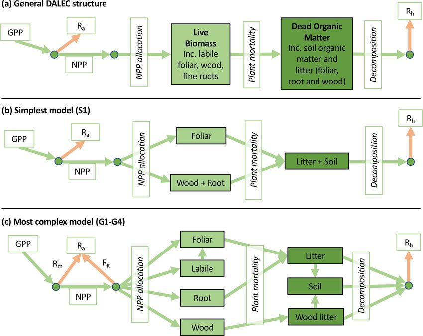
2728                              C. A. Famiglietti et al.: Optimal model complexity for terrestrial carbon cycle prediction

and Bonan, 2017; Bonan and Doney, 2018). Because the be-
havior of the terrestrial biosphere feeds back directly on the
rate of CO2 accumulation in the atmosphere, understanding
the most effective ways of reducing this model uncertainty is
crucial. Progress can benefit not only long-term predictions
of global change, but also near-term, regional-scale ecologi-
cal forecasts aimed at informing sustainable decision-making
(Dietze et al., 2018; Thomas et al., 2018; White et al., 2019)
and modeling studies focused on understanding the recent
past (Schwalm et al., 2020).
    While ecological models are becoming more and more de-
tailed, the extent to which predictive skill scales with model
complexity is not clear. The logic behind enhancing model
realism with increased complexity is intuitive: a highly sim-       Figure 1. Conceptual diagram of effective complexity in three-
                                                                    parameter space. A sphere (a) has three unique dimensions span-
plistic model may be structurally unable to capture key rela-
                                                                    ning the three axes of variability (analogous to a larger solution
tionships defining the system (it underfits), which would nat-      space for a given model). In the region defined by the same three
urally imply that greater detail is needed to improve model         axes, a disc (b) has only two unique dimensions (analogous to a
performance. However, excessively complex models have               smaller solution space, perhaps due to two parameters being highly
their own limitations. Because they often contain more pa-          correlated).
rameters than can be robustly determined with the available
data (e.g., Prentice et al., 2015; Shi et al., 2018; Feng, 2020),
they are prone to learning “noise” instead of true interac-         lution space. When locations or data constraints do not al-
tions (also called overfitting; Ginzburg and Jensen, 2004;          low certain model parameter values or modeled states, this
Hawkins, 2004; Keenan et al., 2013). Equifinality – the case        reduces the effective complexity of the remaining set of pos-
in which vastly different parameter sets can yield similar          sible solutions. That is, one can consider what we term the
model performance (Beven, 1993; Beven and Freer, 2001)              “effective complexity” of a model as a function of the ac-
– also becomes more likely as model complexity increases.           tual parameter combinations that are possible for that model,
This dichotomy between model complexity and model per-              or equivalently, the volume of space occupied by these pa-
formance is known in the statistics and machine learning            rameter combinations. Two models with the same number of
communities as the bias–variance tradeoff. According to this        parameters may have very different effective complexities,
theory, a model that balances the costs of under- and over-         for example, because correlations between parameters (e.g.,
fitting can minimize forecast error (Lever et al., 2016). It is     allocation fraction to foliage and turnover rate of foliage; Fox
therefore possible that other approaches to reducing carbon         et al., 2009) or the extent to which they are constrained (i.e.,
cycle model uncertainty (e.g., improving model parameteri-          many more states are possible in the absence of assimilated
zation) may be more effective than increasing structural real-      data than in the presence of it; Keenan et al., 2013), or when
ism in some circumstances, as also noted by Shiklomanov et          the assimilated data have high uncertainty, can influence the
al. (2020) and Wu et al. (2020a).                                   models’ effective degrees of freedom. As a simple analogy,
    Here, we explicitly map the relationship between model          consider the difference between a sphere and a disc in three-
complexity and predictive performance across a spectrum of          dimensional space (Fig. 1). Although both exist within the
model structures and parameterizations, hypothesizing that          space determined by three unconstrained parameters (axes),
an intermediate-complexity carbon cycle model can outper-           they are not identical because the volumes they occupy – and
form a low- or high-complexity one. Our approach can in-            the relationships between their parameters – are drastically
form ecological models that operate on a spectrum of scales,        different. The same can be true between models: one model’s
from localized at the level of individual stands to highly gen-     equations or assimilated observations may constrain the di-
eralizable across the global land surface. This study is par-       mensionality of its potential parameter space to “resemble” a
ticularly relevant for global ecological models, which often        disc, while that occupied by another, less constrained model
function as the land surface component of large-scale Earth         may look more like a sphere.
system models and have been employed in contexts that carry            Model–data fusion (MDF) systems (also known as data
significant policy relevance (e.g., Intergovernmental Panel on      assimilation systems) provide an effective way of isolating
Climate Change (IPCC) reports; Stocker et al., 2014). Here-         and evaluating different model structures by using obser-
after we refer to global ecological models as terrestrial bio-      vations to derive optimized model parameters with uncer-
sphere models, or TBMs.                                             tainty. An increasingly common tool for carbon cycle sci-
    We note a distinction between conceptualizing complex-          ence, MDF has been leveraged to provide insight into long-
ity as a straightforward count of a model’s parameters, equa-       term trends of carbon fluxes (e.g., Rayner et al., 2005), to rec-
tions, or processes, versus as an emergent property of its so-      oncile the roles of specific datasets in constraining paramet-

Biogeosciences, 18, 2727–2754, 2021                                                    https://doi.org/10.5194/bg-18-2727-2021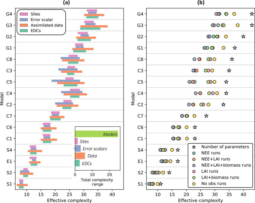
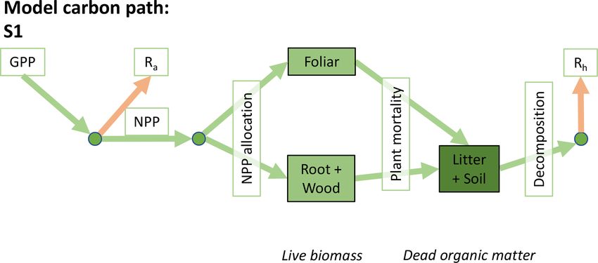
C. A. Famiglietti et al.: Optimal model complexity for terrestrial carbon cycle prediction                                   2729

ric uncertainty (e.g., Keenan et al., 2013), and more (Scholze     2     Methods
et al., 2017). Here we use an MDF system called the CAR-
bon DAta MOdel fraMework, or CARDAMOM (Bloom and                   2.1    Suite of carbon cycle models (DALEC variants)
Williams, 2015; Bloom et al., 2016), chosen because of its
high customizability. The structure of its underlying ecosys-      The Data Assimilation Linked Ecosystem Carbon (DALEC)
tem carbon model, DALEC (Williams et al., 2005; Bloom              model suite includes 16 related intermediate-complexity
and Williams, 2015), can be easily adjusted to become more         models of the terrestrial carbon cycle. Each model variant
simple or detailed (e.g., by changing the number of carbon         tracks the state and dynamics of both live and dead carbon
pools or by modifying the functional representations of cer-       pools, their interactions, and responses to meteorology and
tain carbon fluxes). Various combinations of observational         disturbance such as fire or biomass removals. From an initial
and functional constraints can also be tested in the assimila-     DALEC model (Williams et al., 2005), we produced alternate
tion process, along with different assumptions on the amount       structures that either aimed to reduce complexity by focusing
of error inherent to each assimilated dataset (the character-      on core variables/processes and removing others or aimed to
ization of which is an ongoing challenge for the modeling          increase complexity by including hypothesized missing car-
community; Keenan et al., 2011). Taken together, this flexi-       bon pools or improving on over-simplified processes.
bility allows for experimentation with the different levers that      Accordingly, the DALEC suite spans a range of model
control effective model complexity.                                structures (i.e., number of carbon pools, carbon pool connec-
   In this paper, we demonstrate the extent to which the pre-      tivity) and process representations (component sub-models
diction accuracy of two key carbon cycle variables can the-        of varying complexity) related to different simulations of
oretically scale with model complexity. Net ecosystem ex-          photosynthesis, plant respiration, decomposition, and water
change (NEE) and leaf area index (LAI) were chosen for the         cycle feedbacks. These representations are listed in Table 1
analysis because they represent integrated effects of different    and described in further detail in Appendix A. To facilitate
parts of the carbon cycle (NEE is the balance of photosyn-         disentanglement of the impacts of specific alternate process
thesis and ecosystem respiration fluxes, while LAI strongly        representations, the different sub-models can be related to a
controls canopy photosynthesis; Bonan, 1993). Additionally,        common baseline structure of the carbon cycle (Fig. 2a). Spe-
both are commonly measured and modeled. To explore the             cific variants of this general structure for the least and most
complexity–skill relationship, we developed 16 structurally        detailed models in this analysis are presented in Fig. 2b–
distinct carbon cycle models (i.e., variants of the DALEC          c, while additional diagrams for the remaining models are
model) spanning a range of complexity and calibrated them          shown in Appendix B (Figs. B1–B7). Across models, car-
using the CARDAMOM framework. Several recent studies               bon enters the system via gross primary productivity (GPP),
have demonstrated the utility of CARDAMOM for under-               which is allocated to autotrophic respiration (Ra ) and non-
standing multiple aspects of the carbon cycle (e.g., López-        canopy live tissues based on fixed fractions. Canopy growth
Blanco et al., 2019; Konings et al., 2019; Yin et al., 2020;       and mortality is determined by a phenology sub-model which
Bloom et al., 2020; Quetin et al., 2020), lending confidence       is sensitive to day of year (sub-model scheme CDEA), envi-
for its use here. We calibrated each DALEC variant within          ronmental factors (GSI), or a combination of environmen-
CARDAMOM under 42 different data scenarios (i.e., com-             tal factors and estimated net canopy carbon export (NCCE).
binations of data constraints and assumptions about observa-       Mortality of wood and fine roots follows continuous turnover
tional error) representing different degrees of certainty with     based on first-order kinetics. Decomposition of dead organic
which parameters are determined. Each model was calibrated         matter and associated heterotrophic respiration (Rh ) follows
and validated at six globally distributed eddy covariance sites    first-order kinetics with an exponential temperature sensitiv-
covering a range of biomes and vegetation types, with data         ity (and, in models C2–C5, a linear soil moisture sensitivity).
collected over multiple years. To quantify complexity, we
computed the effective complexity of each model calibra-           2.2    Site selection
tion using a principal component analysis (PCA) that reduced
the parameter space to its primary axes of variance. Forecast      COMPLEX uses information from six globally distributed
skill was determined using an overlap metric that takes ac-        eddy covariance sites participating in FLUXNET (Pastorello
count of uncertainty both in the model forecast and the val-       et al., 2020) (Table 2). Our site selection procedure aimed
idation data. Though the range of complexity we evaluated          to maximize biogeographical spread and diversity of natural
here is lower than that populated by large-scale TBMs, this        ecosystems while fulfilling specific data requirements. These
experiment reveals universal modeling elements that control        constraints collectively yielded a series of site selection cri-
performance. Specifically, here our COMPLexity EXperi-             teria that are described in detail in Appendix C. As an exam-
ment (COMPLEX) aims to answer the following questions.             ple, the sites must not be dominated by the C4 photosynthetic
(a) What controls a given model run’s effective complexity?        pathway, nor arable agriculture nor intensively grazed grass-
(b) Under what conditions does increasing model complexity         land. Additionally, we required that the range of time series
improve forecast skill?                                            observations to be used for model calibration and validation

https://doi.org/10.5194/bg-18-2727-2021                                                    Biogeosciences, 18, 2727–2754, 2021
C. A. Famiglietti et al.: Optimal model complexity for terrestrial carbon cycle prediction
https://doi.org/10.5194/bg-18-2727-2021
Table 1. Summary of the DALEC sub-model combinations assessed in COMPLEX. For a detailed description see the Supplement. ID is model identifier. CDEA: Combined Deciduous
Evergreen Analytical model; CDEA+: CDEA with variable labile release fraction; GSI: growing season index; NCCE: net canopy carbon export; ACM: aggregated canopy model;
T : temperature; M: soil moisture; CUE: carbon use efficiency. fNPP : GPP indicates a fixed fractional allocation of gross primary production (GPP) to foliage net primary production
(NPP). DOM is dead organic matter. Models are grouped according to common characteristics, as follows: C models all share the Combined Deciduous Evergreen Analytical (CDEA
or CDEA+) phenology sub-model; G models use the growing season index (GSI) phenology sub-model; E models use the evergreen (constant allocation) phenology sub-model; and S
models are simple, reduced-complexity variants of other models.
ID Canopy Method of Water Rh CUE Number of DOM Live
phenology computing GPP cycle parameters pools pools
C1 CDEA ACM v1 No T Ra : GPP 23 2 4
C2 CDEA+ ACM v1 Yes T +M Ra : GPP 33 2 4
C3∗ CDEA+ ACM v1 Yes T +M Ra : GPP 35 2 4
C4a CDEA+ ACM v1 Yes T +M Ra : GPP 34 2 4
C5 CDEA+ Analytical Ball–Berry Yes T +M Ra : GPP 34 2 4
C6 CDEA ACM v2 No T Ra : GPP 23 2 4
C7 CDEA ACM v2 Yes T Ra : GPP 27 2 4
C8b CDEA ACM v1 Yes T Ra : GPP 36 2 4
E1 fNPP : GPP ACM v1 No T Ra : GPP 17 3 3
G1 GSI ACM v2 No T Rm : GPP + Rg : NPP 37 3 4
G2 GSI ACM v2 Yes T Rm : GPP + Rg : NPP 40 3 4
G3 GSI + NCCE ACM v2 No T Rm Leaf(T ) + Rm Wood : GPP + Rm Root : GPP + Rg : NPP 43 3 4
G4 GSI + NCCE ACM v2 Yes T Rm Leaf(T ) + Rm Wood : GPP + Rm Root : GPP + Rg : NPP 43 3 4
S1 fNPP : GPP ACM v1 No T Ra : GPP 11 1 2
Biogeosciences, 18, 2727–2754, 2021
S2 CDEA ACM v1 No T Ra : GPP 14 1 3
S4 CDEA ACM v1 No T Ra : GPP 17 3 2
∗ Includes cold weather GPP limitation. a Includes surface runoff parameterization (assumes constant runoff to infiltration ratio at surface). b Includes two water storage pools (plant-available and
plant-unavailable water).
2730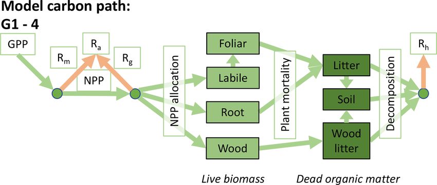
C. A. Famiglietti et al.: Optimal model complexity for terrestrial carbon cycle prediction                                              2731

Figure 2. Overview of the carbon pools (filled boxes) and fluxes (arrows, with names in open boxes) represented in the DALEC model suite.
(a) Broad structure of the DALEC model maintained across all variants in the suite; (b) carbon cycle structure of the simplest model; (c) car-
bon cycle structure of the most detailed model.

spanned at least a decade. Data collated at each site are de-            CARDAMOM is the imposed constraint that litter turnover
scribed below (see Sect. 2.3).                                           times are faster than soil organic matter turnover times (e.g.,
                                                                         Gaudinski et al., 2000). In this analysis, each model includes
2.3   Model–data fusion                                                  some or all of the EDCs documented in Bloom et al. (2016).
                                                                            The likelihood p (O|y) is derived as a function of
We used the CARDAMOM model–data fusion system                            the mismatch between observations O and the model
(Bloom and Williams, 2015; Bloom et al., 2016) to param-                 realization M corresponding       to y, such that p (O|y) ∝
                                                                                                 2
eterize the DALEC model suite with available observations                         1 PN

                                                                                           On −Mn
of the carbon cycle. Specifically, we employed Bayesian in-              exp − 2 n=1         σn        , where σn is the error for the
ference to retrieve time-invariant, site-specific, optimized pa-         nth observation. This formulation requires no assumptions
rameters and initial conditions for a given DALEC model                  on the normality of prior or posterior parameter distri-
(y) as informed by observations (O), where p(y|O) ∝ p(y)·                butions and is robust to missing data. In our analysis,
p(O|y). Here, p(y|O) is the posterior parameter probability              monthly-averaged eddy covariance NEE measurements from
distribution, p(y) is the prior parameter probability distribu-          FLUXNET, monthly-averaged leaf area index (LAI) esti-
tion, and p(O|y) is proportional to the likelihood of param-             mates from the Copernicus Global Land Service (Verger
eters y given observations O.                                            et al., 2014; Fuster et al., 2020), and in situ wood stock
   For each model, p(y) is derived as the product of (i) the             surveys were made available for ingestion into the model
prior probability density functions for each model parame-               (see Appendix C). NEE uncertainty was assumed to be
ter and (ii) ecological and dynamical constraints (EDCs, i.e.,           0.58 gC m−2 d−1 based on estimates of random errors in
functional constraints). EDCs are simple mathematical func-              eddy covariance measurements from Hill et al. (2012). A
tions that impose conditions on inter-relationships between              time-varying uncertainty estimate was included with the
model parameters based on known ecological theory. They                  Copernicus LAI product, and site-specific, locally derived
are used to inform parameter prior information with broader              biomass uncertainties were provided by the site PI or drawn
ecological knowledge and tend to reduce bias and equifinal-              from relevant publications when necessary. Model drivers in-
ity (Bloom and Williams, 2015). One example of an EDC in

https://doi.org/10.5194/bg-18-2727-2021                                                           Biogeosciences, 18, 2727–2754, 2021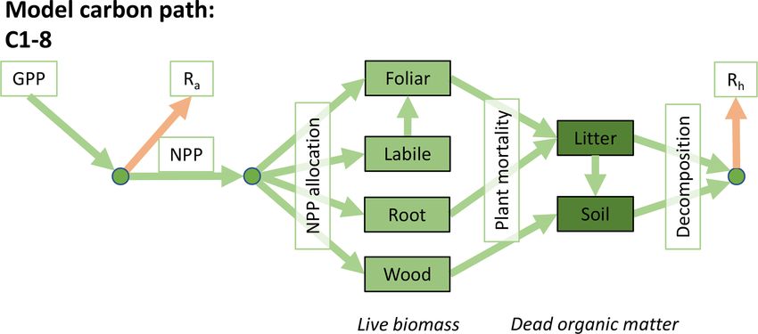
2732 C. A. Famiglietti et al.: Optimal model complexity for terrestrial carbon cycle prediction
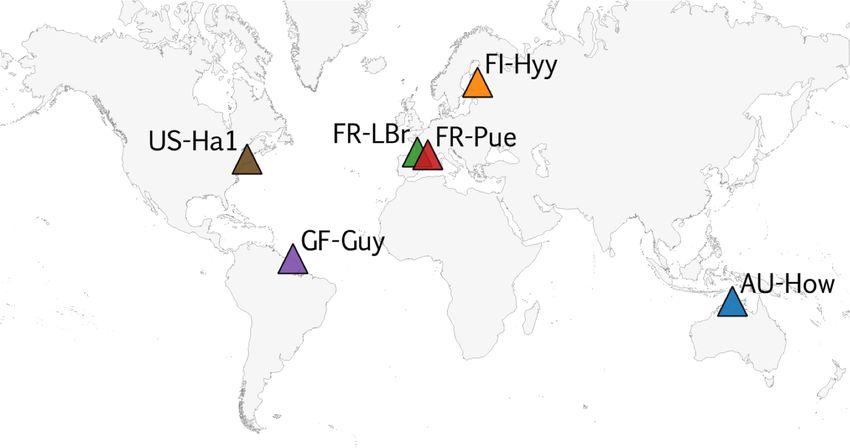
Table 2. Summary of sites, showing their location, FLUXNET code, observational time period, mean climate information, and ecosystem
type. Latitude is given in −90/90 and longitude is −180/180. Ecosystem type is denoted using the International Geosphere-Biosphere
Programme (IGBP) classification. DBF: deciduous broadleaf forest; EBF: evergreen broadleaf forest; ENF: evergreen needleleaf forest;
WSA: woody savanna.
Site name Site code Reference Latitude Longitude IGBP Data Mean Mean
record annual annual
temp. precip.
[◦ C] [mm yr−1 ]
Howard Springs AU-How Beringer et al. (2007) −12.4943 131.1523 WSA 2001–2014 27.0 1449
Hyytiälä FI-Hyy Suni et al. (2003) 61.84741 24.29477 ENF 1999–2014 3.8 709
Le Bray FR-LBr Berbigier et al. (2001) 44.71711 −0.7693 ENF 1998–2008 13.6 900
Puéchabon FR-Pue Rambal et al. (2004) 43.7413 3.5957 EBF 2000–2014 13.5 883
Guyaflux GF-Guy Aguilos et al. (2018) 5.27877 −52.92486 EBF 2004–2018 25.7 3041
Harvard Forest US-Ha1 Munger and Wofsy (2020a, b) 42.5378 −72.1715 DBF 1998–2012 6.2 1071
cluded monthly average site meteorology (air temperature, Table 3. Model specifications varied in the factorial experiment.
shortwave radiation, atmospheric CO2 concentration, vapor Each of the 16 model versions was run with every combination of
pressure deficit, precipitation, and wind speed). Here models scenarios across each variable. Note that observational error scalars
were run at the monthly time step. were not applied when no data were assimilated into the model.
To sample the distribution p(y|O) (namely the prod-
uct of p (O|y) and p (y)), we used an adaptive proposal Variable Scenarios
Metropolis–Hastings Markov chain Monte Carlo (MCMC) Site AU-How
approach (Haario et al., 2001). We performed 108 iterations FI-Hyy
for each of four chains, which were checked for conver- FR-LBr
gence using the Gelman–Rubin criterion (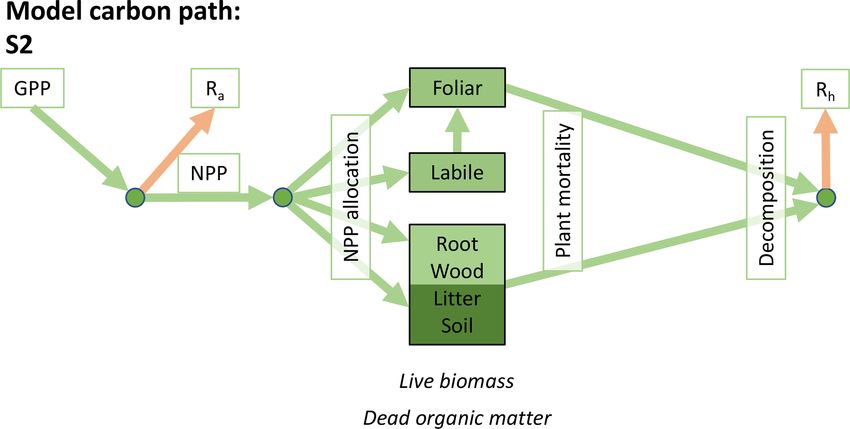
C. A. Famiglietti et al.: Optimal model complexity for terrestrial carbon cycle prediction 2733
time series based only on prior parameter distributions are sions necessary to explain the most variability in the pos-
presented in Fig. S1. terior parameter space of each model analysis. Specifically,
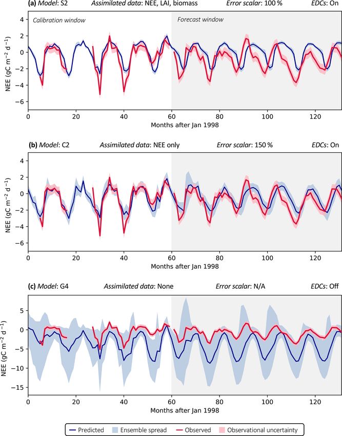
Accounting for prediction uncertainty – as well as data un- we defined effective complexity as the number of principal
certainty (red shading) – is a key goal of our model skill components for which 95 % of variance in the posterior pa-
evaluation approach. Forecast skill for each model run was rameter space was explained. Note that in our experiment, a
computed by comparing predictions and observations drawn given DALEC model variant has a distribution of effective
strictly from the forecast period, using the histogram inter- complexities corresponding to the different specifications for
section algorithm (see Sect. 2.5.1). The complexity of each each run (i.e., data scenario, site; Table 3).
run was quantified based on its effective complexity (see
Sect. 2.5.2).
2.5 Analysis 3 Results
2.5.1 Skill metric 3.1 Behavior of effective complexity metric
We chose the histogram intersection as a skill metric because Effective complexity – defined as the number of principal
it captures accuracy along with both prediction uncertainty components for which 95 % of the variance in the posterior
(i.e., the ensemble spread for a given model output) and ob- parameter space is explained (see Sect. 2.5.2) – is primarily
servational uncertainty (i.e., the mean value and error for a determined by model structure (Fig. 4a, inset). Specifically,
given observation). This approach contrasts with more famil- over all runs included in the experiment, effective complex-
iar metrics such as the coefficient of determination (R 2 ) or ity varies far more between different models than between
root-mean-square error (RMSE), which do not account for the other tested factors (assimilated data, observational er-
uncertainties surrounding individual data points or predic- ror scalar, site, and EDC presence or absence). This link
tions. to model structure provides insight into the metric’s inter-
The histogram intersection is a simple algorithm that cal- pretability and justifies its use as a measure of model com-
culates the similarity of two discretized distributions p and plexity.
q and is commonly used in the machine learning commu- While predominantly determined by the choice of model,
nity (e.g., for image classification; Jia et al., 2006; Maji et effective complexity also varies according to the degree to
al., 2008). Specifically,
P the histogram intersection of p and which parameters are constrained (Fig. 4a). It therefore cap-
q is computed as ni=1 min (pi , qi ), where n is the number tures the inter-relationship between model structure and pa-
of bins in the two histograms (here, n was set to 50). In our rameterization. Within a given model structure, each of the
case, p was the histogram of predicted NEE or LAI ensem- experimentally varied factors yields a range of distinct com-
bles for a given time step, and q was a discretized Gaussian plexities that follows a predictable pattern: effective com-
distribution with mean and standard deviation equivalent to plexity is higher for runs with weaker constraints on pa-
the observed NEE or LAI value P and its error, respectively. rameters than it is for runs with stronger constraints on pa-
We normalize the metric by ni=1 pi so that it is bounded be- rameters. This is easily interpretable in the case of assimi-
tween 0 (no overlap) and 1 (identical distributions). Because lated data, which is the dominant within-model control on
histograms p and q correspond to individual months in the effective complexity (Fig. 4b). Runs for which no observa-
forecast period, the metric used for analysis was the average tions are ingested into the model have consistently higher
histogram intersection over all such months. effective complexities than runs for which NEE, LAI, and
We note that results for NEE predictions are presented in biomass observations are all ingested (compare yellow and
the main figures of this paper, while those for LAI predictions purple circles in Fig. 4b), since the observational constraints
are included in the supporting information. reduce the possible model solution space. Similar behavior
is also observed across the different error scalars tested in
2.5.2 Complexity metric the experiment (larger observational error assumptions cor-
respond to higher effective complexities (Fig. S2)) and be-
The effective complexity of each model run links model tween the presence versus absence of EDCs (the absence
structure (i.e., process representation) and number of param- of non-observational realism constraints yields higher effec-
eters to the information content of assimilated data. It was tive complexities (Fig. S3)). Conceptually, this pattern can
computed using a principal component analysis (PCA) on the be understood in the following way. Parameters in a given
posterior parameter space. When applied to CARDAMOM model’s high-complexity runs were sampled from wider pos-
output, the PCA reduces the posterior parameter space (n terior distributions (due to weak or absent constraints) than
ensembles of m parameters) to a set of at most m uncorre- in its low-complexity runs. This implies greater variance be-
lated variables that successively maximize variance. As such, tween parameter sets selected in high-complexity runs – and
this approach finds the smallest number of unique dimen- thus more distinct dimensions of variability in the posterior
https://doi.org/10.5194/bg-18-2727-2021 Biogeosciences, 18, 2727–2754, 2021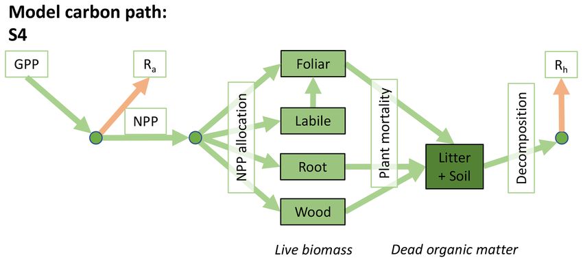
2734                                C. A. Famiglietti et al.: Optimal model complexity for terrestrial carbon cycle prediction

Figure 3. Example model runs (title of each subplot) at the FR-LBr site. The calibration window – the first 5 years of the record – is
shown in white, and the forecast window is shaded gray. The ensemble spread (blue shading) encapsulates the 5th–95th percentiles of runs.
(a) Forecast skill = 0.15; effective complexity = 7; (b) forecast skill = 0.44; effective complexity = 24; (c) forecast skill = 0.22; effective
complexity = 39.

parameter space – than in low-complexity runs for the same                (Fig. S4a). Runs on both extremes of the complexity axis per-
model.                                                                    form poorly, due to overfitting in the low-complexity case
                                                                          (parameters are over-determined, leading to accurate predic-
3.2    Relationship between effective complexity and skill                tions in the training period but poor ones in forecast) and un-
                                                                          derfitting in the high-complexity case (parameters are under-
Across all runs performed in the experiment, the hypothesis               determined, yielding poor predictions in both training and
that an intermediate-complexity carbon cycle model can out-               forecast). Figure 3a and 3c demonstrate this contrasting be-
perform a low- or high-complexity model is confirmed, both                havior at the FR-LBr site.
when NEE is predicted (Fig. 5a) and when LAI is predicted

Biogeosciences, 18, 2727–2754, 2021                                                           https://doi.org/10.5194/bg-18-2727-2021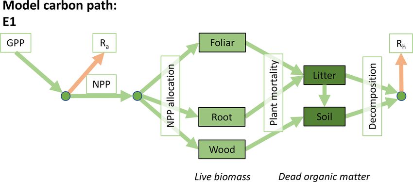
C. A. Famiglietti et al.: Optimal model complexity for terrestrial carbon cycle prediction                                                2735

Figure 4. Influence of the experimentally varied factors on effective complexity. (a) Range of effective complexity attributable to sites, error
scalars, assimilated data, and EDCs for each model (row). Inset: range of attributed effective complexity across all model runs. (b) Average
effect of assimilated data combination on effective complexity for each model. Colored circles are means of corresponding runs. Models are
ordered from fewest (S1) to greatest (G4) number of parameters. See Table 1 for definition of model IDs.

   When runs for which no data were assimilated – that is,                adequately informed by data). Importantly, larger observa-
runs with the least informed parameters – are withheld from               tional uncertainty assumptions reduce the effectiveness of as-
the analysis, increasing complexity no longer degrades skill              similated data at constraining parameters in high-complexity
(Fig. 5b). More specifically, the relationship between ef-                models. The monotonically increasing relationship between
fective complexity and skill increases monotonically when                 complexity and skill is strongest when observational error is
all runs have some baseline constraint on parameters. This                assumed to be relatively small (Fig. S6).
result also holds regardless of which variable is predicted                  Assimilated data determine the shape of the overall
(Fig. S4b) as well as when the number of runs within each                 complexity–skill relationship in COMPLEX. Not only does
complexity bin is standardized via bootstrapping (Fig. S5).               the presence of any assimilated observations control the re-
The decline in performance attributable to the most ex-                   sponse of skill to increasing complexity, but the specific
treme effective complexity scenarios is also preserved across             choice of assimilated observations also matters. In particu-
RMSE and R 2 metrics (not shown; further comparison be-                   lar, assimilating monthly NEE observations improves both
tween different metrics is beyond the scope of this paper).               NEE (Fig. 6a–c) and LAI predictions (Fig. S7a–c) by com-
This finding implies that increasing complexity by introduc-              plex models over simple models: note the positive/increasing
ing suitable data-constrained parameters can improve perfor-              trends between complexity and skill in these cases. However,
mance, but that doing so by adding unconstrained dimen-                   such improvements in predictive performance are not consis-
sions can degrade it. That is, the processes and parameters               tently observed across the complexity axis when other data,
introduced in the most detailed models (such as G1–G4) can                but not NEE, are ingested. The ingestion of LAI data and
lead to improvements in predictive skill over simpler mod-                biomass estimates yields a small positive trend (Fig. 6d) –
els only when they are sufficiently well-characterized (i.e.,             although this relationship is clearly weaker than when NEE

https://doi.org/10.5194/bg-18-2727-2021                                                             Biogeosciences, 18, 2727–2754, 2021
2736                              C. A. Famiglietti et al.: Optimal model complexity for terrestrial carbon cycle prediction

Figure 5. Relationship between effective complexity and NEE forecast skill for (a) all model runs in the experiment and (b) the subset of
runs in panel (a) for which data were assimilated. Dark gray shading spans the 25th to 75th percentiles of runs; light gray shading spans
the 5th to 95th percentiles; blue points are medians of effective complexity bins. Average forecast skill is computed using the histogram
intersection metric.

is also assimilated (Fig. 6a) – and simple models informed             sites included in our analysis demonstrate additional unique
only by LAI perform just as well as complex models when                dynamics. GF-Guy is the only site for which the performance
predicting NEE. Indeed, these runs show a constant skill               of the most complex models appears to slightly degrade, even
level across the complexity axis (Fig. 6e). When predict-              when all observations including NEE are assimilated, and
ing LAI, though, complex models outperform simple models               no threshold is apparent at AU-How. Overall, the site anal-
with only the assimilation of LAI (Fig. S7e). All such com-            ysis demonstrates the large variability in model performance
binations contrast with the case in which no data are assimi-          across space, including between sites sharing biome classifi-
lated: forecast skill for those runs declines with complexity,         cations (e.g., FI-Hyy and FR-LBr) or broadly similar climate
regardless of target variable (Figs. 6f, S7f).                         types (e.g., GF-Guy and AU-How).
   Recall that the magnitude of skill – the degree of overlap
between model predictions and observations (see Sect. 2.5.1)
– reflects the ability of the model to capture the data along          4     Discussion
with its uncertainty. Particularly in scenarios corresponding
to low effective complexities, models tend to overfit when             4.1    Effective complexity and the inter-relationship
NEE is assimilated (as demonstrated in Fig. 3a). Overfitting                  between model structure and parameterization
is a key factor causing the discrepancy in performance be-
tween low-complexity runs that do (e.g., Fig. 6c) and do not           We defined a concept of effective complexity that is linked to
assimilate NEE (e.g., Fig. 6e).                                        model structure and number of parameters as well as to the
   Regardless of which data are assimilated, site-specific             information content of calibration data (Fig. 4). This met-
characteristics also introduce additional variability into the         ric can inform future studies seeking to investigate the role
form of the relationship between effective complexity and              of model complexity by providing a simple and comparable
skill (Fig. 7). To better understand and isolate site-specific         quantification of parameter posteriors. Conventional com-
dynamics, here we only interpret runs for which at least one           plexity measures (e.g., counts of observable model attributes)
data type is assimilated. Most sites show high-complexity              can serve as reasonable approximations of the more nuanced
performance optima, consistent with Fig. 5b. However, sev-             definition specific to ensemble methods that we present here.
eral are characterized by a threshold effect for which perfor-         Still, effective complexity is rarely identical to the number of
mance increases significantly once a certain effective com-            model parameters: it is generally lower. Correlations between
plexity is attained and remains stagnant thereafter (e.g., a           model parameters can and do occur whether the model is
low-complexity threshold around 10 for FI-Hyy and FR-                  poorly or well-constrained (Keenan et al., 2013) and whether
Pue). This “diminishing returns” effect suggests that the per-         it is simple or complex, implying that all carbon cycle mod-
formance benefit of added structural detail has the potential          els have “constrainable” dimensions. Importantly, though,
to stabilize for all but the simplest models. The two tropical         none of the high-parameter models in our experiment have
                                                                       so much redundancy that their average effective complexity

Biogeosciences, 18, 2727–2754, 2021                                                       https://doi.org/10.5194/bg-18-2727-2021
C. A. Famiglietti et al.: Optimal model complexity for terrestrial carbon cycle prediction 2737
Figure 6. Complexity–skill relationship for NEE predictions, split by combination of assimilated data (title of each subplot). Average forecast
skill is computed using the histogram intersection metric. Ordering of subplots reflects the strongest (a) to weakest (f) data constraint.
across runs is equivalent to that of any low-parameter model ence gains in skill with increased complexity than those that
(Fig. 4). Whether this is also true for large-scale TBMs re- cannot. This result is consistent with the prominent role of
mains an open question. NEE observations in reducing model projection uncertainty
Overall, the behavior of the effective complexity met- identified by Keenan et al. (2013). The effects of LAI and
ric highlights that the best-performing analyses (i.e., runs biomass observations in COMPLEX are somewhat more nu-
with the highest forecast skill) in the COMPLEX maximize anced. All models in the DALEC suite are able to extract in-
model structural breadth and minimize parametric uncer- formation from the LAI data and produce reasonably skilled
tainty. Models built with high numbers of processes but with- NEE predictions (Fig. 6e), though such data do not improve
out effective parameter constraints (i.e., runs that maximize the skill of complex models over simple ones. The ingestion
structural breadth but do not attempt to minimize paramet- of LAI data most directly constrains specific features relat-
ric uncertainty) are not sufficient to optimize performance ing to growth or carbon allocation, potentially informing the
(Fig. 5). Additionally, models of the carbon cycle can overfit seasonality of NEE. Finally, the impacts of biomass obser-
if they are calibrated in too narrow a subset of conditions and vations on forecast skill were relatively muted in our exper-
underfit if they are improperly parameterized and therefore iments. Given that biomass data are particularly useful for
biased, as shown in Fig. 3. informing the carbon cycling of slow pools (Williams et al.,
2005), the relatively short calibration (5 years) and forecast
4.2 Influence of data constraints and site on periods (≥ 5 years) tested here, along with the temporal spar-
complexity–skill relationship sity of these data in COMPLEX (i.e., a few measurements per
site instead of continuous time series for LAI or NEE), may
The main factors controlling the observed complexity–skill have obscured their utility.
relationship are (a) whether, and which, data are assimilated Several recent TBM efforts have sought to enable the as-
into the model and (b) the geographical location at which similation of eddy covariance or remote sensing observations
the analysis is undertaken. One way to interpret the role of (e.g., Bacour et al., 2015; Raoult et al., 2016; Schürmann et
data in the relationship is explicit: models with the ability al., 2016; Peylin et al., 2016; MacBean et al., 2018; Norton et
to assimilate monthly observations of NEE, which uniquely al., 2019) as well as measurements of functional traits (e.g.,
represent the integrated behavior of terrestrial carbon cy- LeBauer et al., 2013). Our results underscore the value of
cling and its internal dynamics, are more likely to experi- such efforts to reduce parameter uncertainty, despite the fact
https://doi.org/10.5194/bg-18-2727-2021 Biogeosciences, 18, 2727–2754, 20212738 C. A. Famiglietti et al.: Optimal model complexity for terrestrial carbon cycle prediction Figure 7. Complexity–skill relationship for NEE predictions, split by site (title of each subplot). Only runs for which data were assimilated are plotted. Average forecast skill is computed using the histogram intersection metric. that the computational costs associated with data assimilation model performance accrued by the addition of a given pro- are relatively high (e.g., MacBean et al., 2016). Increased use cess should not be expected to affect all locations uniformly, of emulators may help reduce this computational cost (Fer et even when site-specific parameter uncertainty is minimized al., 2018). through calibration or optimization. Models not tuned locally Given the demonstrated value of data constraints and the likely smooth this spatial variability in predictability drasti- specification of their uncertainty (Fig. S6), the need to char- cally (van Bodegom et al., 2012; Berzaghi et al., 2020), and acterize and quantify this uncertainty (Keenan et al., 2011) thus model development and calibration must include loca- remains particularly critical for model–data fusion studies. tions spanning a wide range of vegetation, climate, soil char- In this analysis, NEE uncertainty was assumed to remain acteristics, and disturbance histories. constant both in time (i.e., for all observations regardless of season or year) and in space (i.e., across sites), which likely 4.3 Recommendations for selecting appropriate model over-generalizes the specifications of individual sensors and complexity the possibility of systematic or increasing biases. These as- sumptions become even more important to account for when Overall, our results suggest that the benefits of increased assimilating global datasets, for which retrieval accuracy can model complexity (e.g., gains in skill attributable to the in- vary across land cover types or with atmospheric conditions troduction of specific processes or to additional detail ap- such as clouds or snow (e.g., Fang et al., 2013). One bene- plied to existing mechanisms) are attainable only when pa- fit of the Copernicus LAI product used here is its explicit, rameters are sufficiently well characterized. Here, this ben- spatially variable quantification of uncertainty, which is still efit is achieved when high complexity is balanced by data- relatively rare for remote sensing datasets. Though the ro- assisted parameter optimization (in particular, when NEE ob- bustness of these uncertainties has been challenged with in- servations are assimilated). More broadly, the relationship dependent observations in some locations (e.g., Zhao et al., between complexity and skill is dynamic and extends beyond 2020), this approach represents a level of detail well-suited model structural choices. As a result, it is difficult to quan- to the coupling of data to large-scale or global models. tify whether model parameters corresponding to any spe- The observed variability in the complexity–skill relation- cific model implementation – including outside the DALEC ship across sites (Fig. 7) suggests that predictability itself is suite – are adequately informed such that increased model spatially heterogeneous. Further, it implies that the benefit to complexity is beneficial to performance. To assist in this en- Biogeosciences, 18, 2727–2754, 2021 https://doi.org/10.5194/bg-18-2727-2021
C. A. Famiglietti et al.: Optimal model complexity for terrestrial carbon cycle prediction                                   2739

deavor, we present the following recommendations for model        to the omission rather than inclusion of various processes,
development and evaluation.                                       suggesting a tradeoff between complexity and skill similar
                                                                  to that observed here. This conclusion calls into question the
 1. Assimilate well-characterized, repeat-observation             conventional paradigm that greater complexity significantly
    datasets to constrain model parameters at the scale of        and consistently improves skill across current TBMs.
    model application.                                               Earth observation (EO) is one key approach that can
 2. Use long time series to undertake independent forecast        provide the high-spatial- and high-temporal-resolution data
    evaluation studies, and factor observational uncertainty      on carbon cycling needed for more localized calibrations
    into model evaluation (e.g., using overlap metrics).          (Exbrayat et al., 2019). In COMPLEX, we used Coperni-
                                                                  cus LAI data, though there are also opportunities to in-
 3. Test whether model updates that add complexity lead to        gest biomass maps from space lidar or radar, estimates
    forecast improvements (not only calibration improve-          of photosynthesis from solar-induced fluorescence (SIF),
    ments), and test for possible model simplification im-        and satellite-based atmospheric inversions of regional NEE,
    provements also.                                              among others, in future studies. If supplied with appropriate
                                                                  error estimates, these datasets can over time provide pow-
 4. Seek to calibrate or optimize model parameters even           erful constraints for high-resolution carbon cycle analyses
    when data assimilation is not possible (e.g., using           with TBMs or DALEC-like models. A key research goal is to
    optimality-based approaches; Walker et al., 2017; Jiang       determine the appropriate model complexity for maximizing
    et al., 2020).                                                the information content of these EO data for robust forecasts
  Finally, while beyond the scope of this study, future work      and analyses.
will investigate the linkage between specific processes or           Alternative methodologies for deriving ecosystem param-
process representations (e.g., the inclusion or exclusion of      eters outside the realm of PFTs are also becoming increas-
water cycling) and predictive performance to better parse         ingly common (van Bodegom et al., 2012; Bloom et al.,
ecological controls on the complexity–skill relationship.         2016; Exbrayat et al., 2018; Berzaghi et al., 2020; Fisher
                                                                  and Koven, 2020) and may represent a way forward in ad-
4.4   Transferability to large-scale models (TBMs)                dressing the tradeoff between structural and parametric un-
                                                                  certainty. Recent work has focused on upscaling in situ trait
This analysis tested a spectrum of structurally distinct rep-     data (e.g., from the TRY database; Kattge et al., 2020) to
resentations of the carbon cycle based on the intermediate-       yield spatially variable maps of key ecosystem parameters,
complexity ecosystem model DALEC, which allowed for               using modeled relationships with climate or canopy proper-
coupling with the CARDAMOM model–data fusion system               ties (often referred to as environmental filtering relationships,
in a computationally tractable manner. Because our findings       since the environment “filters” the possible distribution of pa-
are not explicitly linked to the roles of specific processes or   rameters at a given location; e.g., Verheijen et al., 2013; van
model features, however, their implications extend beyond         Bodegom et al., 2014; Butler et al., 2017), leaf economics
the use of DALEC-like models to a wide variety of ecologi-        (Sakschewski et al., 2015), or optimality theory (e.g., Smith
cal models, including TBMs.                                       et al., 2019). Other studies have investigated how TBM pa-
   Traditional (based on plant functional type, or PFT) pa-       rameters optimized at eddy covariance sites covary with cli-
rameter determination in TBMs is far from random. It is           mate (e.g., Peaucelle et al., 2019; Wu et al., 2020b). These
informed by data – for example, by hypotheses or gener-           efforts are not without their challenges, however. The spatial
alizations derived from prior literature (e.g., Oleson et al.,    coverage of in situ trait data as well as eddy covariance sites
2010; Lawrence et al., 2011) or by model calibration at spe-      is sparse relative to the large diversity of ecosystem behav-
cific locations (e.g., Williams et al., 1997) – and therefore     ior (Schimel et al., 2015), and such datasets also comprise a
endowed with ecological knowledge. Accordingly, TBM pa-           non-representative sample of species and disturbance histo-
rameters are likely more informed than the least constrained      ries (Sandel et al., 2015). These biases may limit the repre-
parameters retrieved in our analysis, which were freely sam-      sentativeness of the modeled relationships. Taking a differ-
pled from wide uniform distributions and caused the high-         ent approach, a small subset of models has also been devel-
complexity decline in performance (Fig. 5). However, while        oped to operate altogether independently from the paradigm
this may be true locally, the common assumption on unifor-        of PFTs (e.g., using trait-based approaches; Scheiter et al.,
mity of parameters within PFTs casts doubt on their precision     2013; Pavlick et al., 2013; Fyllas et al., 2014). Our results
across the regional or global scales at which TBMs typically      imply that these and future developments to improve the flex-
make predictions (van Bodegom et al., 2012). Indeed, using        ibility of model parameters will play critical roles in enabling
a suite of global TBMs participating in the Multi-scale Syn-      the trend of increasing model complexity and may be a more
thesis and Terrestrial Model Intercomparison Project (MsT-        fruitful avenue towards reducing the uncertainty of TBM pre-
MIP; Huntzinger et al., 2013), Schwalm et al. (2019) showed       diction than model structural changes and additions.
that increases in model performance were more often linked

https://doi.org/10.5194/bg-18-2727-2021                                                  Biogeosciences, 18, 2727–2754, 2021
2740 C. A. Famiglietti et al.: Optimal model complexity for terrestrial carbon cycle prediction 5 Conclusions Our approach to understanding the relationship between model complexity and model predictive performance is novel in its focus on sampling the spectrum of possible parameter uncertainty states for a variety of model structures and cal- ibration data. Taken together, lessons learned from the be- havior of the effective complexity metric as well as the data and site effects discussed here represent a comprehensive pattern: improving the robustness of parameter calibration is a prerequisite for effectively increasing structural com- plexity. Specifically, we found that increasing model com- plexity actively degrades predictive skill in the most extreme cases of parameter uncertainty. Assimilating data – particu- larly monthly observations of net ecosystem exchange – con- siderably improve the performance of complex models rela- tive to simple models, though the magnitude and persistence of this improvement vary across space. Overall, the growing focus on understanding and reducing parametric uncertain- ties within large-scale models (such as via direct data assim- ilation, the development and implementation of alternatives to PFTs, and parameter sensitivity analyses; e.g., Fisher et al., 2019, and more) is both a necessary direction and a sig- nificant opportunity for improving the predictability of the terrestrial biosphere. Our conclusion for model construction and usage matches those from other scientific fields, as stated by Albert Einstein: “to make the irreducible basic elements as simple and as few as possible without having to surrender the adequate representation of a single datum of experience” (Caprice, 2013). Biogeosciences, 18, 2727–2754, 2021 https://doi.org/10.5194/bg-18-2727-2021
C. A. Famiglietti et al.: Optimal model complexity for terrestrial carbon cycle prediction                                  2741

Appendix A: DALEC model descriptions                             hereafter known as ACM2 (Smallman and Williams, 2019).
                                                                 ACM2 builds on the ACM1 outline creating a model of
The Data Assimilation Linked Ecosystem Carbon (DALEC)            ecosystem water cycling to facilitate the implementation of a
model suite includes a range of related intermediate-            mechanistic stomatal conductance model linking the canopy
complexity models of the terrestrial carbon cycle. Each          to soil water via fine roots. ACM2 also optimizes the stomatal
model version is comprised of sub-models related to different    intrinsic water use efficiency (for details see Williams et al.,
simulations of photosynthesis, plant and heterotrophic res-      1996; Bonan et al., 2014). ACM2 simulates shortwave and
piration, canopy phenology, stomatal conductance, and the        longwave isothermal radiation balances, canopy interception
inclusion of water cycling (Table 1). The sub-models are de-     of rainfall, and soil infiltration. ACM2 is therefore capable
scribed in detail in the following sections (Sect. A.1–A.5).     of simulating canopy transpiration, soil evaporation, evapo-
Each section contains a table highlighting the key features of   ration of canopy intercepted rainfall, soil water runoff and
each sub-model (Tables A1–A5).                                   drainage.

A1     Photosynthesis and stomatal conductance                   A1.4    Analytical Ball–Berry

A1.1    Aggregated Canopy Model Version 1 (ACM1)                 For the analytical Ball-Berry GPP module of CARDAMOM,
                                                                 leaf-level GPP and stomatal conductance are calculated using
The Aggregated Canopy Model Version 1 (ACM1) estimates           the coupled leaf photosynthesis–stomatal conductance devel-
canopy gross primary productivity (i.e., photosynthesis) as      oped by Ball–Berry (Ball et al., 1987) and an analytical solu-
a function of temperature, shortwave radiation, day length,      tion to the system of equations developed by Baldocchi (Bal-
atmospheric CO2 concentration, leaf area, and mean foliar        docchi, 1994). This new module serves to calculate both GPP
nitrogen content (Williams et al., 1997; Fox et al., 2009).      and evapotranspiration coupled through the stomatal behav-
ACM1 was designed and calibrated to emulate a state-of-          ior. This formulation added the maximum rate of carboxyla-
the-art process-orientated ecosystem model SPA (Williams         tion (Vcmax ), the maximum rate of electron transport (Jmax ),
et al., 1996, 2001; Smallman et al., 2013). As such, ACM1        stomatal slope and intercept, and boundary layer conduc-
contains 10 parameters which implicitly capture the more         tance to the set of parameters that were optimized through
complex process representations (e.g., temperature sensitiv-     data assimilation, while removing the explicit water use ef-
ity, radiative transfer) found within SPA. An 11th parameter     ficiency (where there is a water cycle in CARDAMOM) and
represents the canopy photosynthetic efficiency (the product     canopy efficiency parameters. We scaled the leaf level results
of nitrogen use efficiency and foliar nitrogen), which is es-    of GPP and stomatal conductance to the canopy as a “big
timated by CARDAMOM as a location-specific, optimized            leaf” with an exponential decay function of LAI (Sellers et
value.                                                           al., 1992).
   ACM1 has no explicit capacity to simulate drought or di-
rect overheating stress on canopy processes. Canopy photo-       A2     Autotrophic respiration (Ra )
synthesis is connected to the wider carbon cycle through the
leaf area, although the role of the roots in water supply is     Autotrophic (plant) respiration (Ra ) is a key ecosystem car-
neglected as is its interplay with CO2 supply via stomatal       bon flux returning approximately half of GPP back to the
conductance.                                                     atmosphere (Waring et al., 1998). While this overall pro-
                                                                 portionality remains true, subsequent studies have identified
A1.2    Aggregated Canopy Version 1 + cold weather               variation in the Ra : GPP fraction linked, among others, to cli-
        GPP                                                      mate, nutrient status, and plant age (e.g., Collalti and Pren-
                                                                 tice, 2019). Furthermore, there are multiple competing hy-
The GPP module also includes an empirical cold-weather           potheses for how to explain the broad proportionality and
GPP limitation sensitivity function. The cold temperature        site-specific variations (e.g., Collalti and Prentice, 2019; Col-
limitation factor (denoted as g) is used as a multiplier on      lalti et al., 2020), requiring an investigation of multiple ap-
the DALEC GPP function output, to act as a thermostat            proaches.
that regulates evergreen needleleaf carbon uptake. The cold-
weather factor g is calculated using added model parameters      A2.1    Fixed Ra : GPP fraction
(Tminmin and Tminmax ) and temperature observations (Tmin ),
such that g = 0 if Tmin < Tminmin , g = 1 if Tmin > Tminmax ,    Autotrophic respiration (Ra ) is assumed to be a fixed (time-
and g = (Tmin − Tminmin )/(Tminmax − Tminmin ) otherwise.        invariant) fraction of GPP (Ra : GPP) such that
                                                                 Ra = GPP × Ra : GPP.                                       (A1)
A1.3    Aggregated Canopy Version 2 (ACM2)
                                                                    It varies in space as a retrieved location-specific parameter.
The aggregated canopy model for gross primary productiv-         A prior value (0.46±0.12) for the Ra : GPP fraction is drawn
ity and evapotranspiration is the successor version to ACM1,     from Waring et al. (1998) and (Collalti and Prentice, 2019).

https://doi.org/10.5194/bg-18-2727-2021                                                 Biogeosciences, 18, 2727–2754, 2021
You can also read