Reconciling functional differences in populations of neurons recorded with two-photon imaging and electrophysiology
←
→
Page content transcription
If your browser does not render page correctly, please read the page content below
RESEARCH ARTICLE

                                     Reconciling functional differences in
                                     populations of neurons recorded with
                                     two-photon imaging and
                                     electrophysiology
                                     Joshua H Siegle1†, Peter Ledochowitsch1†, Xiaoxuan Jia1, Daniel J Millman1,
                                     Gabriel K Ocker1‡, Shiella Caldejon1, Linzy Casal1, Andy Cho1, Daniel J Denman2§,
                                     Séverine Durand1, Peter A Groblewski1, Gregg Heller1, India Kato1, Sara Kivikas1,
                                     Jérôme Lecoq1, Chelsea Nayan1, Kiet Ngo2, Philip R Nicovich2#, Kat North1,
                                     Tamina K Ramirez1, Jackie Swapp1, Xana Waughman1, Ali Williford1,
                                     Shawn R Olsen1, Christof Koch1, Michael A Buice1, Saskia EJ de Vries1*
                                     1
                                      MindScope Program, Allen Institute, Seattle, United States; 2Allen Institute for
                                     Brain Science, Allen Institute, Seattle, United States

                                     Abstract Extracellular electrophysiology and two-photon calcium imaging are widely used
*For correspondence:
                                     methods for measuring physiological activity with single-cell resolution across large populations of
saskiad@alleninstitute.org           cortical neurons. While each of these two modalities has distinct advantages and disadvantages,
†
                                     neither provides complete, unbiased information about the underlying neural population. Here, we
 These authors contributed
                                     compare evoked responses in visual cortex recorded in awake mice under highly standardized
equally to this work
                                     conditions using either imaging of genetically expressed GCaMP6f or electrophysiology with silicon
Present address: ‡Boston             probes. Across all stimulus conditions tested, we observe a larger fraction of responsive neurons in
University, Boston, United States;   electrophysiology and higher stimulus selectivity in calcium imaging, which was partially reconciled
§
  University of Colorado Denver      by applying a spikes-to-calcium forward model to the electrophysiology data. However, the
Anschutz Medical Campus,             forward model could only reconcile differences in responsiveness when restricted to neurons with
Aurora, United States; #Cajal
                                     low contamination and an event rate above a minimum threshold. This work established how the
Neuroscience, Seattle, United
                                     biases of these two modalities impact functional metrics that are fundamental for characterizing
States
                                     sensory-evoked responses.
Competing interests: The
authors declare that no
competing interests exist.
Funding: See page 30
Received: 02 April 2021              Introduction
Accepted: 02 July 2021               Systems neuroscience aims to explain how complex adaptive behaviors can arise from the interac-
Published: 16 July 2021              tions of many individual neurons. As a result, population recordings—which capture the activity of
                                     multiple neurons simultaneously—have become the foundational method for progress in this
Reviewing editor: Ronald L
Calabrese, Emory University,
                                     domain. Extracellular electrophysiology and calcium-dependent two-photon optical physiology are
United States                        by far the most prevalent population recording techniques, due to their single-neuron resolution,
                                     ease of use, and scalability. Recent advances have made it possible to record simultaneously from
   Copyright Siegle et al. This
                                     thousands of neurons with electrophysiology (Jun et al., 2017; Siegle et al., 2021; Stringer et al.,
article is distributed under the
                                     2019a) or tens of thousands of neurons with calcium imaging (Sofroniew et al., 2016;
terms of the Creative Commons
Attribution License, which           Stringer et al., 2019b; Weisenburger et al., 2019). While insights gained from both methods have
permits unrestricted use and         been invaluable to the field, it is clear that neither technique provides a completely faithful picture
redistribution provided that the     of the underlying neural activity. In this study, our goal is to better understand the inherent biases of
original author and source are       each recording modality, and specifically how to appropriately compare results obtained with one
credited.                            method to those obtained with the other.

Siegle, Ledochowitsch, et al. eLife 2021;10:e69068. DOI: https://doi.org/10.7554/eLife.69068                                           1 of 35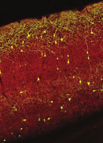
Research article                                                                                                     Neuroscience

                                        Head-to-head comparisons of electrophysiology and imaging data are rare in the literature, but
                                    are critically important as the practical aspects of each method affect their suitability for different
                                    experimental questions. Since the expression of calcium indicators can be restricted to genetically
                                    defined cell types, imaging can easily target recordings to specific sub-populations (Madisen et al.,
                                    2015). Similarly, the use of retro- or anterograde viral transfections to drive indicator expression
                                    allows imaging to target sub-populations defined by their projection patterns (Glickfeld et al.,
                                    2013; Gradinaru et al., 2010). The ability to identify genetically or projection-defined cell popula-
                                    tions in electrophysiology experiments is far more limited (Economo et al., 2018; Jia et al., 2019;
                                    Lima et al., 2009). Both techniques have been adapted for chronic recordings, but imaging offers
                                    the ability to reliably return to the same neurons over many days without the need to implant bulky
                                    hardware (Peters et al., 2014). Furthermore, because imaging captures structural, in addition to
                                    functional, data, individual neurons can be precisely registered to tissue volumes from electron
                                    microscopy (Bock et al., 2011; Lee et al., 2016), in vitro brain slices (Ko et al., 2011), and poten-
                                    tially other ex vivo techniques such as in situ RNA profiling (Chen et al., 2015). In contrast, the sour-
                                    ces of extracellular spike waveforms are very difficult to localize with sufficient precision to enable
                                    direct cross-modal registration.
                                        Inherent differences in the spatial sampling properties of electrophysiology and imaging are
                                    widely recognized, and influence what information can be gained from each method (Figure 1A).
                                    Multi-photon imaging typically yields data in a single plane tangential to the cortical surface, and is
                                    limited to depths of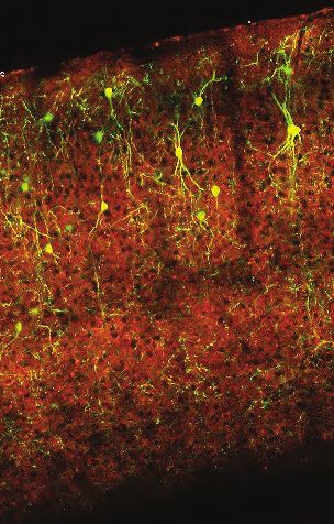
Research article Neuroscience
A 0 µm B
3 1
50
¬-- ¬--
neurons
250 0 0
Depth from
surface
500
50
neurons
1 mV
750
5s
Neuropixels Optical 5 ms
Electro- Projection
C physiology Tomography D
Transgenic Retinotopic
Mice Surgery Mapping Habituation
Two-Photon TissueCyte
Imaging
E
Gabors Full-Field Drifting Static Natural Natural Locally
Flashes Gratings Gratings Scenes Movies Sparse Noise
0 min 30 60 90 120 150
optotagging
0 min 30 60 0 min 30 60 0 min 30 60
Session A Session B Session C
F V1 LM AL PM AM
L2/3
L4
L5
L6
0 500 1000 0 500 1000 0 500 1000 0 500 1000 0 500 1000
L2/3
L4
L5
L6
0 5000 0 5000 0 5000 0 5000 0 5000
A Neuron count
AM
RL
AL PM Ephys Ephys + Imaging Imaging
LM Wild type Sst GCaMP6f Slc17a7 GCaMP6f Emx1 GCaMP6f Fezf2 GCaMP6f
V1
Pvalb ChR2 Vip GCaMP6f Cux2 GCaMP6f Rorb GCaMP6f Tlx3 GCaMP6f
Sst ChR2 Scnn1a GCaMP6f Rbp4 GCaMP6f
Vip ChR2 Nr5a1 GCaMP6f Ntsr1 GCaMP6f
Mouse visual cortex
(surface view)
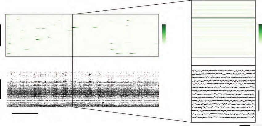
Figure 1. Overview of the ephys and imaging datasets. (A) Illustration of the orthogonal spatial sampling profiles of the two modalities. Black and white
area represents a typical imaging plane (at approximately 250 mm below the brain surface), while tan circles represent the inferred locations of cortical
neurons recorded with a Neuropixels probe (area is proportional to overall amplitude). (B) Comparison of temporal dynamics between the modalities.
Top: a heatmap of DF/F values for 100 neurons simultaneously imaged in V1 during the presentation of a 30 s movie clip. Bottom: raster plot for 100
Figure 1 continued on next page
Siegle, Ledochowitsch, et al. eLife 2021;10:e69068. DOI: https://doi.org/10.7554/eLife.69068 3 of 35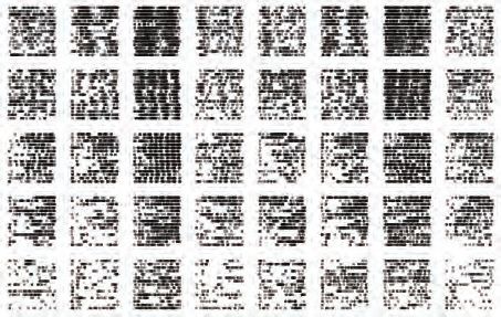
Research article                                                                                                                Neuroscience

Figure 1 continued
neurons simultaneously recorded with a Neuropixels probe in V1 in a different mouse viewing the same movie. Inset: Close-up of one sample of the
imaging heatmap, plotted on the same timescale as 990 samples from 15 electrodes recorded during the equivalent interval from the ephys
experiment. (C) Steps in the two data generation pipelines. Following habituation, mice proceed to either two-photon imaging or Neuropixels
electrophysiology. (D) Side-by-side comparison of the rigs used for ephys (left) and imaging (right). (E) Schematic of the stimulus set used for both
modalities. The ephys stimuli are shown continuously for a single session, while the imaging stimuli are shown over the course of three separate
sessions. (F) Histogram of neurons recorded in each area and layer, grouped by mouse genotype.

                                        Our comparison focused on metrics that capture three fundamental features of neural responses
                                     to environmental stimuli: (1) responsiveness, (2) preference (i.e. the stimulus condition that maxi-
                                     mizes the peak response), and (3) selectivity (i.e. sharpness of tuning). Responsiveness metrics char-
                                     acterize whether or not a particular stimulus type (e.g. drifting gratings) reproducibly elicits
                                     increased activity. For responsive neurons, preference metrics (e.g. preferred temporal frequency)
                                     determine which stimulus condition (out of a finite set) elicits the largest response, and serve as an
                                     indicator of a neuron’s functional specialization—for example, whether it responds preferentially to
                                     slow- or fast-moving stimuli. Lastly, selectivity metrics (e.g. orientation selectivity, lifetime sparse-
                                     ness) characterize a neuron’s ability to distinguish between particular exemplars within a stimulus
                                     class. All three of these features must be measured accurately in order to understand how stimuli
                                     are represented by individual neurons.
                                        We find that preference metrics are largely invariant across modalities. However, in this dataset,
                                     electrophysiology suggests that neurons show a higher degree of responsiveness, while imaging
                                     suggests that responsive neurons show a higher degree of selectivity. In the absence of steps taken
                                     to mitigate these differences, the two modalities will yield mutually incompatible conclusions about
                                     basic neural response properties. These differences could be reduced by lowering the amplitude
                                     threshold for valid DF/F events, applying a spikes-to-calcium forward model to the electrophysiology
                                     data (Deneux et al., 2016), or sub-selection of neurons based either on event rate or by contamina-
                                     tion level (the likelihood that signal from other neurons is misattributed to the neurons under consid-
                                     eration). This reconciliation reveals the respective biases of these two recording modalities, namely
                                     that extracellular electrophysiology predominantly captures the activity of highly active units while
                                     missing or merging low-firing-rate units, while calcium-indicator binding dynamics sparsify neural
                                     responses and supralinearly amplify spike bursts.

                                     Results
                                     We compared the visual responses measured in the Allen Brain Observatory Visual Coding (‘imag-
                                     ing’) and Allen Brain Observatory Neuropixels (‘ephys’) datasets, publicly available through brain-
                                     map.org and the AllenSDK Python package. These datasets consist of recordings from neurons in six
                                     cortical visual areas (as well as subcortical areas in the Neuropixels dataset) in the awake, head-fixed
                                     mouse in response to a battery of passively viewed visual stimuli. For both datasets, the same drift-
                                     ing gratings, static gratings, natural scenes, and natural movie stimuli were shown (Figure 1E). These
                                     stimuli were presented in a single 3 hr recording session for the ephys dataset. For the imaging data-
                                     set, these stimuli were divided across three separate 1 hr imaging sessions from the same group of
                                     neurons. In both ephys and imaging experiments, mice were free to run on a rotating disc, the
                                     motion of which was continuously recorded.
                                         The imaging dataset was collected using genetically encoded GCaMP6f (Chen et al., 2013) under
                                     the control of specific Cre driver lines. These Cre drivers limit the calcium indicator expression to
                                     specific neuronal populations, including different excitatory and inhibitory populations found in spe-
                                     cific cortical layers (see de Vries et al., 2020 for details). The ephys dataset also made use of trans-
                                     genic mice in addition to wild-type mice. These transgenic mice expressed either channelrhodopsin
                                     in specific inhibitory populations for identification using optotagging (see Siegle et al., 2021 for
                                     details), or GCaMP6f in specific excitatory or inhibitory populations (see Materials and methods).
                                     Unlike in the imaging dataset, however, these transgenic tools did not determine which neurons
                                     could be recorded.
                                         We limited our comparative analysis to putative excitatory neurons from five cortical visual areas
                                     (V1, LM, AL, PM, and AM). In the case of the imaging data, we only included data from 10 excitatory

Siegle, Ledochowitsch, et al. eLife 2021;10:e69068. DOI: https://doi.org/10.7554/eLife.69068                                                     4 of 35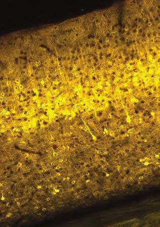
Research article                                                                                                     Neuroscience

                                    Cre lines, while for ephys we limited our analysis to regular-spiking units by setting a threshold on
                                    the waveform duration (>0.4 ms). After this filtering step, we were left with 41,578 neurons from 170
                                    mice in imaging, and 11,030 neurons from 52 mice in ephys. The total number of cells for each geno-
                                    type, layer, and area is shown in Figure 1F.

                                    Calculating response magnitudes for both modalities
                                    In order to directly compare results from ephys and imaging, we first calculated the magnitude of
                                    each neuron’s response to individual trials, which were defined as the interval over which a stimulus
                                    was present on the screen. We computed a variety of metrics based on these response magnitudes,
                                    and compared the overall distributions of those metrics for all the neurons in each visual area. The
                                    methods for measuring these responses necessarily differ between modalities, as explained below.
                                        For the ephys dataset, stimulus-evoked responses were computed using the spike times identi-
                                    fied by Kilosort2 (Pachitariu et al., 2016a; Stringer et al., 2019a). Kilosort2 uses information in the
                                    extracellularly recorded voltage traces to find templates that fit the spike waveform shapes of all the
                                    units in the dataset, and assigns a template to each spike. The process of ‘spike sorting’—regardless
                                    of the underlying algorithm—does not perfectly recover the true underlying spike times, and has the
                                    potential to miss spikes (false negatives) or assign spikes (or noise waveforms) to the wrong unit
                                    (false positives). The magnitude of the response for a given trial was determined by counting the
                                    total number of spikes (including false positives and excluding false negatives) that occured during
                                    the stimulation interval. This spike-rate–based analysis is the de facto standard for analyzing electro-
                                    physiology data, but it washes out information about bursting or other within-trial dynamics. For
                                    example, a trial that includes a four-spike burst will have the same apparent magnitude as a trial
                                    with four isolated spikes (Figure 2A).
                                        Methods for determining response magnitudes for neurons in imaging datasets are less standard-
                                    ized, and deserve careful consideration. The most commonly used approach involves averaging the
                                    continuous, baseline-normalized fluorescence signal over the trial interval. This method relies on
                                    information that is closer to the raw data. However, it suffers the severe drawback that, due to the
                                    long decay time of calcium indicators, activity from one trial can contaminate the fluorescence trace
                                    during the next trial, especially when relatively short (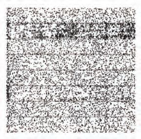
Research article Neuroscience
A visual input B grating phase
ground truth signal spike times [Ca2+]
spike burst
measured time series voltage trace ɣ--PU960
false positive
false negative
extracted events
1s 1s
response magnitude 4 4 10 1
C D
1 Hz 1 Hz
2 Hz preferred 2 Hz preferred
temporal temporal
4 Hz frequency 4 Hz frequency
8 Hz 8 Hz
15 Hz 15 Hz
2500 0 2500 Event 50 0 50
Spike count amplitude 0
0 global OSI: 0.26 global OSI: 0.82
preferred orientation preferred orientation
lifetime sparseness: 0.18 lifetime sparseness: 0.83
preferred
preferred
condition
condition 47% reliability
80% reliability
5 trials spont. threshold
5 trials spont. threshold
0 5 10
0 40 80 1s Trialwise
1s
Trialwise amplitude = 1 event amplitude
spike count
E Drifting Gratings Static Gratings Natural Scenes Natural Movies
1.0 1.0 1.0 1.0
0.32
Responsive fraction
0.31 0.28
0.8 0.17
0.17 0.21 0.24 0.8 0.8 0.8 0.32
0.23 0.17 0.31
0.29 0.22 0.31
0.2
0.6 0.6 0.21
0.24 0.6 0.2 0.6
0.23 0.24
0.4 0.4 0.4 0.4
0.2 0.2 0.2 0.2
0.0 0.0 0.0 0.0
V1 LM AL PM AM V1 LM AL PM AM V1 LM AL PM AM V1 LM AL PM AM
F V1 LM AL PM AM
D = 0.0517 D = 0.0352 D = 0.0162 D = 0.0334 D = 0.0419
1 2 4 8 15 Hz
Preferred temporal frequency
G V1 LM AL PM AM
D = 0.38 D = 0.41 D = 0.43 D = 0.46 D = 0.43
0.00 0.25 0.50 0.75 1.00
Lifetime sparseness
(Drifting Gratings)
Figure 2. Baseline metric comparison. (A) Steps involved in computing response magnitudes for units in the ephys dataset. (B) Same as A, but for the
imaging dataset. (C) Drifting gratings spike rasters for an example ephys neuron. Each raster represents 2 s of spikes in response to 15 presentations of
a drifting grating at one orientation and temporal frequency. Inset: spike raster for the neuron’s preferred condition, with each trial’s response
magnitude shown on the right, and compared to the 95th percentile of the spontaneous distribution. Responsiveness (purple), preference (red), and
Figure 2 continued on next page
Siegle, Ledochowitsch, et al. eLife 2021;10:e69068. DOI: https://doi.org/10.7554/eLife.69068 6 of 35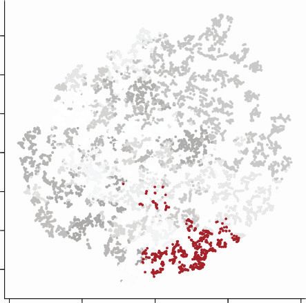
Research article                                                                                                               Neuroscience

Figure 2 continued
selectivity (brown) metrics are indicated. (D) Same as C, but for an example imaged neuron. (E) Fraction of neurons deemed responsive to each of four
stimulus types, using the same responsiveness metric for both ephys (gray) and imaging (green). Numbers above each pair of bars represent the
Jensen–Shannon distance between the full distribution of response reliabilities for each stimulus/area combination. (F) Distribution of preferred
temporal frequencies for all neurons in five different areas. The value D represents the Jensen–Shannon distance between the ephys and imaging
distributions. (G) Distributions of lifetime sparseness in response to a drifting grating stimulus for all neurons in five different areas. The value D
represents the Jensen–Shannon distance between the ephys and imaging distributions.
The online version of this article includes the following figure supplement(s) for figure 2:
Figure supplement 1. Baseline comparisons for additional preference and selectivity metrics.
Figure supplement 2. Matching laminar distribution patterns across modalities.
Figure supplement 3. Characterizing the impact of running behavior on response metrics.
Figure supplement 4. Matching running behavior across modalities.

                                     (Figure 2C) appears much denser than the corresponding event raster for a separate neuron that
                                     was imaged in the same area (Figure 2D). For each neuron, we computed responsiveness, prefer-
                                     ence, and selectivity metrics. We consider both neurons to be responsive to the drifting gratings
                                     stimulus class because they have a significant response (p < 0.05, compared to a distribution of
                                     activity taken during the epoch of spontaneous activity) on at least 25% of the trials of the preferred
                                     condition (the grating direction and temporal frequency that elicited the largest mean response)
                                     (de Vries et al., 2020). Since these neurons were deemed responsive according to this criterion,
                                     their function was further characterized in terms of their preferred stimulus condition and their selec-
                                     tivity (a measure of tuning curve sharpness). We use lifetime sparseness (Vinje and Gallant, 2000) as
                                     our primary selectivity metric, because it is a general metric that is applicable to every stimulus type.
                                     It reflects the distribution of responses of a neuron across some stimulus space (e.g. natural scenes
                                     or drifting gratings), equaling 0 if the neuron responds equivalently to all stimulus conditions, and
                                     one if the neuron only responds to a single condition. Across all areas and mouse lines, lifetime
                                     sparseness is highly correlated with more traditional selectivity metrics, such as drifting gratings ori-
                                     entation selectivity (R = 0.8 for ephys, 0.79 for imaging; Pearson correlation), static gratings orienta-
                                     tion selectivity (R = 0.79 for ephys, 0.69 for imaging), and natural scenes image selectivity (R = 0.85
                                     for ephys, 0.95 for imaging).
                                         For our initial analysis, we sought to compare the results from ephys and imaging as they are typi-
                                     cally analyzed in the literature, prior to any attempt at reconciliation. We will refer to these compari-
                                     sons as ‘baseline comparisons’ in order to distinguish them from subsequent comparisons made
                                     after applying one or more transformations to the imaging and/or ephys datasets. We pooled
                                     responsiveness, preference, and selectivity metrics for all of the neurons in a given visual area across
                                     experiments, and quantified the disparity between the imaging and ephys distributions using Jen-
                                     sen–Shannon distance. This is the square root of the Jensen–Shannon divergence, which is a method
                                     of measuring the disparity between two probability distributions that is symmetric and always has a
                                     finite value (Lin, 1991). Jensen–Shannon distance is equal to 0 for perfectly overlapping distribu-
                                     tions, and one for completely non-overlapping distributions, and falls in between these values for
                                     partially overlapping distributions.
                                         Across all areas and stimuli, the fraction of responsive neurons was higher in the ephys dataset
                                     than the imaging dataset (Figure 2E). To quantify the difference between modalities, we computed
                                     the Jensen–Shannon distance for the distributions of response reliabilities, rather than the fraction of
                                     responsive neurons at the 25% threshold level. This is done to ensure that our results are not too
                                     sensitive to the specific responsiveness threshold we have chosen. We found tuning preferences to
                                     be consistent between the two modalities, including preferred temporal frequency (Figure 2F), pre-
                                     ferred direction (Figure 2—figure supplement 1A), preferred orientation (Figure 2—figure supple-
                                     ment 1B), and preferred spatial frequency (Figure 2—figure supplement 1C). This was based on
                                     the qualitative similarity of their overall distributions, as well as their low values of Jensen–Shannon
                                     distance. Selectivity metrics, such as lifetime sparseness (Figure 2G), orientation selectivity (Fig-
                                     ure 2—figure supplement 1D), and direction selectivity (Figure 2—figure supplement 1E), were
                                     consistently higher in imaging than ephys.

Siegle, Ledochowitsch, et al. eLife 2021;10:e69068. DOI: https://doi.org/10.7554/eLife.69068                                                     7 of 35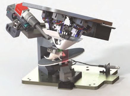
Research article                                                                                                    Neuroscience

                                    Controlling for laminar sampling bias and running behavior
                                    To control for potential high-level variations across the imaging and ephys experimental prepara-
                                    tions, we first examined the effect of laminar sampling bias. For example, the ephys dataset con-
                                    tained more neurons in layer 5, due to the presence of large, highly active cells in this layer. The
                                    imaging dataset, on the other hand, had more neurons in layer 4 due to the preponderance of layer
                                    4 Cre lines included in the dataset (Figure 2—figure supplement 2A). After resampling each data-
                                    set to match layer distributions (Figure 2—figure supplement 2B, see Materials and methods for
                                    details), we saw very little change in the overall distributions of responsiveness, preference, and
                                    selectivity metrics (Figure 2—figure supplement 2C–E), indicating that laminar sampling biases are
                                    likely not a key cause of the differences we observed between the modalities.
                                        We next sought to quantify the influence of behavioral differences on our comparison. As running
                                    and other motor behavior can influence visually evoked responses (Niell and Stryker, 2010;
                                    Stringer et al., 2019a; Vinck et al., 2015; de Vries et al., 2020), could modality-specific behavioral
                                    differences contribute to the discrepancies in the response metrics? In our datasets, mice tend to
                                    spend a larger fraction of time running in the ephys experiments, perhaps because of the longer
                                    experiment duration, which may be further confounded by genotype-specific differences in running
                                    behavior (Figure 2—figure supplement 3A). Within each modality, running had a similar impact on
                                    visual response metrics. On average, units in ephys and neurons in imaging have slightly lower
                                    responsiveness during periods of running versus non-running (Figure 2—figure supplement 3B),
                                    but slightly higher selectivity (Figure 2—figure supplement 3C). To control for the effect of running,
                                    we sub-sampled our imaging experiments in order to match the overall distribution of running frac-
                                    tion to the ephys data (Figure 2—figure supplement 4A). This transformation had a negligible
                                    impact on responsiveness, selectivity, and preference metrics (Figure 2—figure supplement 4B–D).
                                    From this analysis we conclude that, at least for the datasets examined here, behavioral differences
                                    do not account for the differences in functional properties inferred from imaging and ephys.

                                    Impact of event detection on functional metrics
                                    We sought to determine whether our approach to extracting events from the 2P data could explain
                                    between-modality differences in responsiveness and selectivity. Prior work has shown that scientific
                                    conclusions can depend on both the method of event extraction and the chosen parameters
                                    (Evans et al., 2019). However, the impact of different algorithms on functional metrics has yet to be
                                    assessed in a systematic way. To address this shortcoming, we first compared two event detection
                                    algorithms, exact ‘0 and unpenalized non-negative deconvolution (NND), another event extraction
                                    method that performs well on a ground truth dataset of simultaneous two-photon imaging and loose
                                    patch recordings from primary visual cortex (Huang et al., 2021). Care was taken to ensure that the
                                    characteristics of the ground truth imaging data matched those of our large-scale population record-
                                    ings in terms of their imaging resolution, frame rate, and noise levels, which implicitly accounted for
                                    differences in laser power across experiments.
                                        The correlation between the ground truth firing rate and the overall event amplitude within a
                                    given time bin is a common way of assessing event extraction performance (Theis et al., 2016;
                                    Berens et al., 2018; Rupprecht et al., 2021). Both algorithms performed equally well in terms of
                                    their ability to predict the instantaneous firing rate (for 100 ms bins, exact ‘0 r = 0.48 ± 0.23; NND r
                                    = 0.50 ± 0.24; p = 0.1, Wilcoxon signed-rank test). However, this metric does not capture all of the
                                    relevant features of the event time series. In particular, it ignores the rate of false positive events
                                    that are detected in the absence of a true underlying spike (Figure 3A). We found that the exact ‘0
                                    method, which includes a built-in sparsity constraint, had a low rate of false positives (8 ± 2% in 100
                                    ms bins, N = 32 ground truth recordings), whereas NND had a much higher rate (21 ± 4%; p = 8e-7,
                                    Wilcoxon signed-rank test). Small-amplitude false positive events have very little impact on the over-
                                    all correlation between the ground truth spike rate and the extracted events, so parameter optimiza-
                                    tion does not typically penalize such events. However, we reasoned that the summation of many
                                    false positive events could have a noticeable impact on response magnitudes averaged over trials.
                                    Because these events always have a positive sign, they cannot be canceled out by low-amplitude
                                    negative deflections of similar magnitude, as would occur when analyzing DF/F directly.
                                        We tested the impact of applying a minimum-amplitude threshold to the event time series
                                    obtained via NND. If the cumulative event amplitude within a given time bin (100 ms) did not exceed

Siegle, Ledochowitsch, et al. eLife 2021;10:e69068. DOI: https://doi.org/10.7554/eLife.69068                                         8 of 35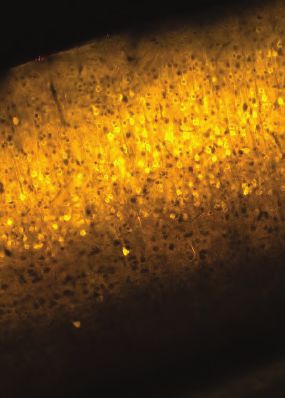
Research article Neuroscience
4
A
ɣ-- 2
.*H47
M[PTLZLYPLZ
0
6]LYHSSZ[H[PZ[PJZ
;Y\LZWPRL[PTLZ -PYPUNYH[L!
/a
,_HJ[ɥ0^P[OKLMH\S[˂
/P[YH[L!
,]LU[ 0.2 -HSZLWVZP[P]LYH[L!
HTWSP[\KL d̩!
0.0
5VUULNH[P]LKLJVU]VS\[PVU55+
/P[YH[L!
,]LU[ 0.2
-HSZLWVZP[P]LYH[L!
HTWSP[\KL d̩!
0.0
1s /P[
4PZZ
-HSZLWVZP[P]L
B C 1.0 D 0.30
N$JLSSZ^P[OZPT\S[HULV\Z
(]LYHNLYLZWVUZLYLSH[P]L
*VYYLSH[PVU^P[ONYV\UK[Y\[O
7HUKSVVZLWH[JO
-HSZLWVZP[P]LYH[L
0.20 TZIPUZPaL
0.4
0.3 0.4
0.10
0.2
0.2
0.1
0.0 0.0 0.00
0 2 4
10 0 2 4
10 0 2 4
10
;OYLZOVSKSL]LSˈ ;OYLZOVSKSL]LSˈ ;OYLZOVSKSL]LSˈ
E ˈ ˈ ˈ
,_HJ[ɥ0
KLMH\S[˂ 55+ N6:0$
F
N6:0$
.YH[PUNKPYLJ[PVU
ˈ ˈ
ˈ
,_HJ[ɥ
,WO`Z
0 20 40
0 20 40
;V[HSHTWSP[\KL ;V[HSHTWSP[\KL
0.12
HTWSP[\KL
UVJOHUNL
MPS[LY
N6:0$ N6:0$
[YPHSZ
ˈ
ˈ ˈ
0 20 40
0 20 40
;V[HSHTWSP[\KL
TZ ;V[HSHTWSP[\KL
0.00
1.00
3PML[PTLZWHYZLULZZ N$
:SJ
H
JLSSZMYVT=
KYPM[PUNNYH[PUNZ
G 1.0 +YPM[PUN.YH[PUNZ 1.0 :[H[PJ.YH[PUNZ 1.0 5H[\YHS:JLULZ
-YHJ[PVUVMYLZWVUZP]LJLSSZ
-YHJ[PVUVMYLZWVUZP]LJLSSZ
,WO`Z
-YHJ[PVUVMYLZWVUZP]LJLSSZ
,_HJ[ɥ0
0.4 0.4 0.4
0.2 0.2 0.2
0.0 0.0 0.0
0 2 4
10 0 2 4
10 0 2 4
10
;OYLZOVSKSL]LSˈ ;OYLZOVSKSL]LSˈ ;OYLZOVSKSL]LSˈ
Figure 3. Impact of calcium event detection on functional metrics. (A) GCaMP6f fluorescence trace, spike times, and detected events for one example
neuron with simultaneous imaging and electrophysiology. Events are either detected via exact ‘0-regularized deconvolution (Jewell and Witten, 2018)
or unpenalized non-negative deconvolution (Friedrich et al., 2017). Each 250 ms bin is classified as a ‘hit,’ ‘miss,’ ‘false positive,’ or ‘true positive’ by
comparing the presence/absence of detected events with the true underlying spike times. (B) Correlation between binned event amplitude and ground
Figure 3 continued on next page
Siegle, Ledochowitsch, et al. eLife 2021;10:e69068. DOI: https://doi.org/10.7554/eLife.69068 9 of 35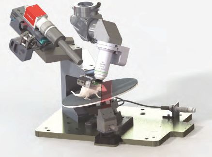
Research article                                                                                                                    Neuroscience

Figure 3 continued
truth firing rate after filtering NND events at different threshold levels relative to each neuron’s noise level (s). The average across neurons is shown as
colored dots. (C) Same as B, but for the average response amplitude within a 100 ms interval (relative to the amplitude with no thresholding applied).
(D) Same as B, but for the probability of detecting a false positive event in a 100 ms interval. (E) Event times in response to 600 drifting gratings
presentations for one example neuron, sorted by grating direction (ignoring differences in temporal frequency). Dots representing individual events are
scaled by the amplitude of the associated event. Each column represents the results of a different event detection method. The resulting tuning curves
and measured global orientation selectivity index (gOSI) are shown to the right of each plot. (F) Lifetime sparseness distributions for Scl17a7+ V1
neurons, after filtering out events at varying threshold levels relative to each neuron’s baseline noise level. The overall V1 distributions from ephys (gray)
and exact ‘0 (green) are overlaid on the most similar distribution. (G) Fraction of Slc17a7+ V1 neurons responding to three different stimulus types, after
filtering out events at varying threshold levels relative to each neuron’s baseline noise level.

                                      a threshold (set to a multiple of each neuron’s estimated noise level), the events in that window
                                      were removed. As expected, this procedure resulted in almost no change in the correlation between
                                      event amplitude and the ground truth firing rate (Figure 3B). However, it had a noticeable impact
                                      on both the average response magnitude within a given time window (Figure 3C), as well as the
                                      false positive rate (Figure 3D).
                                          Applying the same thresholding procedure to an example neuron from our population imaging
                                      dataset demonstrates how low-amplitude events can impact a cell’s apparent selectivity level. The
                                      prevalence of such events differs between the two compared approaches to event extraction, the
                                      exact ‘0 method used in Figure 2 and NND with no regularization (Figure 3E). When summing event
                                      amplitudes over many drifting gratings presentations, the difference in background rate has a big
                                      impact on the measured value of global orientation selectivity (gOSI), starting from 0.91 when using
                                      the exact ‘0 and dropping to 0.45 when using NND. However, these differences could be reconciled
                                      simply by setting a threshold to filter out low-amplitude events.
                                          Extracting events from a population dataset (N = 3095 Slc17a7+ neurons from V1) using NND
                                      resulted in much lower measured overall selectivity levels, even lower than for electrophysiology
                                      (Figure 3F). Thresholding out events at multiples of each neuron’s noise level (s) raised selectivity
                                      levels; a threshold between 3 and 4s brought the selectivity distribution closest to the ephys distri-
                                      bution, while a threshold between 4 and 5s resulted in selectivity that roughly matched that
                                      obtained with exact ‘0 (Figure 2G). The rate of low-amplitude events also affected responsiveness
                                      metrics (Figure 3G). Responsiveness was highest when all detected events were included, matching
                                      or slightly exceeding the levels measured with ephys. Again, applying an amplitude threshold
                                      between 4 and 5s brought responsiveness to the level originally measured with exact ‘0. By impos-
                                      ing the same noise-based threshold on the minimum event size that we originally computed to
                                      determine optimal regularization strength (essentially performing a post-hoc regularization), we are
                                      able to reconcile the results obtained with NND with those obtained via exact ‘0.
                                          This analysis demonstrates that altering the 2P event extraction methodology represents one pos-
                                      sible avenue for reconciling results from imaging and ephys. However, as different parameters were
                                      needed to reconcile either selectivity or responsiveness, and the optimal parameters further depend
                                      on the presented stimulus class, this cannot be the whole story. Furthermore, relying only on 2P
                                      event extraction parameters to reconcile results across modalities implies that the ephys data is itself
                                      unbiased, and all we need to do is adjust our imaging analysis pipeline until our metrics match.
                                      Because we know this is not the case, we explored the potential impacts of additional factors on the
                                      discrepancies between our ephys and imaging datasets.

                                      Controlling for transgene expression
                                      Given that imaging (but not ephys) approaches fundamentally require the expression of exogenous
                                      proteins (e.g. Cre, tTA, and GCaMP6f in the case of our transgenic mice) in specific populations of
                                      neurons, we sought to determine whether such foreign transgenes, expressed at relatively high lev-
                                      els, could alter the underlying physiology of the neural population. All three proteins have been
                                      shown to have neurotoxic effects under certain conditions (Han et al., 2012; Schmidt-Supprian and
                                      Rajewsky, 2007; Steinmetz et al., 2017), and calcium indicators, which by design bind intracellular
                                      calcium, can additionally interfere with cellular signaling pathways. To examine whether the expres-
                                      sion of these genes could explain the differences in functional properties inferred from imaging and
                                      ephys experiments, we performed electrophysiology in mice that expressed GCaMP6f under the

Siegle, Ledochowitsch, et al. eLife 2021;10:e69068. DOI: https://doi.org/10.7554/eLife.69068                                                         10 of 35
Research article Neuroscience
control of specific Cre drivers. We collected data from mice with GCaMP6f expressed in dense excit-
atory lines (Cux2 and Slc17a7) or in sparse inhibitory lines (Vip and Sst), and compared the results to
those obtained from wild-type mice (Figure 4A). On average, we recorded 45.9 ± 7.5 neurons per
area in 17 wild-type mice, and 55.8 ± 15.6 neurons per area in 19 GCaMP6f transgenic mice
(Figure 4B). The distribution of firing rates of recorded neurons in mice from all Cre lines was similar
to the distribution for units in wild-type mice (Figure 4C).
Because some GCaMP mouse lines have been known to exhibit aberrant seizure-like activity
(Steinmetz et al., 2017), we wanted to check whether spike bursts were more prevalent in these
mice. We detected bursting activity using the LogISI method, which identifies bursts in a spike train
based on an adaptive inter-spike interval threshold (Pasquale et al., 2010). The dense excitatory
Cre lines showed a slight increase in burst fraction (the fraction of all spikes that participate in bursts)
compared to wild-type mice (Figure 4D). This minor increase in burstiness, however, was not associ-
ated with changes in responsiveness or selectivity metrics that could account for the baseline differ-
ences between the ephys and imaging datasets. The fraction of responsive neurons was not lower in
the GCaMP6f mice, as it was for the imaging dataset—in fact, in some visual areas there was an
increase in responsiveness in the GCaMP6f mice compared to wild-type (Figure 4E). In addition, the
distribution of selectivities was largely unchanged between wild-type and GCaMP6f mice
(Figure 4F). Thus, while there may be subtle differences in the underlying physiology of GCaMP6f
mice, particularly in the dense excitatory lines, those differences cannot explain the large discrepan-
cies in visual response metrics derived from ephys or imaging.
Forward-modeling synthetic imaging data from experimental ephys
data
Given the substantial differences between the properties of extracellularly recorded spikes and
events extracted from fluorescence traces (Figure 2A–C), and the potential impact of event extrac-
tion parameters on derived functional metrics (Figure 3), we hypothesized that transforming spike
trains into simulated calcium events could reconcile some of the baseline differences in response
metrics we have observed. The inverse transformation—converting fluorescence events into syn-
thetic spike times—is highly under-specified, due to the reduced temporal resolution of calcium
imaging (Figure 1B).
To implement the spikes-to-calcium transformation, we used MLSpike, a biophysically inspired
forward model (Deneux et al., 2016). MLSpike explicitly considers the cooperative binding between
GCaMP and calcium to generate synthetic DF/F fluorescence traces using the spike trains for each
unit recorded with ephys as input. We extracted events from these traces using the same exact ‘0-
regularized detection algorithm applied to our experimental imaging data, and used these events as
inputs to our functional metrics calculations (Figure 5A).
A subset of the free parameters in the MLSpike model (e.g. DF/F rise time, Hill parameter, satura-
tion parameter, and normalized resting calcium concentration) were fit to simultaneously acquired
loose patch and two-photon-imaging recordings from layer 2/3 of mouse visual cortex
(Huang et al., 2021). Additionally, three parameters were calibrated on the fluorescence traces from
the imaging dataset to capture the neuron-to-neuron variance of these parameters: the average
amplitude of a fluorescence transient in response to a spike burst (A), the decay time of the fluores-
cence transients (t ), and the level of Gaussian noise in the signal (s) (Figure 5B). For our initial char-
acterization, we selected parameter values based on the mode of the overall distribution from the
imaging dataset.
The primary consequence of the forward model was to ‘sparsify’ each neuron’s response by wash-
ing out single spikes while non-linearly boosting the amplitude of ‘bursty’ spike sequences with short
inter-spike intervals. When responses were calculated on the ephys spike train, a trial containing a 4-
spike burst within a 250 ms window would have the same magnitude as a trial with four isolated
spikes across the 2 s trial. After the forward model, however, the burst would be transformed into
an event with a magnitude many times greater than the events associated with isolated spikes, due
to the nonlinear relationship between spike counts and the resulting calcium-dependent fluores-
cence. This effect can be seen in stimulus-locked raster plots for the same neuron before and after
applying the forward model (Figure 5C).
What effects does this transformation have on neurons’ inferred functional properties? Applying
the forward model plus event extraction to the ephys data did not systematically alter the fraction of
Siegle, Ledochowitsch, et al. eLife 2021;10:e69068. DOI: https://doi.org/10.7554/eLife.69068 11 of 35Research article Neuroscience
A B
160
140
120
Unit count (after QC)
100
80
60
Sst Vip Slc17a7 Cux2 40
20
Wild type Sst GCaMP6f Slc17a7 GCaMP6f
Vip GCaMP6f Cux2 GCaMP6f 0
V1 LM AL PM AM
C V1 LM AL PM AM
0.056 0.067 0.081 0.092 0.032
0.079 0.056 0.098 0.094 0.048
0.096 0.081 0.072 0.065 0.101
0.062 0.096 0.105 0.083
0.01 0.1 1 10 100
Firing rate (Hz)
D
0.149 0.091 0.14 0.105 0.146
0.204 0.131 0.148 0.103
0.125 0.068 0.076 0.145 0.086
0.121 0.08 0.108 0.138 0.1
0.05 0.5 1.0
Burst fraction
E 1.0
0.081 0.147 0.093 0.108 0.117 0.089 0.104 0.089 0.091 0.111 0.094 0.178 0.068 0.084 0.073 0.083 0.081 0.127 0.137
0.8
Responsive fraction
(Drfiting Gratings)
0.6
0.4
0.2
0.0
F
0.1 0.15 0.19 0.13 0.16
0.12 0.12 0.16 0.13 0.14
0.11 0.15 0.14 0.07 0.15
0.12 0.13 0.12 0.09
0.0 0.5 1.0
Lifetime sparseness
(Drifting Gratings)
Figure 4. Comparing responses across GCaMP-expressing mouse lines. (A) GCaMP expression patterns for the four lines used for ephys experiments,
based on two-photon serial tomography (TissueCyte) sections from mice used in the imaging pipeline. (B) Unit yield (following QC filtering) for five
areas and five genotypes. Error bars represent standard deviation across experiments; each dot represents a data point from one experiment. (C)
Distribution of firing rates for neurons from each mouse line, aggregated across experiments. (D) Distribution of burst fraction (fraction of all spikes that
Figure 4 continued on next page
Siegle, Ledochowitsch, et al. eLife 2021;10:e69068. DOI: https://doi.org/10.7554/eLife.69068 12 of 35Research article Neuroscience
Figure 4 continued
participate in bursts) for neurons from each mouse line, aggregated across experiments. Dots represent the median of each distribution, shown in
relation to a reference value of 0.3. (E) Fraction of neurons deemed responsive to drifting gratings, grouped by genotype. (F) Distribution of lifetime
sparseness in response to a drifting grating stimulus, grouped by genotype. In panels (C–F), colored numbers indicate the Jensen–Shannon distance
between the wild-type distribution and the distributions of the four GCaMP-expressing mouse lines. Area PM does not include data from Cux2 mice, as
it was only successfully targeted in one session for this mouse line.
responsive units in the dataset. While 8% of neurons switched from being responsive to drifting gra-
tings to unresponsive, or vice versa, they did so in approximately equal numbers (Figure 5D). The
forward model did not improve the match between the distributions of response reliabilities (our
responsiveness metric) for any stimulus type (Figure 5E). The forward model similarly had a negligi-
ble impact on preference metrics; for example, only 14% of neurons changed their preferred tempo-
ral frequency after applying the forward model (Figure 5F), and the overall distribution of preferred
temporal frequencies still matched that from the imaging experiments (Figure 5G). In contrast,
nearly all neurons increased their selectivity after applying the forward model (Figure 5H). Overall,
the distribution of lifetime sparseness to drifting gratings became more similar to—but still did not
completely match—the imaging distribution across all areas (Figure 5I). The average Jensen–Shan-
non distance between the ephys and imaging distributions was 0.41 before applying the forward
model, compared to 0.14 afterward (mean bootstrapped distance between the sub-samples of the
imaging distribution = 0.064; p < 0.001 for all areas, since 1000 bootstrap samples never exceeded
the true Jensen–Shannon distance; see Materials and methods for details). These results imply that
the primary effects of the forward model—providing a supralinear boost to the ‘amplitude’ of spike
bursts, and thresholding out single spike events—can account for baseline differences in selectivity,
but not responsiveness, between ephys and imaging.
To assess whether the discrepancies between the imaging and ephys distributions of responsive-
ness and selectivity metrics could be further reduced by using a different set of forward model
parameters, we brute-force sampled 1000 different parameter combinations for one ephys session,
using 10 values each for amplitude, decay time, and noise level (Figure 5—figure supplement 1A),
spanning the entire range of parameters calibrated on the experimental imaging data. The fraction
of responsive neurons did not change as a function of forward model parameters, except for the
lowest values of amplitude and noise level, where it decreased substantially (Figure 5—figure sup-
plement 1B). This parameter combination (A 0.0015, sigma 0.03) was observed in less than 1%
of actual neurons recorded with two-photon imaging, so it cannot account for differences in respon-
siveness between the two modalities. Both the difference between the median lifetime sparseness
for imaging and ephys, as well as the Jensen–Shannon distance between the full ephys and imaging
lifetime sparseness distributions, were near the global minimum for the parameter values we initially
used (Figure 5—figure supplement 1C,D).
It is conceivable that the inability of the forward model to fully reconcile differences in responsive-
ness and selectivity was due to the fact that we applied the same parameters across all neurons of
the ephys dataset, without considering their genetically defined cell type. To test for cell-type-spe-
cific differences in forward model parameters, we examined the distributions of amplitude, decay
time, and noise level for individual excitatory Cre lines used in the imaging dataset. The distributions
of parameter values across genotypes were largely overlapping, with the exception of increasing
noise levels for some of the deeper populations (e.g. Tlx3-Cre in layer 5, and Ntsr1-Cre_GN220 in
layer 6) and an abundance of low-amplitude neurons in the Fezf2-CreER population (Figure 5—fig-
ure supplement 2A). Given that higher noise levels and lower amplitudes did not improve the corre-
spondence between the ephys and imaging metric distributions, we concluded that selecting
parameter values for individual neurons based on their most likely cell type would not change our
results. Furthermore, we saw no correlation between responsiveness or selectivity metrics in imaged
neurons and their calibrated amplitude, decay time, or noise level (Figure 5—figure supplement
2B–E).
Effect of ephys selection bias
We next sought to determine whether electrophysiology’s well-known selection bias in favor of
more active neurons could account for the differences between modalities. Whereas calcium
Siegle, Ledochowitsch, et al. eLife 2021;10:e69068. DOI: https://doi.org/10.7554/eLife.69068 13 of 35Research article Neuroscience
A
Original spike train
200%
¬--
:PT\SH[LKɣ--
ɥ0 events
5s
ORIGINAL AFTER FORWARD MODEL
B Spike burst C
Amplitude :PT\SH[LKɣ--[YHJL
(A)
20 trials
Noise level
(ˈ)
+LJH`[PTL
(ˉ) 0 2 0 20 0 2 0 5
Time (s) Overall magnitude Time (s) Overall magnitude
D Responsive? E
Drifting Gratings :[H[PJ.YH[PUNZ 5H[\YHS:JLULZ
1.0 1.0 1.0
0.32
9LZWVUZP]LMYHJ[PVU
2000 YES 0.8 0.16 0.19
0.8 0.8 0.2
0.15 0.23 0.26
0.22 0.3
units 0.23
0.23
0.6 0.6 0.26 0.6 0.23
0.24
0.26
0.4 0.4 0.4
NO 0.2 0.2 0.2
Original After 0.0 0.0 0.0
forward model V1 LM AL PM AM V1 LM AL PM AM V1 LM AL PM AM
Experimental 2P imaging
:`U[OL[PJ7PTHNPUN
F 7YLMLYYLK[LTWVYHSMYLX\LUJ` G
1 V1 LM AL PM AM
After forward model
# of units
2
2000
D = 0.0463 D = 0.0348 D = 0.0144 D = 0.0213 D = 0.0529
4
1000
8 0
15
1 2 4 8 15 Hz
1 2 4 8 15 Hz 7YLMLYYLK[LTWVYHSMYLX\LUJ`
Original
Lifetime sparseness
H (Drifting Gratings) I
1.0
V1 LM AL PM AM
After forward model
0.8
0.6
0.4
D = 0.12 D = 0.15 D = 0.15 D = 0.17 D = 0.15
0.2 0.0 0.5 1.0
0.0 Lifetime sparseness
0.0 0.2 0.4 0.6 0.8 1.0 (Drifting Gratings)
Original
Figure 5. Effects of the spikes-to-calcium forward model. (A) Example of the forward model transformation. A series of spike times (top) is converted to
a simulated DF/F trace (middle), from which ‘0-regularized events are extracted using the same method as for the experimental imaging data (bottom).
(B) Overview of the three forward model parameters that were fit to data from the Allen Brain Observatory two-photon imaging experiments. (C) Raster
plot for one example neuron, before and after applying the forward model. Trials are grouped by drifting grating direction and ordered by response
Figure 5 continued on next page
Siegle, Ledochowitsch, et al. eLife 2021;10:e69068. DOI: https://doi.org/10.7554/eLife.69068 14 of 35Research article Neuroscience
Figure 5 continued
magnitude from the original ephys data. The magnitudes of each trial (based on ephys spike counts or summed imaging event amplitudes) are shown
to the right of each plot. (D) Count of neurons responding (green) or not responding (red) to drifting gratings before or after applying the forward
model. (E) Fraction of neurons deemed responsive to each of three stimulus types, for both synthetic fluorescence traces (yellow) and true imaging data
(green). Numbers above each pair of bars represent the Jensen–Shannon distance between the full distribution of responsive trial fractions for each
stimulus/area combination. (F) 2D histogram of neurons’ preferred temporal frequency before and after applying the forward model. (G) Distribution of
preferred temporal frequencies for all neurons in five different areas. The Jensen–Shannon distance between the synthetic imaging and true imaging
distributions is shown for each plot. (H) Comparison between measured lifetime sparseness in response to drifting grating stimulus before and after
applying the forward model. (I) Distributions of lifetime sparseness in response to a drifting grating stimulus for all neurons in five different areas. The
Jensen–Shannon distance between the synthetic imaging and true imaging distributions is shown for each plot.
The online version of this article includes the following figure supplement(s) for figure 5:
Figure supplement 1. Sampling the entire space of forward model parameters.
Figure supplement 2. Relationship between forward model parameters, genotype, and functional metrics.
imaging can detect the presence of all neurons in the field of view that express a fluorescent indica-
tor, ephys cannot detect neurons unless they fire action potentials. This bias is exacerbated by the
spike sorting process, which requires a sufficient number of spikes in order to generate an accurate
template of each neuron’s waveform. Spike sorting algorithms can also mistakenly merge spikes
from nearby neurons into a single ‘unit’ or allow background activity to contaminate a spike train,
especially when spike waveforms generated by one neuron vary over time, for example due to the
adaptation that occurs during a burst. These issues all result in an apparent activity level increase in
ephys recordings. In addition, assuming a 50-mm ‘listening radius’ for the probes (radius of half-cylin-
der around the probe where the neurons’ spike amplitude is sufficiently above noise to trigger
detection) (Buzsáki, 2004; Harris et al., 2016; Shoham et al., 2006), the average yield of 116 regu-
lar-spiking units/probe (prior to QC filtering) would imply a density of 42,000 neurons/mm3, much
lower than the known density of ~90,000 neurons/mm3 for excitatory cells in mouse visual cortex
(Erö et al., 2018).
If the ephys dataset is biased toward recording neurons with higher firing rates, it may be more
appropriate to compare it with only the most active neurons in the imaging dataset. To test this, we
systematically increased the event rate threshold for the imaged neurons, so the remaining neurons
used for comparison were always in the upper quantile of mean event rate. Applying this filter
increased the overall fraction of responsive neurons in the imaging dataset, such that the experimen-
tal imaging and synthetic imaging distributions had the highest similarity when between 7 and 39%
of the most active imaged neurons were included (V1: 39%, LM: 34%, AL: 25%, PM: 7%, AM: 14%)
(Figure 6A). This indicates that more active neurons tend to be more responsive to our visual stimuli,
which could conceivably account for the discrepancy in overall responsiveness between the two
modalities. However, applying this event rate threshold actually increased the differences between
the selectivity distributions, as the most active imaged neurons were also more selective (Figure 6B).
Thus, sub-selection of imaged neurons based on event rate was not sufficient to fully reconcile the
differences between ephys and imaging. Performing the same analysis using sub-selection based on
the coefficient of variation, an alternative measure of response reliability, yielded qualitatively similar
results (Figure 6—figure supplement 1).
If the ephys dataset includes spike trains that are contaminated with spurious spikes from one or
more nearby neurons then it may help to compare our imaging results only to the least contami-
nated neurons from the ephys dataset. Our initial QC process excluded units with an inter-spike
interval (ISI) violations score (Hill et al., 2011, see Materials and methods for definition) above 0.5,
to remove highly contaminated units, but while the presence of refractory period violations implies
contamination, the absence of such violations does not imply error-free clustering, so some contami-
nation may remain. We systematically decreased our tolerance for ISI-violating ephys neurons, so the
remaining neurons used for comparison were always in the lower quantile of contamination level.
For the most restrictive thresholds, where there was zero detectable contamination in the original
spike trains (ISI violations score = 0), the match between the synthetic imaging and experimental
imaging selectivity and responsiveness distributions was maximized (Figure 6C,D). This indicates
that, unsurprisingly, contamination by neighboring neurons (as measured by ISI violations score)
reduces selectivity and increases responsiveness. Therefore, the inferred functional properties are
Siegle, Ledochowitsch, et al. eLife 2021;10:e69068. DOI: https://doi.org/10.7554/eLife.69068 15 of 35Research article Neuroscience
A B
0.70
Median lifetime sparseness
0.80
Fraction responsive
0.65
0.75
0.60 0.70
0.55 0.65
0.50 0.60
0.45 0.55
100% 80% 60% 40% 20% 0% 100% 80% 60% 40% 20% 0%
0.5 Imaged neurons included 0.5 Imaged neurons included
0.4 0.4
J-S distance
J-S distance
0.3 0.3
0.2 0.2
0.1 0.1
0.0 0.0
100% 80% 60% 40% 20% 0% 100% 80% 60% 40% 20% 0%
V1
filter direction LM
AL
PM
0.1 1.0 AM 0.1 1.0
Event rate (Hz) Event rate (Hz)
C D
0.80 0.80
Median lifetime sparseness
Fraction responsive
0.70 0.70
0.60 0.60
0.50 0.50
0.40 0.40
100% 80% 60% 40% 20% 0% 100% 80% 60% 40% 20% 0%
0.30 Ephys neurons included 0.30 Ephys neurons included
J-S distance
J-S distance
0.20 0.20
0.10 0.10
0.00 0.00
100% 80% 60% 40% 20% 0% 100% 80% 60% 40% 20% 0%
filter direction
V1
LM
AL
PM
0 0.0001 0.001 0.01 0.1 AM
0 0.0001 0.001 0.01 0.1
ISI violations score ISI violations score
Figure 6. Sub-sampling based on event rate or ISI violations. (A) Top: Change in fraction of neurons responding to drifting gratings for each area in the
imaging dataset, as function of the percent of imaged neurons included in the comparison. Middle: Jensen–Shannon distance between the synthetic
imaging and true imaging response reliability distributions. Bottom: Overall event rate distribution in the imaging dataset. As the percentage of
included neurons decreases (from left to right), more and more neurons with low activity rates are excluded. (B) Same as A, but for drifting gratings
Figure 6 continued on next page
Siegle, Ledochowitsch, et al. eLife 2021;10:e69068. DOI: https://doi.org/10.7554/eLife.69068 16 of 35Research article Neuroscience
Figure 6 continued
lifetime sparseness (selectivity) metrics. (C) Top: Change in fraction of neurons responding to the drifting gratings stimulus for each area in the ephys
dataset, as function of the percent of ephys neurons included in the comparison. Middle: Jensen–Shannon distance between the synthetic imaging and
true imaging response reliability distributions. Bottom: Overall ISI violations score distribution in the ephys dataset. As the percent of included neurons
decreases (from right to left), more and more neurons with high contamination levels are excluded. Yellow shaded area indicates the region where the
minimum measurable contamination level (ISI violations score = 0) is reached. (D) Same as C, but for drifting gratings lifetime sparseness (selectivity)
metrics.
The online version of this article includes the following figure supplement(s) for figure 6:
Figure supplement 1. An alternative metric of response robustness.
most congruent across modalities when the ephys analysis includes a stringent threshold on the max-
imum allowable contamination level.
Results across stimulus types
The previous results have primarily focused on the drifting gratings stimulus, but we observe similar
effects for all of the stimulus types shared between the imaging and ephys datasets. Figure 7 sum-
marizes the impact of each transformation we performed, either before or after applying the forward
model, for drifting gratings, static gratings, natural scenes, and natural movies.
Across all stimulus types, the forward model had very little impact on responsiveness. Instead,
sub-selecting the most active neurons from our imaging experiments using an event-rate filter ren-
dered the shape of the distributions the most similar. For the stimulus types for which we could mea-
sure preference across small number of categories (temporal frequency of drifting gratings and
spatial frequency of static gratings), no data transformations were able to improve the overall match
between the ephys and imaging distributions, as they were already very similar in the baseline com-
parison. For selectivity metrics (lifetime sparseness), applying the forward model played the biggest
role in improving cross-modal similarity, although there was a greater discrepancy between the
resulting distributions for static gratings, natural scenes, and natural movies than there was for drift-
ing gratings. Filtering ephys neurons based on ISI violations further reduced the Jensen–Shannon
distance, but it still remained well above zero. This indicates that the transformations we employed
could not fully reconcile observed differences in selectivity distributions between ephys and
imaging.
Lessons for future comparisons
Our study shows that population-level functional metrics computed from imaging and electrophysi-
ology experiments can display systematic biases. What are the most important takeaways that
should be considered for those performing similar comparisons?
Preference metrics are similar across modalities
At least for the cell population we considered (putative excitatory neurons from all layers of visual
cortex), preference metrics (such as preferred temporal frequency, preferred spatial frequency, and
preferred direction) were largely similar between imaging and electrophysiology (Figure 2F, Fig-
ure 2—figure supplement 1A–C). Because these are categorical metrics defined as the individual
condition (out of a finite set) that evokes the strongest mean response, they are robust to the choice
of calcium event extraction method and also remain largely invariant to the application of a spikes-
to-calcium forward model to electrophysiology data. One caveat to keep in mind is that when imag-
ing from more specific populations (e.g. using a transgenic line that limits imaging to a specific sub-
type of neuron in a specific layer), electrophysiology experiments may yield conflicting preference
metrics unless the sample is carefully matched across modalities (e.g. by genetically tagging electri-
cally recorded neurons with a light-sensitive opsin).
Siegle, Ledochowitsch, et al. eLife 2021;10:e69068. DOI: https://doi.org/10.7554/eLife.69068 17 of 35You can also read