FAIRV2.0.0: A GENERALIZED IMPULSE RESPONSE MODEL FOR CLIMATE UNCERTAINTY AND FUTURE SCENARIO EXPLORATION - GMD
←
→
Page content transcription
If your browser does not render page correctly, please read the page content below
Geosci. Model Dev., 14, 3007–3036, 2021
https://doi.org/10.5194/gmd-14-3007-2021
© Author(s) 2021. This work is distributed under
the Creative Commons Attribution 4.0 License.

FaIRv2.0.0: a generalized impulse response model for climate
uncertainty and future scenario exploration
Nicholas J. Leach1 , Stuart Jenkins1 , Zebedee Nicholls2,3 , Christopher J. Smith4,5 , John Lynch1 , Michelle Cain1 ,
Tristram Walsh1 , Bill Wu1 , Junichi Tsutsui6 , and Myles R. Allen1,7
1 Atmospheric,   Oceanic, and Planetary Physics, Department of Physics, University of Oxford, Oxford, UK
2 Australian–German     Climate and Energy College, University of Melbourne, Melbourne, Australia
3 School of Geography, Earth and Atmospheric Sciences, University of Melbourne, Melbourne, Australia
4 School of Earth and Environment, University of Leeds, Leeds, UK
5 International Institute for Applied Systems Analysis, Laxenburg, Austria
6 Environmental Science Research Laboratory, Central Research Institute of Electric Power Industry, Abiko, Japan
7 Environmental Change Institute, University of Oxford, Oxford, UK

Correspondence: Nicholas J. Leach (nicholas.leach@stx.ox.ac.uk) and Christopher J. Smith (c.j.smith1@leeds.ac.uk)

Received: 20 November 2020 – Discussion started: 24 November 2020
Revised: 13 April 2021 – Accepted: 14 April 2021 – Published: 27 May 2021

Abstract. Here we present an update to the FaIR model for         plex models) are not themselves intrinsically biased “hot”
use in probabilistic future climate and scenario exploration,     or “cold”: it is the choice of parameters and how those are
integrated assessment, policy analysis, and education. In this    selected that determines the model response, something that
update we have focussed on identifying a minimum level            appears to have been misunderstood in the past. This updated
of structural complexity in the model. The result is a set of     FaIR model is able to reproduce the global climate system
six equations, five of which correspond to the standard im-       response to GHG and aerosol emissions with sufficient accu-
pulse response model used for greenhouse gas (GHG) met-           racy to be useful in a wide range of applications and therefore
ric calculations in the IPCC’s Fifth Assessment Report, plus      could be used as a lowest-common-denominator model to
one additional physically motivated equation to represent         provide consistency in different contexts. The fact that FaIR
state-dependent feedbacks on the response timescales of each      can be written down in just six equations greatly aids trans-
greenhouse gas cycle. This additional equation is necessary       parency in such contexts.
to reproduce non-linearities in the carbon cycle apparent in
both Earth system models and observations. These six equa-
tions are transparent and sufficiently simple that the model is
able to be ported into standard tabular data analysis packages,   1   Introduction
such as Excel, increasing the potential user base consider-
ably. However, we demonstrate that the equations are flexible     Earth system models (ESMs) are vital tools for providing in-
enough to be tuned to emulate the behaviour of several key        sight into the drivers behind Earth’s climate system, as well
processes within more complex models from CMIP6. The              as projecting impacts of future emissions. Large scale multi-
model is exceptionally quick to run, making it ideal for inte-    model studies, such as the Coupled Model Intercomparison
grating large probabilistic ensembles. We apply a constraint      Projects (Eyring et al., 2016; Taylor et al., 2012, CMIPs),
based on the current estimates of the global warming trend        have been used in many reports to produce projections of
to a million-member ensemble, using the constrained ensem-        what the future climate may look like based on a range of
ble to make scenario-dependent projections and infer ranges       different concentration scenarios, with associated emission
for properties of the climate system. Through these analyses,     scenarios and socio-economic narratives quantified by inte-
we reaffirm that simple climate models (unlike more com-          grated assessment models (IAMs). In addition to simulating
                                                                  both the past and possible future climates, these CMIPs ex-

Published by Copernicus Publications on behalf of the European Geosciences Union.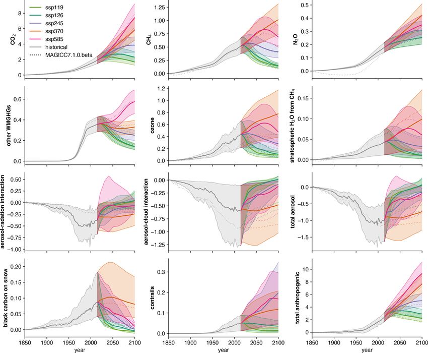
3008                                                                                                  N. J. Leach et al.: FaIRv2.0.0

tensively use idealized experiments to try to determine some            SCMs. In the past, this has led to different simple models
of the key properties of the climate system, such as the equi-          being used by different working groups in major reports, re-
librium climate sensitivity (ECS, Collins et al., 2013) or the          ducing the consistency of the overall work. We believe one
transient climate response to cumulative carbon emissions               key step towards a transparent and coherent process in IPCC
(Allen et al., 2009, TCRE).                                             assessments would be to use at least one common SCM as
   While ESMs are integral to our current understanding of              widely as possible throughout all working groups, allowing
how the climate system responds to greenhouse gas (GHG)                 results to be directly comparable. Such use would provide ad-
and aerosol emissions and provide the most comprehensive                ditional context alongside domain-specific models. For this
projections of what a future world might look like, they are            to be realized, an SCM that is both easy to understand and
so computationally expensive that only a limited set of ex-             adapt is required.
periments are able to be run during a CMIP. This constraint                An important innovation of the IPCC 5th Assessment Re-
on the quantity of experiments necessitates the use of sim-             port (Myhre et al., 2013) was the introduction of a transparent
pler models to provide probabilistic assessments and explore            set of equations (the AR5-IR model) for use in the calculation
additional experiments and scenarios. These models, often               of GHG metrics. However, that model was not quite adequate
referred to as simple climate models (SCMs), are typically              to reproduce the evolution of the integrated impulse response
designed to emulate the response of more complex mod-                   to emissions over time, due to the lack of non-linearity in the
els. In general, they are able to simulate the globally aver-           carbon cycle. The Finite amplitude Impulse Response (FaIR)
aged emission → concentration → radiative forcing → tem-                model v1.0 (Millar et al., 2017) introduced a state depen-
perature response pathway and can be tuned to emulate an                dence to the AR5-IR carbon cycle. This state-dependent car-
individual ESM (or multi-model mean). In general, SCMs                  bon cycle was better able to capture both the observed rela-
are considerably less complex than ESMs: while ESMs are                 tionship between historical emission trajectories and atmo-
three dimensional, gridded, and explicitly represent dynam-             spheric CO2 burden and the behaviour of ESMs in idealized
ical and physical processes, therefore outputting many hun-             concentration increase and pulse emission experiments. FaIR
dreds of variables, SCMs tend to be globally averaged (or               v1.0 used four equations to model the atmospheric gas cycle
cover large regions) and parameterize many processes, re-               and corresponding effective radiative forcing (ERF) impact
sulting in many fewer output variables. This reduction in               of CO2 and a further two (unchanged from the AR5-IR) to
complexity means that SCMs are much quicker than ESMs                   emulate the climate system’s thermal response to changes in
in terms of runtime: most SCMs can run tens of thousands                ERF. Subsequently, Smith et al. (2018) added a representa-
of years of simulation per minute on an “average” personal              tion of other GHGs and aerosols, which necessarily increased
computer, whereas ESMs may take several hours to run a                  the structural complexity of the model in FaIRv1.3. In this
single year on hundreds of supercomputer processors. Most               update, we maintain the ability to simulate the atmospheric
SCMs are also much smaller in terms of the number of lines              response to a wide range of GHGs and aerosol emissions,
of code: SCMs tend to be on the order of thousands of lines,            while attempting to significantly reduce the complexity of
while ESMs can be up to a million lines (Alexander and East-            the model structure.
erbrook, 2015).                                                            In FaIRv2.0.0 we propose a set of six equations that we
   There are many simple climate models (Nicholls et al.,               demonstrate are sufficient to capture the global mean climate
2020a) that have been in use by the climate science and in-             system response to GHG and aerosol emissions. These six
tegrated assessment modelling communities for decades. Of               equations are outlined in Fig. 1. In this text we explain the
particular note are MAGICC (Meinshausen et al., 2011a),                 physical reasoning behind each equation and select a default
which has dominated SCM usage within integrated assess-                 parameter set based on simple tunings to historical observa-
ment models, and FaIR1 (Smith et al., 2018), both of which              tions and recent literature. We compare the default response
were used in the Intergovernmental Panel on Climate Change              of FaIRv2.0.0 to a publicly available version of the widely
(IPCC) Special Report on 1.5 ◦ C warming (IPCC, 2018,                   used SCM, MAGICC6 (Meinshausen et al., 2011a, b), for a
SR15). However, while these models are “simple” in com-                 range of socioeconomic pathways (Riahi et al., 2017, SSPs).
parison to the ESMs they emulate, they are often not simple             Further, we show that these equations can be tuned to emu-
enough to allow new users to gain enough familiarity with the           late key properties of a range of CMIP6 (Eyring et al., 2016)
underlying equations to understand their behaviour without              models. Finally, we constrain a large parameter ensemble in-
significant effort. This learning curve reduces their uptake by         ferred from more complex models and contemporary assess-
the wider community, and has resulted in different research             ments with observations of the present-day warming level
groups generally using the single model that they are most              and rate to provide a set of observationally constrained prob-
familiar with (Nicholls et al., 2020a) from the wide range of           abilistic projections for the future climate following (Smith
                                                                        et al., 2018).
    1 We refer to the FaIR model in general as “FaIR”, to the version      FaIRv2.0.0 is sufficiently simple as to be able to be used
presented in this text as “FaIRv2.0.0”, and to the specific implemen-   in undergraduate and high-school teaching of climate change
tation used to create the figures as “FaIRv2.0.0-alpha” throughout.     and can illustrate some key properties of the climate system

Geosci. Model Dev., 14, 3007–3036, 2021                                                 https://doi.org/10.5194/gmd-14-3007-2021
N. J. Leach et al.: FaIRv2.0.0                                                                                                          3009

Figure 1. Schematic showing the full model structure and equations used. Terms without (t) are constants. Colouring splits the model into
gas cycle, radiative forcing, and climate response components. The dashed grey line indicates the components identical to AR5-IR (Myhre
et al., 2013). Table 1 provides brief descriptions of each named parameter in the figure. We note that under the default parameterization, for
all gases except carbon dioxide, the index i and associated sums can be removed as these gases are modelled as having a single atmospheric
decay timescale only. Equations are described in full in Sect. 2.1.

such as the warming impacts of different GHGs, the impli-                of interest (for instance the inferred range of responses within
cations of uncertainty in ECS and transient climate response             the CMIP ensemble) and have a basis in known physical pro-
(TCR), or the importance of carbon cycle feedbacks. To al-               cesses, the SCM should be considered to be valid. Although
low students and other users unfamiliar with scientific pro-             understanding why the default response of SCMs differ is
gramming languages (such as FaIRv2.0’s native language,                  important, comparisons of solely the default response as a
Python) access to the model, we also provide a version of                test of how “good” a model is are unhelpful; it is likely that
FaIRv2.0.0 written in Excel. We hope that this may open ex-              any SCM could be re-tuned to better perform against what-
ploration of the climate system to a large group of potential            ever (single) metric is being used for evaluation, whether it
users who do not have the expertise to run presently available           is another SCM, a more complex model, or something else.
SCMs. The simplicity of FaIRv2.0.0 additionally means that                  In this study we first outline the history and reasoning
although we provide code in a central, open-source repos-                behind the model equations used in Sect. 2, including how
itory, which we strongly recommend to be used for most                   we selected default parameters, stepping through the con-
cases, users are not forced to rely on this. In fact we expect it        centration response to emissions, the concentration–forcing
would be relatively quick to re-create in whatever language              relationships, and the thermal response to forcing. We then
users are familiar with and in whatever format fits their in-            demonstrate how several key components of FaIRv2.0.0 –
tended usage.                                                            the carbon cycle, aerosol response, and thermal response to
   Here we suggest that the major value of SCMs is in their              forcing – can be tuned to emulate a set of CMIP6 models in
ability to emulate more complex models, such as has been                 Sect. 3. Section 4 describes the use of FaIRv2.0.0 to constrain
done in Meinshausen et al. (2011b); Tsutsui (2017, 2020),                climate sensitivities and future surface temperature projec-
and their ability to efficiently integrate massive parameter             tions using a large ensemble following Smith et al. (2018).
ensembles for probabilistic climate projection as in Smith               We then provide a discussion of previous comparisons of
et al. (2018); Goodwin et al. (2019). While default param-               SCMs in Sect. 5 and suggest some ways in which FaIRv2.0.0
eters must be provided to enable unfamiliar users access to              could be used in Sect. 6 before concluding.
the model, the response arising from these parameters is a
function of how they themselves have been selected, rather
than one of the model equations themselves. So long as the
underlying model equations are sufficiently flexible to emu-
late a wide range of climate system responses to the variables

https://doi.org/10.5194/gmd-14-3007-2021                                                     Geosci. Model Dev., 14, 3007–3036, 2021
3010                                                                                                         N. J. Leach et al.: FaIRv2.0.0

2     FaIRv2.0.0 model framework                                      where
                                                                                    n
As with the previous iteration, FaIRv2.0.0 is a 0D model of
                                                                                    X
                                                                      Ga (t) =             Ri (t),
globally averaged variables. It models the GHG emission →                           i=1
concentration → effective radiative forcing (ERF), aerosol                          Xt
emission → ERF, and ERF → temperature responses of the                Gu (t) =             E(s) − Ga (t);                               (5)
climate system. Here we present the equations behind these                          s=t0
responses, separating out the model into the key components.
                                                                      and
2.1    The gas cycle                                                         n
                                                                             X           h                          i
                                                                      g1 =          ai τi 1 − (1 + 100/τi ) e−100/τi ,
FaIRv2.0.0 inherits the GHG gas cycle equations directly                      i=1
                                                                                           Pn                             !
from the carbon cycle equations within FaIRv1.5 (Smith                                                        −100/τi ]
                                                                                              i=1 ai τi [1 − e
et al., 2018) and v1.0 (Millar et al., 2017). This carbon cy-         g0 = exp −                                              .
                                                                                                       g1
cle adapts the four-timescale impulse response function for
carbon dioxide in Joos et al. (2013) by introducing a state-          Equations (2) and (3) describe a gas cycle with an atmo-
dependent timescale adjustment factor, α. This factor scales          spheric burden above the pre-industrial concentration, C0 ,
the decay timescales of atmospheric carbon, allowing for              formed of n reservoirs: each reservoir corresponds to a dif-
the effective carbon sink from the atmosphere to change in            ferent decay timescale from the atmosphere. These reser-
strength. This allows FaIRv2.0.0 to represent non-linearities         voirs do not correspond to any physical carbon stores, but
in the carbon cycle in a manner similar to Joos et al. (1996) or      qualitative analogies for them can be found in Millar et al.
Hooss et al. (2001). In Millar et al. (2017), α was calculated        (2017). Each reservoir, Ri , has an uptake fraction ai and de-
through a parameterization of the 100-year integrated im-             cay timescale ατi . At each time step, the state-dependent ad-
pulse response function (iIRF100 , the average airborne frac-         justment, α, is computed and the reservoir concentrations are
tion over a period of 100 years). In Millar et al. (2017), the        updated and aggregated to determine the new atmospheric
iIRF100 was parameterized by a simple linear relationship             burden. The new atmospheric concentration is then simply
with the quantity of carbon removed since initialization Gu ,         the sum of the burden and the pre-industrial concentration.
and the current temperature T :                                       Here we emphasize that although we have presented this
                                                                      equation set in its general form, with n reservoirs, in practice
iIRF100 = r0 + ru Gu + rT T ,                                   (1)   we set n = 4 for the carbon cycle following Joos et al. (2013)
                                                                      and n = 1 emissions for all other gases within FaIRv2.0.0.
where r0 is the initial (pre-industrial) iIRF100 and ru and rT        For the cases where n = 1, Eqs. (2) and (3) can be simpli-
control how the iIRF100 changes as the cumulative carbon              fied by dropping the index i entirely. α provides feedbacks to
uptake from the atmosphere and temperature change. This               the gas lifetime(s) based on the current time step’s levels of
parameterization was informed by the behaviour of ESMs                accumulated emissions (Gu ), global temperature (T ), and at-
and remains consistent with the key feedbacks involved in             mospheric burden (Ga ). Ga is included to enable FaIRv2.0.0
the carbon cycle (Arora et al., 2020). However, in Millar et al.      to emulate the sensitivity of the CH4 lifetime to its own at-
(2017), the root of an implicit non-linear equation had to be         mospheric burden, as predicted by atmospheric chemistry
found to update α at each model time step. The solution of            and simulated in chemical transport models (CTMs) (Holmes
this equation is approximately exponential in iIRF100 to a            et al., 2013; Prather et al., 2015). We also find that the em-
high degree of accuracy for a wide range of values, and thus          ulation of the carbon cycle of a number of CMIP6 models
in FaIRv2.0.0 α is calculated using the exponential form in           over the 1 % CO2 experiment is significantly improved if Ga
Eq. (4). We parameterize this carbon cycle to enable it to            is included in the iIRF100 parameterization; see Sect. 3.2. In
simulate a wide range of GHGs, as discussed in Sect. 2.1.1.           the default parameterization of FaIRv2.0.0, this state depen-
The equations for the carbon cycle and all other gas cycles           dence is only active for carbon dioxide and methane; for all
are, in their most general form, as follows:                          other gases, α is constant. g0 and g1 are constants that set the
                                                                      value and gradient of our analytic approximation for α equal
dRi (t)              Ri (t)                                           to the numerical solution of the Millar et al. (2017) iIRF100
        = ai E(t) −         ,                                   (2)
  dt                α(t)τi                                            parameterization at α = 1 for the carbon cycle. An impor-
                Xn                                                    tant point is that although we inherit the iIRF timescale of
  C(t) = C0 +       Ri (t), and                                 (3)   100 years from Millar et al. (2017) and Joos et al. (2013), this
                  i=1
                                                                    timescale does not affect the behaviour of the model, only
                    r0 + ru Gu (t) + rT T (t) + ra Ga (t)             the quantitative values of the parameters. Hence, for a given
    α(t) = g0 · exp                                         ;
                                     g1                               emulation target (such as the C4MIP models in Sect. 3.2)
                                                                (4)   the optimal model fit is independent of the length of this

Geosci. Model Dev., 14, 3007–3036, 2021                                                       https://doi.org/10.5194/gmd-14-3007-2021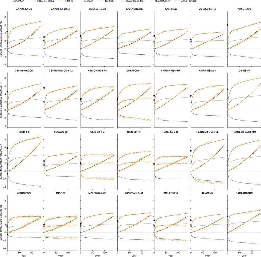
N. J. Leach et al.: FaIRv2.0.0                                                                                                 3011

timescale, but the optimal parameter values are not. Main-         identified for the removal of atmospheric methane – tropo-
taining this timescale at 100 years ensures that the r coeffi-     spheric OH, tropospheric Cl, stratospheric reactions, and soil
cients found here are comparable to the previous iterations of     uptake (Prather et al., 2012; Holmes et al., 2013) – these can
FaIR (Smith et al., 2018; Millar et al., 2017). In the follow-     be aggregated into a single effective atmospheric lifetime.
ing section, we discuss how we parameterize the gas cycle          Through rT and ra , we include the key lifetime feedback de-
to enable FaIRv2.0.0 to simulate a wide range of GHGs us-          pendence on to its own atmospheric burden and tropospheric
ing these same three equations. Qualitative analogies for each     air temperature and water vapour mixing ratio (Holmes et al.,
parameter are given in Table 1 to aid understanding.               2013). We tune ra to match the sensitivity of the methane life-
   Here we emphasize the advantage of using this com-              time to its own atmospheric burden at the present-day found
mon framework to simulate the response to all the differ-          by Holmes et al. (2013). rT is tuned to match the sensitiv-
ent GHG and aerosol emissions: if a user is able to under-         ity of the methane lifetime to tropospheric air temperature
stand the FaIRv2.0.0 carbon cycle, then they understand how        and water vapour at the present-day found by Holmes et al.
the model will respond to emissions of any other GHG or            (2013). Since both tropospheric air temperature and water
aerosol. This is because carbon dioxide is the most com-           vapour are closely related to surface air temperatures (they
plex parameterization of the above equations: being the only       are often approximated by simple parameterizations of the
species with more than one atmospheric decay timescale, and        surface air temperature, as in Holmes et al., 2013), including
alongside methane it is one of only two species to make use        these two sensitivities through a single surface temperature
of the state dependence through α within the default param-        feedback closely replicates lifetime behaviour if both are in-
eterization. This structural simplicity makes gaining famil-       cluded separately. See Fig. S2 in the Supplement for the evo-
iarity with the model far easier than if several different gas     lution of the methane lifetime within default FaIRv2.0.0 over
cycle formulations were used for different GHGs.                   history and a future RCP8.5 pathway (Riahi et al., 2011). τ is
                                                                   then set such that the mean emission rate since 2000 matches
2.1.1   Parameterizing the gas cycle for a wide range of           current estimates from the RCMIP protocol (Nicholls et al.,
        GHGs                                                       2020a; Nicholls and Lewis, 2021) when historical concentra-
                                                                   tions (Meinshausen et al., 2017) are inverted by FaIRv2.0.0,
In this section, we consider how these equations can be pa-        and r0 is set such that α = 1 at model initialization. The pre-
rameterized to represent the gas cycles for many different         industrial concentration is fixed at 720 ppb.
GHGs. We also provide default parameterizations for each
GHG, given in full in Table S2 in the Supplement.
                                                                   Nitrous oxide
Carbon dioxide
                                                                   Nitrous oxide is parameterized with a single atmospheric
As discussed above in Sect. 2.1, FaIRv2.0.0 retains the state-     sink and no lifetime sensitivities: n = 1 and {ru , rT , ra } = 0.
dependent formulation (Millar et al., 2017) of the four-           Although there is evidence that nitrous oxide has a small sen-
timescale impulse response model from Joos et al. (2013);          sitivity to its atmospheric burden (Prather et al., 2015), when
hence, n = 4. We retain the same state dependency as in Mil-       included in FaIRv2.0.0 this made very little difference to ni-
lar et al. (2017), and thus the r parameters are non-zero with     trous oxide concentrations, even under high-emission scenar-
the exception of ra . The default a and τ coefficients are the     ios. We therefore do not include this additional complexity. τ
multi-model mean from Joos et al. (2013). Default ru and           is tuned to match the cumulative RCMIP protocol emissions
rT parameters are taken as the mean of the parameter dis-          when historical concentrations are inverted by FaIRv2.0.0,
tributions inferred from CMIP6 models in Sect. 4.2.1. Fol-         and r0 is set such that α = 1 at model initialization. The pre-
lowing Jenkins et al. (2018), we tune the default r0 parame-       industrial concentration is fixed at 270 ppm.
ter such that present-day (2018) cumulative CO2 emissions
match the RCMIP emission protocol (Nicholls et al., 2020a;
                                                                   Halogenated gases
Nicholls and Lewis, 2021) when historical concentrations
(Meinshausen et al., 2017) are inverted back to emissions by
Eqs. (2)–(4). Here we take the RCMIP protocol as one esti-         All other GHGs are treated as having a single atmospheric
mate of observed emissions, but it is important to note that       lifetime and no feedbacks: n = 1 and {ru , rT , ra } = 0. We
using a different dataset such as the Global Carbon Project        take lifetime estimates from WMO (2018). Pre-industrial
(Friedlingstein et al., 2019) would result in a different value.   concentrations (if non-zero) are set to the 1750 CE value
The pre-industrial concentration is fixed at 278 ppm.              from Meinshausen et al. (2017). Inclusion of a temperature-
                                                                   dependent lifetime to represent changes to the Brewer–
Methane                                                            Dobson circulation (Butchart and Scaife, 2001), as in the
                                                                   MAGICC SCM (Meinshausen et al., 2011a), would be pos-
We parameterize methane using a single atmospheric sink:           sible through a non-zero rT parameter. We do not include
n = 1. Although several individual mechanisms have been            a representation of this effect in our default parameteriza-

https://doi.org/10.5194/gmd-14-3007-2021                                              Geosci. Model Dev., 14, 3007–3036, 2021
3012                                                                                                    N. J. Leach et al.: FaIRv2.0.0

Table 1. Qualitative analogies for named parameters in FaIRv2.0.0.

  Parameter      Units                            Qualitative description
  E(t)           see Table S1 in the Supplement   Quantity of agent emitted into atmosphere
  C(t)           see Table S1                     Concentration of agent in atmosphere
  C0             unit(C)                          Pre-industrial concentration of agent in atmosphere
  Ri (t)         unit(E)                          Quantity of agent in ith atmospheric pool
  ai             –                                Fraction of emissions entering ith atmospheric pool
  τi             years                            Atmospheric lifetime of gas in ith pool
  α(t)           –                                Multiplicative adjustment coefficient of pool lifetimes
  r0             –                                Strength of pre-industrial uptake from atmosphere
  ru             unit(E)−1                        Sensitivity of uptake from atmosphere to cumulative uptake of agent since model ini-
                                                  tialization
  rT             K−1                              Sensitivity of uptake from atmosphere to model temperature change since initialization
  ra             unit(E)−1                        Sensitivity of uptake from atmosphere to current atmospheric burden of agent
  Gu (t)         unit(E)                          Cumulative uptake of agent since model initialization
  T              K                                Model temperature change since initialization
  Ga (t)         unit(E)                          Atmospheric burden of agent above pre-industrial levels
  F (t)          W m−2                            Effective radiative forcing change since the pre-industrial period
  f1             W m−2                            Logarithmic concentration–forcing coefficient
  f2             W m−2 unit(C)−1                  Linear concentration–forcing coefficient
  f3             W m−2 unit(C)−1/2                Square root concentration–forcing coefficient
  Sj (t)         K                                Response of j th thermal box
  qj             K W−1 m2                         Equilibrium response of j th thermal box
  dj             years                            Response timescale of j th thermal box
  T (t)          K                                Surface temperature response since model initialization

tion due to its small impact on model output and increase in            the Brewer–Dobson circulation which modulate the lifetimes
model complexity.                                                       of these gases (Meinshausen et al., 2011a). We note that
                                                                        for these gases we could have matched historical concentra-
Aerosols                                                                tions closer by tuning the lifetimes to the RCMIP protocol
                                                                        data and historical concentration time series (Nicholls et al.,
Aerosols have considerably shorter lifetimes than the                   2020a; Meinshausen et al., 2017) but argue that taking the
timescales generally considered by SCMs (Kristiansen et al.,            best-estimate lifetimes from WMO (2018) is defensible: it
2016). In FaIRv2.0.0, as in previous iterations (Smith et al.,          is more transparent and avoids source-dependent parameters
2018) and other SCMs (Meinshausen et al., 2011a), they are              (if a different emission dataset were used, the resulting tuned
therefore converted directly from emissions to radiative forc-          lifetimes would be different). The lower CO2 concentration
ing. In FaIRv2.0.0, this can be achieved by setting n = 1,              projections in FaIRv2.0.0 compared to FaIRv1.5 are due to
τ = 1, and providing a unit conversion factor of 1 between              weaker temperature and cumulative carbon uptake feedbacks
emissions and “concentrations”.                                         (lower ru and rT ) as inferred from the CMIP6 carbon cycle
2.1.2      Historical and SSP concentration trajectories                tunings performed in Sect. 3.2.

Here we compare the default parameterization gas cycle                  Specification of natural emissions
model in FaIRv2.0.0-alpha to a previous version, FaIRv1.5
(Smith et al., 2018), and to MAGICC7.1.0-beta (Mein-                    In FaIRv2.0.0 we have chosen to formulate the gas cycle
shausen et al., 2020), highlighting any differences. All                equations in terms of a perturbation above the pre-industrial
three models are run under the fully emission-driven “esm-              (natural equilibrium) concentration. By definition, this as-
allGHG” RCMIP protocol (Nicholls et al., 2020a; Nicholls                sumes a time-independent quantity of natural emissions for
and Lewis, 2021). FaIRv2.0.0 matches trajectories from both             each gas (which can be derived from the pre-industrial con-
its previous iteration and the more comprehensive MAG-                  centration and lifetime of the gas). This differs from Mein-
ICC closely for all GHGs. We note some discrepancies in                 shausen et al. (2011a) and Smith et al. (2018), who (when
the time series for halogenated gases between FaIRv2.0.0                driving the respective models with emissions and with the ex-
and MAGICC, possibly due to the incorporation of a state-               ception of CO2 ) require a quantity of natural emissions to be
dependent OH abundance and representation of changes to                 supplied in addition to any anthropogenic emissions by de-

Geosci. Model Dev., 14, 3007–3036, 2021                                                  https://doi.org/10.5194/gmd-14-3007-2021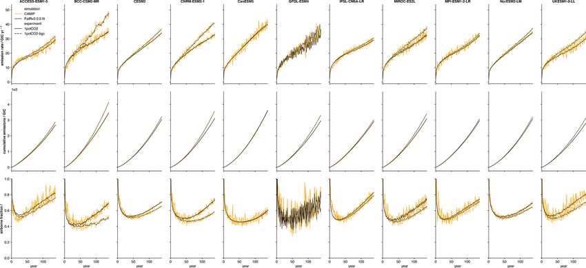
N. J. Leach et al.: FaIRv2.0.0                                                                                                              3013

fault (though the models can also be run in a fully emission-                    2.2.1   Parameterizing the forcing equation
driven mode as in Fig. 2). Over the historical period, these
emissions are chosen such that they “close the budget” be-                       Carbon dioxide, nitrous oxide, and methane
tween total anthropogenic emissions and observed concen-
trations (Meinshausen et al., 2011a; Smith et al., 2018). This                   We assume the forcing relationship for carbon dioxide is
procedure of balancing the budget over history is analogous                      well approximated by the combination of a logarithmic and
to driving the model with concentrations up to the present                       square-root term (Ramaswamy et al., 2001), f2CO2 = 0; both
day and then switching to driving the model with emissions                       the methane and nitrous oxide concentration–forcing re-
afterwards. While this methodology has the advantage of en-                      lationships are approximated by a square-root term only:
                                                                                   CH4 ,N2 O
suring the model simulates present-day concentrations that                       f1,2        = 0. Although overlaps between the spectral bands
match observation exactly, it loses consistency between the                      of these gases mean more complex function forms including
way in which the model simulates the past and the future.                        interaction terms represent our current best approximation to
If care is not taken when running these models, this loss of                     the observed relationship from spectral calculation (Etminan
consistency could lead to discontinuities at the present day                     et al., 2016), inclusion of these interaction terms significantly
(when the model switches from concentration- to emission-                        increases the structural complexity of the model. These over-
driven). As present-day trends are crucial for the estimation                    lap terms are most significant for very high concentrations
of many policy and scientifically relevant quantities such as                    of these gases, and we find that the more simple relation-
TCR, TCRE, and remaining carbon budgets (Leach et al.,                           ships used here are sufficiently accurate within the context
2018; Tokarska et al., 2020; Jiménez-de-la Cuesta and Mau-                       of the uncertainties associated with such high-concentration
ritsen, 2019), we have chosen to enforce a consistent model                      scenarios. We fit the non-zero f coefficients to the Oslo-line-
(i.e. emission-driven or concentration-driven) over the entire                   by-line (OLBL) data from Etminan et al. (2016). Our result-
simulation period in FaIRv2.0.0. We note that replicating this                   ing fits have a maximum absolute error of 0.115 W m−2 when
budget closing procedure is possible in FaIRv2.0.0 by invert-                    compared to the OLBL data, though this is for the most ex-
ing observed concentrations to emissions and then joining                        treme high-concentration data point, and the associated rel-
these inverse emission time series to any future scenarios                       ative error is 1.1 %. Figure S1 in the Supplement provides a
manually. In this study, FaIRv2.0.0 is run in emission-driven                    complete comparison of how the fit relationships used here
mode unless stated otherwise.                                                    compare to the OLBL data and the simple formulae that in-
                                                                                 clude interaction terms in Etminan et al. (2016).

2.2   Effective radiative forcing                                                Halogenated GHGs

                                                                                 Following other simple models (Smith et al., 2018; Mein-
FaIRv2.0.0 uses a simple formula to relate atmospheric                           shausen et al., 2011a), we assume concentrations of halo-
gas concentrations to effective radiative forcing. This equa-                    genated gases are linearly related to their direct effective ra-
tion, Eq. (6), includes logarithmic, square-root, and linear                                       x = 0. The conversion coefficient for each
                                                                                 diative forcing, f1,3
terms, motivated by the concentration–forcing relationships                      gas is its radiative efficiency, which we take from WMO
in Myhre et al. (2013) of CO2 , CH4 and N2 O, and all                            (2018).
other well-mixed GHGs (WMGHGs), respectively. For most
agents, the concentration–forcing (or for aerosols, emission–                    Aerosol–radiation interaction
forcing) relationship can be reasonably approximated by one
of these terms in isolation, however if there is substantial ev-                 We follow Smith et al. (2020), parameterizing the ERF due
idence the relationship deviates significantly from any one                      to aerosol radiation interaction as a linear function of sulfate,
term, others are able to be included to provide a more accu-                     organic carbon, and black carbon aerosol emissions:
rate fit. Fext is the sum of all exogenous forcings supplied.
These may include natural forcing agents or forcing due to
albedo changes.                                                                  ERFari = f2SO2 E SO2 + f2OC E OC + f2BC E BC .               (7)

                                                                                 Default parameters are taken as the central estimate from the
                                                                                 “constrained” ensemble described in Sect. 4.
          forcing
               Xagents               C x (t)

F (t) =                    f1x   · ln           + f2x · [C x (t) − C0x ]         Aerosol–cloud interaction
               x                       C0x
                                                                           (6)   ERF due to aerosol–cloud interactions is parameterized fol-
                    hp             q     i                                      lowing a modification of Smith et al. (2020), as a logarithmic
          + f3x ·        C x (t) − C0x        + Fext
                                                                                 function of sulfate aerosol emissions and a linear function of

https://doi.org/10.5194/gmd-14-3007-2021                                                           Geosci. Model Dev., 14, 3007–3036, 2021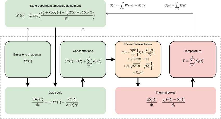
3014                                                                                                    N. J. Leach et al.: FaIRv2.0.0

Figure 2. Comparison of historical and future concentration trajectories over a range of SSPs. Values for all GHGs are in parts per billion
with the exception of CO2 , which is plotted in parts per million. Inset panels for CO2 , CH4 , and N2 O show the historic period.

organic carbon and black carbon aerosol emissions:                      Sect. 3.3. Default parameters are taken as the central estimate
                                                                        from the constrained ensemble described in Sect. 4.
                                 !
                         E SO2
ERFaci = f1aci ln   1+               + f2aci (E OC + E BC ).   (8)      Ozone
                         C0SO2
                                                                        Ozone is parameterized following Thornhill et al. (2021),
Here C0SO2 effectively acts as a shape parameter for the loga-          as a linear function of methane; nitrous oxide and ozone-
rithmic term. We fit this functional form to the ERFaci com-            depleting substances (ODSs) concentrations; and nitrate
ponent in 10 CMIP6 models derived by the approximate par-               aerosol, carbon monoxide, and volatile organic compound
tial radiative perturbation method (Zelinka et al., 2014) in            emissions. This parameterization is tuned such that the over-

Geosci. Model Dev., 14, 3007–3036, 2021                                                  https://doi.org/10.5194/gmd-14-3007-2021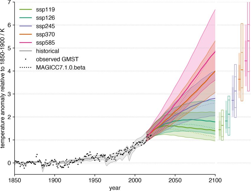
N. J. Leach et al.: FaIRv2.0.0 3015
all ozone forcing time series reproduces Skeie et al. (2020). 2.4 Temperature response
The contribution of individual ODSs to their total is based
on their estimated equivalent effective stratospheric chlo- The final component of the model calculates the surface tem-
rine (Newman et al., 2007; Velders and Daniel, 2014; Smith perature response to the changes in ERF. A common repre-
et al., 2018), with fractional release factors from Engel et al. sentation of this physical process is the energy balance model
(2018). outlined by Geoffroy et al. (2013). Here we consider the
three-box energy balance model, including the ocean heat
Stratospheric water vapour uptake efficacy factor introduced by Held et al. (2010). Re-
cent literature has suggested that a two-box energy balance
model is insufficient to capture the full range of behaviour
Stratospheric water vapour is assumed to be a linear func-
observed in CMIP6 models (Tsutsui, 2020, 2017; Cummins
tion of methane concentrations (Smith et al., 2018) due to its
et al., 2020). The three-box model can be written in state
small magnitude. The default coefficient is derived from the
space form as follows:
5th Assessment Report forcing estimate (Myhre et al., 2013)
and historical methane concentrations (Meinshausen et al., Ẋ(t) = AX(t) + bF (t), (9)
2017): 4.37 × 10⁻⁵ W m−2 ppb−1 . T
where X(t) = T1 (t) T2 (t) T3 (t) ,
Black carbon on snow −(λ + κ2 )/C1 κ2 /C1 0
A = κ2 /C2 −(κ2 + κ3 )/C2 κ3 /C2 ,
0 κ3 /C3 −κ3 /C3
ERF due to light-absorbing particles on snow and ice remains T
a linear function of black carbon emissions (Smith et al., and b = 1/C1 0 0 .
2018). In AR5, the best estimate of its associated ERF was
0.04 W m−2 (Myhre et al., 2013). However, this value is very Here, each box i has a temperature Ti and heat capacity Ci .
uncertain, and the efficacy of black carbon on snow may at F is the prescribed radiative forcing. Heat exchange coeffi-
least double this value (Bond et al., 2013). We therefore cal- cients κ represent the strength of thermal coupling between
culate our default forcing efficiency by dividing an adopted boxes i and i − 1. λ is the so-called climate feedback pa-
value of −0.08 W m−2 by the RCMIP protocol emission rate: rameter. is the efficacy factor that enables the energy bal-
0.0116 W m−2 MtBC−1 . ance model to account for the variations in λ during periods
of transient warming observed in general circulation models
(GCMs). T1 represents the surface temperature change rela-
Contrails tive to a pre-industrial climate. For many users of SCMs, the
key variable of interest is T1 , i.e. the surface temperature re-
Combined ERF due to contrails and contrail-induced cir- sponse. To allow parameters of this energy balance model to
rus is modelled as a linear function of aviation sec- be fit to finite-length CMIP6 experiments with any degree of
tor NOx emissions. The default coefficient is calculated certainty, Cummins et al. (2020) also take advantage of the
by dividing the best-estimate present-day contrail ERF following relationship with the top of atmosphere flux, N (t):
(Lee et al., 2021) by the RCMIP protocol emission rate:
0.0164 W m−2 MtNOx −1 . N (t) = F (t) − λT1 (t) + (1 − )κ3 [T2 (t) − T3 (t)]. (10)
Albedo shift due to land use change
However, calculating the surface temperature response to ra-
diative forcing within the energy balance model can be sim-
In this study we prescribe ERF due to land use change exter- plified by diagonalizing Eq. (9), resulting in an impulse re-
nally. However, it could be incorporated in a manner identical sponse in T1 (henceforth referred to as T ), giving the thermal
to FaIRv1.5 by supplying a time series of cumulative land use response form in Millar et al. (2017) (Tsutsui, 2017):
change CO2 emissions and scaling linearly by a coefficient of
−0.00114 W m−2 GtC−1 (Smith et al., 2018). dSj (t) qj F (t) − Sj (t)
= , (11)
dt dj
2.3 Default parameter metric values for comparison 3
X
and T (t) = Sj (t). (12)
Table S3 in the Supplement contains default parameter cal- j =1
culated values for the global warming potential (Lashof
and Ahuja, 1990) of each emission type simulated in We can relate the energy balance model matrix representa-
FaIRv2.0.0. These values are intended to aid comparison be- tion to the impulse response parameters as follows. If we let
tween FaIRv2.0.0 and other SCMs and do not represent any 8 be the matrix that diagonalizes A such that 8−1 A8 = D,
new analysis. where D is a diagonal matrix with the eigenvalues of A on
https://doi.org/10.5194/gmd-14-3007-2021 Geosci. Model Dev., 14, 3007–3036, 20213016 N. J. Leach et al.: FaIRv2.0.0
the diagonals, then the response timescales are di = −1/Dii surface temperature response from ESGF (Cinquini et al.,
(Geoffroy et al., 2013). The response coefficients are qi = 2014). These data are normalized as described in Nicholls
di 8−1
i,0 80,i /C1 . In FaIRv2.0.0, we use this three-timescale et al. (2021). To reduce internal variability in the input time
impulse response form due to its simplicity and flexibility. series used to fit parameters, we average over all available
Two common measures of the climate sensitivity, the equilib- ensemble members for each model. The number of ensem-
rium climate sensitivity (ECS) and transient climate response ble members per model is stated in Table S4 in the Supple-
(TCR) (Collins et al., 2013) are easily expressed in terms of ment. The Cummins et al. (2020) methodology uses surface
the impulse response parameters: temperatures and top-of-atmosphere energy imbalances (as
related by Eq. 10) from the abrupt-4xCO2 experiment to re-
3
X turn all the parameters of the energy balance model, plus
ECS = F2×CO2 · qj , (13)
j =1
the radiative forcing arising from the quadrupling of carbon
dioxide concentrations. While this would fully specify both
3
X dj − d70 the thermal response and the concentration–forcing relation-
TCR = F2×CO2 · qj 1− 1−e j . (14)
j =1
70 ship if concentration–forcing was a pure logarithmic rela-
tionship, several models display significant deviations from
The default thermal response parameters in FaIRv2.0.0 are a pure logarithmic concentration–forcing relationship (Tsut-
derived as follows: d1 = 0.903, d2 = 7.92, d3 = 355, and sui, 2020, 2017). We account for this within the FaIRv2.0.0
q1 = 0.180 are taken as their central value within the con- framework by assuming that the concentration–forcing re-
strained ensemble in Sect. 4.3, which do not differ sig- lationship can be reasonably approximated by the sum of
nificantly from the CMIP6 inferred distribution described a logarithmic and square-root term. Best-estimate f1CO2 and
in Sect. 4.2.3. q2 = 0.297 and q3 = 0.386 are then set by f3CO2 parameters are found by first deriving the TCR of each
Eqs. (13) and (14) such that the default parameter set re- model using the 1pctCO2 experiment. We can use the tuned
sponse has climate sensitivities (ECS and TCR) equal to impulse response parameters and TCR to then calculate the
the central values of the constrained ensemble described in forcing at a doubling of carbon dioxide using the relation-
Sect. 4: ECS = 3.24 K and TCR = 1.79 K. ship in Eq. (14). The forcings at carbon dioxide doubling and
quadrupling uniquely specify f1CO2 and f3CO2 values for use
3 Emulating complex climate models in FaIRv2.0.0. The best-estimate impulse response and f pa-
rameters, climate sensitivities, and forcings at carbon dioxide
In this section we demonstrate the ability of FaIRv2.0.0 doubling and quadrupling are given in Table 2. Correspond-
to emulate the more complex models from CMIP6 (Eyring ing energy balance model parameters are given in Table S5.
et al., 2016) in a limited set of experiments. Due to con- Figure 3 shows the emulated and original responses to the
straints on data availability, we have focussed on tuning the abrupt-4xCO2 and 1pctCO2 experiments for each model.
key components of the model: the carbon cycle, the ther-
mal response, and the aerosol ERF relationships. We use the 3.2 Tuning the carbon cycle response
abrupt-4xCO2 and 1pctCO2 CMIP6 experiments to tune the
carbon cycle and thermal response. The highly idealized na- We tune the carbon cycle using CMIP6 data from the C4MIP
ture of these experiments means that parameters arising from (Jones et al., 2016) fully coupled and biogeochemically cou-
these tunings will not necessarily be able to emulate complex pled 1pctCO2 runs (Arora et al., 2020). Since constraining
model response to more realistic scenarios due to processes the response coefficients ai and timescales τi requires pulse
that FaIRv2.0.0 cannot represent. In the near future we hope emission experiments such as those carried out by Joos et al.
to be able to tune to the historical and SSP CMIP6 experi- (2013), here we only fit the r feedback parameters and keep
ments in order to validate the tunings given here. the response coefficients, a, and timescales, τ , equal to the
multi-model mean from Joos et al. (2013). The inclusion of
3.1 Tuning the thermal response both the fully coupled and biogeochemically coupled runs in
the procedure allows us to constrain ru , ra , and rT indepen-
We follow the statistically rigorous methodology of Cum- dently. We use Eqs. (2) and (3) to diagnose the values of α
mins et al. (2020) to tune thermal response parameters to 28 required to reproduce the C4MIP emissions from the corre-
CMIP6 models. This involves fitting parameters to the en- sponding concentrations within the FaIRv2.0.0 carbon cycle
ergy balance model outlined in Eq. (9) by recursively com- impulse response framework. We then use Eq. (4) to con-
puting the likelihood via a Kalman filter; the optimal param- vert α into iIRF100 time series. Finally, we use an ordinary
eters are those that maximize the computed likelihood. We least-squares estimator to calculate r parameters by regress-
then transform the optimal energy balance parameters into ing the C4MIP cumulative uptake, temperature, and atmo-
the impulse response form used in FaIRv2.0.0. We obtain spheric burden time series against the diagnosed iIRF100 time
model data from the “abrupt-4xCO2”, “1pctCO2” and “pi- series. r0 is taken as the intercept of the estimator. We include
Control” experiments for the top-of-energy imbalance and the atmospheric burden as a predictor (and hence obtain non-
Geosci. Model Dev., 14, 3007–3036, 2021 https://doi.org/10.5194/gmd-14-3007-2021N. J. Leach et al.: FaIRv2.0.0 3017
Table 2. Tuned CMIP6 thermal response parameters.
Parameter
Model d1 d2 d3 q1 q2 q3 f1 f2 f3 ECS TCR F2×CO2 F4×CO2
ACCESS-CM2 0.635 7.76 319 0.131 0.495 0.794 −0.799 0 0.515 4.32 1.98 3.04 7.58
ACCESS-ESM1-5 2.34 66.6 1 040 000 000 0.445 0.426 2.45 × 10⁻⁶ 4.83 0 0.00086 2.92 1.99 3.35 6.71
AWI-CM-1-1-MR 1.09 6.29 163 0.203 0.306 0.335 4.3 0 0.117 3.2 2.05 3.79 7.93
BCC-CSM2-MR 0.976 5.78 208 0.192 0.23 0.402 0.821 0 0.408 2.82 1.58 3.42 8.02
BCC-ESM1 2.21 15.2 353 0.373 0.328 0.519 2.07 0 0.171 3.21 1.76 2.63 5.76
CAMS-CSM1-0 0.577 4.92 135 0.0991 0.284 0.154 6.26 0 0.00235 2.34 1.73 4.36 8.72
CESM2-FV2 0.531 4.37 417 0.0862 0.448 1.26 2.0 0 0.278 5.97 2.01 3.32 7.45
CESM2-WACCM 0.328 4.88 326 0.0516 0.482 0.864 0.0334 0 0.468 4.6 1.93 3.29 7.94
CESM2-WACCM-FV2 0.621 6.51 458 0.132 0.485 1.16 3.17 0 0.132 5.54 2.04 3.12 6.62
CMCC-CM2-SR5 1.54 29.3 567 000 0.337 0.368 0.00106 3.83 0 0.178 2.75 2.17 3.89 8.3
CNRM-CM6-1 1.8 24.7 754 0.324 0.442 5.81 × 10⁻⁶ 0.591 0 0.465 2.8 2.23 3.66 8.66
CNRM-CM6-1-HR 1.72 15.6 296 0.265 0.445 0.19 4.61 0 0.11 3.57 2.48 3.97 8.25
CNRM-ESM2-1 0.914 8.27 317 0.133 0.694 0.724 −1.04 0 0.429 3.53 1.86 2.28 5.79
CanESM5 1.22 11.1 289 0.227 0.602 0.779 2.06 0 0.257 5.18 2.63 3.22 7.19
E3SM-1-0 0.973 11.0 272 0.202 0.673 0.847 3.7 0 0.117 5.83 2.94 3.39 7.11
FGOALS-g3 0.88 5.03 240 0.15 0.307 0.34 0.403 0 0.422 2.57 1.54 3.23 7.67
GISS-E2-1-G 0.528 5.24 713 0.223 0.222 0.0535 2.44 0 0.341 2.03 1.75 4.07 9.12
GISS-E2-1-H 1.49 31.2 24 900 000 0.33 0.311 0.0343 4.23 0 0.107 2.49 1.88 3.68 7.67
GISS-E2-2-G 0.872 10.7 514 0.198 0.229 0.0114 7.3 0 −0.0931 1.94 1.72 4.41 8.55
HadGEM3-GC31-LL 0.756 8.59 269 0.143 0.592 0.851 1.2 0 0.343 5.13 2.46 3.23 7.45
HadGEM3-GC31-MM 1.01 11.2 244 0.209 0.51 0.731 3.81 0 0.136 5.21 2.62 3.59 7.58
MIROC-ES2L 0.935 12.8 3400 0.199 0.232 7.18 × 10⁻⁶ 0.351 0 0.526 1.68 1.51 3.91 9.34
MIROC6 1.13 47.6 94 700 000 0.302 0.155 0.0037 3.76 0 0.231 1.94 1.56 4.22 9.1
MPI-ESM1-2-HR 2.16 54.0 842 000 000 0.344 0.237 3.37 × 10⁻⁶ 1.71 0 0.37 2.19 1.65 3.76 8.6
MPI-ESM1-2-LR 1.18 6.15 256 0.156 0.244 0.237 3.33 0 0.316 2.87 1.83 4.51 9.94
MRI-ESM2-0 0.917 7.13 254 0.197 0.404 0.558 2.2 0 0.161 3.07 1.66 2.65 5.76
NorCPM1 1.47 7.1 282 0.172 0.254 0.457 2.41 0 0.264 3.1 1.58 3.52 7.79
SAM0-UNICON 0.828 4.61 298 0.106 0.408 0.453 6.42 0 −0.0386 4.05 2.24 4.18 8.26
zero ra values) due to a significant reduction in regression Table 3. Tuned CMIP6 carbon cycle parameters.
residual for several models when included. We find that all
the C4MIP models display an exceptionally high, rapidly de- Parameter
creasing initial airborne fraction. In terms of the FaIRv2.0.0 Model r0 ru rT ra
equations, this corresponds to an α value that decreases ini-
ACCESS-ESM1-5 36.7 0.035 3.04 −0.00066
tially before reaching a minimum, representing a carbon sink
BCC-CSM2-MR 25.6 0.00598 5.2 0.00439
that initially increases in strength when concentrations start CESM2 40.7 0.0107 1.28 0.00421
to rise before decreasing as the concentrations and tempera- CNRM-ESM2-1 38.1 0.000581 2.47 0.00978
tures rise further. FaIRv2.0.0 is unable to fully capture this CanESM5 35.7 −0.00596 −0.104 0.0181
initial adjustment, and as such in our tunings we prioritize GFDL-ESM4 34.3 0.0219 4.86 −0.00424
emulating the long-term behaviour and carry out the regres- IPSL-CM6A-LR 32.2 0.0166 1.07 0.0123
sion from year 60 onwards. It would be possible to better MIROC-ES2 L 33.4 0.0131 3.46 0.00399
MPI-ESM1-2-LR 33.3 0.031 1.5 −0.00257
capture the initial adjustment by including additional terms
NorESM2-LM 40.7 0.00947 1.56 0.00489
in Eq. (4), but since it remains to be seen whether this be- UKESM1-0-LL 37.9 0.0201 2.67 0.00181
haviour is apparent in scenarios where concentrations do not
rise suddenly and rapidly from a pre-industrial level as is the
case in the 1pctCO2 experiment (such as a historical emission
scenario), we do not do so here. Tuned parameters are given 3.3 Tuning aerosol ERF
in Table 3, with Fig. 4 showing diagnosed C4MIP emissions
and the FaIRv2.0.0-alpha emulation. We note that these tun- Aerosol forcing relationships are tuned to ERF data from 10
ings suggest that the pre-industrial sink strength (which is CMIP6 models and emission data from the RCMIP protocol
encapsulated by r0 ) in 7 out of 11 models is higher than the (Nicholls et al., 2020a; Nicholls and Lewis, 2021) follow-
historically observed best estimate found here (Sect. 2.1.1) ing Smith et al. (2020). For each CMIP6 model, aerosol–
and in a previous study (Jenkins et al., 2018). radiation and aerosol–cloud interaction components of the
ERF are calculated by the approximate partial radiative per-
turbation (APRP) method. For additional details on the exact
procedure, see Smith et al. (2020) and Zelinka et al. (2014).
https://doi.org/10.5194/gmd-14-3007-2021 Geosci. Model Dev., 14, 3007–3036, 20213018 N. J. Leach et al.: FaIRv2.0.0 Figure 3. FaIRv2.0.0 emulation of CMIP6 model response to the abrupt-4xCO2, abrupt-2xCO2, abrupt-0p5xCO2, and 1pctCO2 experiments. The black line shows FaIRv2.0.0-alpha emulation, and the orange line shows CMIP6 model data where available. Emulation parameters were fit using the abrupt-4xCO2 and 1pctCO2 experiments so the abrupt-2xCO2 and abrupt-0p5xCO2 simulations can be considered as verification experiments for the models where the data for these experiments is available. Filled and unfilled dots over the y axis indicate the assessed model ECS and TCR, respectively (see Table 2). For each model, we fit the f coefficients in Eq. (7) to the 1965). The tuned parameters are given in Table 4. Figure 5, ERFari component using an ordinary least-squares estimator. following Fig. 2 of Smith et al. (2020), shows the parameter- The resulting coefficients are almost identical to those from ized fits compared to the APRP-derived model ERF compo- Smith et al. (2020), with differences arising only due to the nents. emission data used. We then fit the f coefficients and C0SO2 in Eq. (8) to the ERFaci component by minimizing the residual sum of squares using a simplex algorithm (Nelder and Mead, Geosci. Model Dev., 14, 3007–3036, 2021 https://doi.org/10.5194/gmd-14-3007-2021
N. J. Leach et al.: FaIRv2.0.0 3019
Figure 4. FaIRv2.0.0 emulation of CMIP6 model carbon cycle response to the C4MIP 1pctCO2 experiments. The black line shows
FaIRv2.0.0-alpha emulation, and the orange line shows C4MIP model data. The top row shows diagnosed emission rates, the middle row
shows cumulative emissions, and the bottom row shows airborne fraction. The solid line indicates the fully coupled C4MIP runs, while the
dashed lines show biogeochemically coupled runs (emulated in FaIRv2.0.0-alpha by setting rT = 0).
Table 4. Tuned CMIP6 aerosol forcing parameters.
Source ERFari ERFaci
SO2 SO2
Parameter f2 f2BC f2OC f1aci C0 f2aci
Model
CanESM5 −0.00249 0.0326 −0.000347 −0.387 23.8 −0.0152
E3SM −0.000942 0.0248 −0.0126 −1.64 113 −0.0142
GFDL-CM4 −0.00261 0.0269 −0.00209 −2.23 427 −0.00803
GFDL-ESM4 −0.00264 0.102 −0.0304 −57.6 17000 −0.0153
GISS-E2-1-G −0.00668 0.146 −0.0441 −0.156 16.8 −0.0176
HadGEM3-GC31-LL −0.00291 0.00196 0.00415 −0.783 66.9 −0.00691
IPSL-CM6A-LR −0.000748 −0.0561 0.00885 −0.951 306 −0.00173
MIROC6 −0.00178 0.0387 −0.0142 −0.392 46.6 −0.0124
NorESM2-LM −0.00126 0.00302 −0.0034 −68.6 10300 −0.0123
UKESM1-0-LL −0.00239 0.00255 6.32 × 10⁻⁵ −0.74 38.9 −0.000265
4 Constraining probabilistic parameter ensembles 4.1 The current level and rate of warming
The computational efficiency of SCMs makes them an ideal We determine the current level and rate of warming fol-
tool for carrying out large ensemble simulations from which lowing the Global Warming Index methodology (Haustein
probabilistic projections can be derived. Smith et al. (2018) et al., 2017). This takes into account multiple sources of
carried out such a large ensemble and produced projections uncertainty: observational, forcing, Earth system response
based on constraining the ensemble members to fall within (through parameter variation in an identical climate response
the 5 %–95 % uncertainty range in observed warming to date model to the one used in FaIRv2.0.0), and internal variability.
from the Cowtan and Way dataset (Cowtan and Way, 2014). With this methodology, we obtain an estimate of the distribu-
Here we replicate this procedure with the new model but us- tion of the current (2010–2019) level and rate of the anthro-
ing a new constraint methodology and updated prior param- pogenic contribution to global warming (the anthropogenic
eters distributions. warming index distribution). A key choice within this esti-
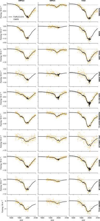
https://doi.org/10.5194/gmd-14-3007-2021 Geosci. Model Dev., 14, 3007–3036, 20213020 N. J. Leach et al.: FaIRv2.0.0 Figure 5. FaIRv2.0.0 emulation of CMIP6 model aerosol forcing. The black line shows FaIRv2.0.0-alpha emulation, and the orange dots show CMIP6 model data. All series displayed are relative to zero effective radiative forcing in 1850. Geosci. Model Dev., 14, 3007–3036, 2021 https://doi.org/10.5194/gmd-14-3007-2021
N. J. Leach et al.: FaIRv2.0.0                                                                                                    3021

mate is the observational data product used. There are six            Table 5. Carbon cycle parameter sampling.
widely used products available (Lenssen et al., 2019; Cowtan
and Way, 2014; Vose et al., 2012; Morice et al., 2012, 2020;                  Parameter    default value   scaling factor, X
Rohde et al., 2013). Here we average over the distributions                   r0                    33.9   X ∼ N (1, 0.154)
implied by each product to obtain our final distribution used                 ru                 0.0188    ln(X) ∼ N (0, 0.442)
to constrain our FaIRv2.0.0 ensemble. This choice clearly                     rT                    2.67   X ∼ N (1, 0.615)
projects significantly onto our results, so we provide results
for each dataset in turn in Sect. 4.3.5 to demonstrate the sen-
sitivity of our analysis to the choice of dataset. For full details
                                                                      but exclude the atmospheric burden as a predictor for the
of this calculation, see the Supplement.
                                                                      C4MIP iIRF100 time series. The resulting r0 , ru , and rT pa-
4.1.1    Definition of global mean temperature                        rameter samples are uncorrelated. We sample these param-
                                                                      eters by applying scaling factors inferred from the CMIP6
Recent studies (Richardson et al., 2016, 2018) have shown             tunings to the default parameter values (for ru and rT this is
that the definition of globally averaged surface temperature          equivalent to sampling directly from the distribution inferred
used is important when comparing observations to climate              from the CMIP6 tunings). The underlying uncorrelated scal-
model output, and is relevant when exploring policy-relevant          ing factor distributions are given in Table 5.
quantities such as the carbon budget (Tokarska et al., 2019).
Discrepancies arise since observations blend air temperatures         4.2.2   Forcing parameters
over land and sea ice with water temperature over ocean
                                                                      Uncertainty in effective radiative forcing is included by
and do not have full global coverage (they are blended–
                                                                      grouping individual forcing agents into broader forcing
masked), while climate model surface temperature output is
                                                                      classes (IPCC et al., 2013) and applying a randomly sampled
globally complete and always measured as the air tempera-
                                                                      scaling factor to all the f parameters within each class (with
ture 2 m above the surface of the Earth. It has been shown
                                                                      the exception of aerosol forcings, which we discuss imme-
both historically and over future climate scenarios (Richard-
                                                                      diately below). Scaling factors between forcing classes are
son et al., 2018) that the blended–masked temperature def-
                                                                      uncorrelated. The scaling factor distributions used for each
inition (GMST) may be cooler than the globally complete
                                                                      forcing class are given in Table 6. Uncertainty in aerosol
2 m air temperature definition (GSAT). In our Global Warm-
                                                                      forcing is included as follows. ERFari f coefficients (Eq. 7)
ing Index calculation (Sect. 4.1), we combine six tempera-
                                                                      are first drawn from a multivariate normal distribution in-
ture observation datasets (Lenssen et al., 2019; Cowtan and
                                                                      ferred from the CMIP6 tuned parameters in Table 4. We
Way, 2014; Vose et al., 2012; Morice et al., 2012; Rohde
                                                                      then apply a quantile map to scale the resulting coefficients
et al., 2013; Morice et al., 2020); this implies that our con-
                                                                      such that the 1850 to 2005–2015 mean ERFari distribu-
strained ensemble will broadly measure surface temperatures
                                                                      tion matches the process based assessment in Bellouin et al.
using the GMST definition. This may lead to slightly lower
                                                                      (2020). For ERFaci, f2aci coefficients (Eq. 8) are drawn from
model estimates of surface temperature than if we used the
                                                                      a normal distribution inferred from the CMIP6 tuned param-
GSAT definition. We can estimate the difference between our
                                                                      eters in Table 4. f1aci and C0SO2 coefficients are drawn from a
definition of GMST and GSAT by regressing the six-dataset
                                                                      multivariate log-normal distribution; this ensures we sample
mean used here against GSAT from ERA5 (Hersbach et al.,
                                                                      the full range of ERFaci shapes provided by CMIP6 mod-
2020). A least-squares estimator (confidence calculated us-
                                                                      els. As with the ERFari coefficients, we then apply a quantile
ing a block-bootstrap; Wilks, 1997) suggests that our GMST
                                                                      map to scale these coefficients such that the sampled 1850 to
definition is 4.6 % [0.4 %, 10.8 %] smaller than GSAT2 .
                                                                      2005–2015 mean ERFaci distribution matches Bellouin et al.
4.2     Sampled prior distributions                                   (2020).

4.2.1    Carbon cycle parameters                                      4.2.3   Thermal response parameters

While including the atmospheric burden is necessary to em-            Uncertainty in thermal response is incorporated by sam-
ulate the carbon cycle behaviour of individual C4MIP mod-             pling response parameters directly from distributions in-
els well, parameterizing the iIRF100 as a linear function of          ferred from the CMIP6 tunings in Sect. 2, taking correlations
just cumulative carbon uptake and temperature is sufficient           between parameters into account. Referring to parameters
to capture the spread of the model ensemble. Correlations be-         as in Eqs. (11)–(14), we draw parameters from the follow-
tween parameters also complicate sampling from the inferred           ing distributions. d1 , d2 , and q1 are highly correlated, and
parameter distributions derived from Table 3. We therefore            we therefore sample ln(d1 ), ln(d2 ), and q1 from a multivari-
repeat the parameter tuning procedure described in Sect. 3.2          ate normal distribution with covariances and means taken
                                                                      from the values in Sect. 2. d3 is not strongly correlated with
   2 square brackets indicate a 90 % credible interval                any other parameter, and so we sample ln(d3 ) from a nor-

https://doi.org/10.5194/gmd-14-3007-2021                                                  Geosci. Model Dev., 14, 3007–3036, 2021
You can also read