Temperature controls production but hydrology regulates export of dissolved organic carbon at the catchment scale
←
→
Page content transcription
If your browser does not render page correctly, please read the page content below
Hydrol. Earth Syst. Sci., 24, 945–966, 2020
https://doi.org/10.5194/hess-24-945-2020
© Author(s) 2020. This work is distributed under
the Creative Commons Attribution 4.0 License.

Temperature controls production but hydrology regulates export of
dissolved organic carbon at the catchment scale
Hang Wen1 , Julia Perdrial2 , Benjamin W. Abbott3 , Susana Bernal4 , Rémi Dupas5 , Sarah E. Godsey6 ,
Adrian Harpold7 , Donna Rizzo8 , Kristen Underwood8 , Thomas Adler2 , Gary Sterle7 , and Li Li1
1 Department  of Civil and Environmental Engineering, The Pennsylvania State University, University Park, PA 16802, USA
2 Department  of Geology, University of Vermont, Burlington, VT 05405, USA
3 Department of Plant and Wildlife Sciences, Brigham Young University, Provo, UT 84602, USA
4 Center of Advanced Studies of Blanes (CEAB-CSIC), Accés Cala St. Francesc 14, 17300, Blanes, Girona, Spain
5 INRA, UMR 1069 SAS, Rennes, France
6 Department of Geosciences, Idaho State University, Pocatello, ID 83201, USA
7 Department of Natural Resources and Environmental Science, University of Nevada, Reno, NV 89557, USA
8 Department of Civil and Environmental Engineering, University of Vermont, Burlington, VT 05405, USA

Correspondence: Li Li (lili@engr.psu.edu)

Received: 16 June 2019 – Discussion started: 18 July 2019
Revised: 9 December 2019 – Accepted: 12 January 2020 – Published: 27 February 2020

Abstract. Lateral carbon flux through river networks is an      DOC from the organic-poor groundwater and from organic-
important and poorly understood component of the global         rich soil water in the swales bordering the stream. The DOC
carbon budget. This work investigates how temperature           produced accumulated in hillslopes and was later flushed out
and hydrology control the production and export of dis-         during the wet and cold period (winter and spring) when Re
solved organic carbon (DOC) in the Susquehanna Shale            peaked as the stream reconnected with uphill and Rp reached
Hills Critical Zone Observatory in Pennsylvania, USA. Us-       its minimum.
ing field measurements of daily stream discharge, evapo-           The model reproduced the observed concentration–
transpiration, and stream DOC concentration, we calibrated      discharge (C–Q) relationship characterized by an unusual
the catchment-scale biogeochemical reactive transport model     flushing–dilution pattern with maximum concentrations at
BioRT-Flux-PIHM (Biogeochemical Reactive Transport–             intermediate discharge, indicating three end-members of
Flux–Penn State Integrated Hydrologic Model, BFP), which        source waters. A sensitivity analysis indicated that this non-
met the satisfactory standard of a Nash–Sutcliffe efficiency    linearity was caused by shifts in the relative contribution of
(NSE) value greater than 0.5. We used the calibrated model      different source waters to the stream under different flow
to estimate and compare the daily DOC production rates (Rp ;    conditions. At low discharge, stream water reflected the
the sum of the local DOC production rates in individual grid    chemistry of organic-poor groundwater; at intermediate dis-
cells) and export rate (Re ; the product of the concentration   charge, stream water was dominated by the organic-rich soil
and discharge at the stream outlet, or load).                   water from swales; at high discharge, the stream reflected
   Results showed that daily Rp varied by less than an or-      uphill soil water with an intermediate DOC concentration.
der of magnitude, primarily depending on seasonal temper-       This pattern persisted regardless of the DOC production rate
ature. In contrast, daily Re varied by more than 3 orders of    as long as the contribution of deeper groundwater flow re-
magnitude and was strongly associated with variation in dis-    mained low (< 18 % of the streamflow). When groundwater
charge and hydrological connectivity. In summer, high tem-      flow increased above 18 %, comparable amounts of ground-
perature and evapotranspiration dried and disconnected hill-    water and swale soil water mixed in the stream and masked
slopes from the stream, driving Rp to its maximum but Re        the high DOC concentration from swales. In that case, the C–
to its minimum. During this period, the stream only exported    Q patterns switched to a flushing-only pattern with increasing

Published by Copernicus Publications on behalf of the European Geosciences Union.
946                         H. Wen et al.: The temperature and hydrology control on the production and export of DOC

DOC concentration at high discharge. These results depict         at stream outlets is primarily positive (Moatar et al., 2017;
a conceptual model that the catchment serves as a producer        Zarnetske et al., 2018). Approximately 80 % of watersheds
and storage reservoir for DOC under hot and dry conditions        in the USA and France show a flushing C–Q pattern (i.e.,
and transitions into a DOC exporter under wet and cold con-       the stream DOC concentration increases with discharge),
ditions. This study also illustrates how different controls on    whereas the rest shows dilution (decreasing DOC with dis-
DOC production and export – temperature and hydrological          charge) or chemostatic behavior (negligible concentration
flow paths, respectively – can create temporal asynchrony         change with discharge). These C–Q patterns generally cor-
at the catchment scale. Future warming and increasing hy-         relate with catchment characteristics, including topography,
drological extremes could accentuate this asynchrony, with        wetland area, and climate characteristics, but it remains un-
DOC production occurring primarily during dry periods and         certain how hydrological and biogeochemical processes reg-
lateral export of DOC dominating in major storm events.           ulate SOC decomposition, DOC production, and DOC ex-
                                                                  port (Jennings et al., 2010; Worrall et al., 2018). This gap in
                                                                  process understanding limits the integration of lateral carbon
                                                                  dynamics into projections of future ecosystem response to
1   Introduction                                                  environmental change.
                                                                     Stream DOC can be influenced by a variety of factors that
Soil organic carbon (SOC) is the largest terrestrial stock of     control SOC decomposition and DOC production rates. DOC
organic carbon, containing approximately 4 times more car-        production generally increases as T increases; however, there
bon than the atmosphere (Stockmann et al., 2013; Hugelius         may be multiple thermal optima, and the local rates can vary
et al., 2014). Understanding the SOC balance requires the         with SOC characteristics, soil type, and soil biota (Davidson
consideration of lateral fluxes in water, including dissolved     and Janssens, 2006; Jarvis and Linder, 2000; Yan et al., 2018;
organic and inorganic carbon (DOC and DIC, respectively),         Zarnetske et al., 2018). DOC production rates can exhibit low
and vertical fluxes of gases such as CO2 and CH4 (Chapin          temperature sensitivity in highly weathered soils with a high
et al., 2006). Both lateral and vertical fluxes influence SOC     clay content (Davidson and Janssens, 2006). They have also
mineralization to the atmosphere (Campeau et al., 2019), al-      been shown to increase with soil water content in sandy loam
though lateral fluxes are arguably less understood and inte-      soils (Yuste et al., 2007) and to have an optimum with a vol-
grated into Earth system models (Aufdenkampe et al., 2011;        umetric water content of approximately 0.75 in fine sands
Raymond et al., 2016). Lateral fluxes from terrestrial to         (Skopp et al., 1990). Because DOC export (or load) is the
aquatic ecosystems are similar in magnitude to net vertical       product of discharge and DOC concentration, it may differ
fluxes (Regnier et al., 2013; Battin et al., 2009), highlight-    from local DOC production rates in complex ways. For ex-
ing the importance of quantifying the controls on the lateral     ample, high T can produce a peak soil water DOC concentra-
carbon (C) flux. In addition to its role in the global C cycle,   tion but not necessarily stream concentration or export, due
DOC is an important water quality parameter that can mobi-        to temporal or spatial mismatches (D’Amore et al., 2015).
lize metals and contaminants as well as imposing challenges       These confounding factors present significant challenges to
for water treatment (Sadiq and Rodriguez, 2004; Bolan et al.,     quantify the predominant mechanisms that regulate DOC
2011). DOC also regulates food web structures by acting as        production and export under varying environmental condi-
an energy source for heterotrophic organisms and interacts        tions.
with other biogeochemical cycles (Malone et al., 2018; Ab-           One approach to understanding DOC production and ex-
bott et al., 2016).                                               port is the use of reactive transport models (RTM). These
   SOC decomposition and DOC production have been stud-           models integrate multiple production, consumption, and ex-
ied extensively (Abbott et al., 2015; Hale et al., 2015; Hum-     port processes, enabling the differentiation of individual and
bert et al., 2015; Lambert et al., 2013; Neff and Asner, 2001),   coupled processes (Steefel et al., 2015; Li, 2019; Li et al.,
yet the interactions between SOC and DOC and their re-            2017b). The use of RTMs complements statistical tools for
sponse to climate change at catchments or larger scales re-       the identification of influential factors (Correll et al., 2001;
main unresolved (Laudon et al., 2012; Clark et al., 2010).        Herndon et al., 2015; Zarnetske et al., 2018). Historically,
Some regions have experienced long-term increases in DOC,         RTMs have been used in groundwater systems, where di-
potentially due to recovery from acid rain or climate-induced     rect observations are particularly challenging (Kolbe et al.,
changes in temperature (T ) and hydrological flow (Laudon         2019; Li et al., 2009; Wen and Li, 2018; Wen et al., 2018).
et al., 2012; Perdrial et al., 2014; Evans et al., 2012; Mon-     At the catchment scale, biogeochemical modules have been
teith et al., 2007), whereas others have observed decreases       developed as add-ons to hydrological models. For example, a
or no change (Skjelkvale et al., 2005; Worrall et al., 2018).     DOC production module was coupled to the HBV hydrolog-
Generally, the linkages among SOC processing, hydrolog-           ical model using a static SOC pool that emphasized the influ-
ical conditions, and DOC export or concentration remain           ence of active-layer dynamics and slope aspect (Lessels et al.,
poorly understood. Recent analyses indicate that the rela-        2015). The INCA-C (Futter et al., 2007) and extended LPJ-
tionship between DOC concentration and discharge (C–Q)            GUESS (Tang et al., 2018) models have investigated the im-

Hydrol. Earth Syst. Sci., 24, 945–966, 2020                                      www.hydrol-earth-syst-sci.net/24/945/2020/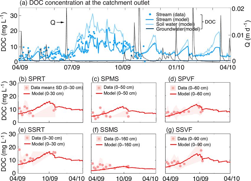
H. Wen et al.: The temperature and hydrology control on the production and export of DOC                                                  947

Figure 1. Attributes of the Susquehanna Shale Hills Critical Zone Observatory (SSHCZO): (a) surface elevation, (b) soil depth, and (c) soil
organic carbon (SOC). The surface elevation was generated from lidar topographic data (criticalzone.org/shale-hills/data), whereas soil
depths and SOC were interpolated using ordinary kriging based on field surveys with 77 and 56 sampling locations, respectively (Andrews
et al., 2011; Lin, 2006). The SOC distribution in panel (c) is further simplified using the high, uniform SOC (5 % v/v) in swales and valley
soils based on field survey information (Andrews et al., 2011). Swales and valley floor areas were defined based on surface elevation via field
survey and a 10 m resolution digital elevation model (Lin, 2006). Additional sampling instrumentation is shown in panel (b), including six
soil water sites (circles) and three soil T sites (squares).

portance of land cover in determining DOC terrestrial routing             though soil respiration is an important process, this study fo-
and lateral transport. Terrestrial and aquatic carbon processes           cuses on the net production and export of DOC.
have also been integrated into the Soil and Water Assessment
Tool (SWAT) to simulate aquatic DOC dynamics (Du et al.,
2019). These modules typically simulate individual reactions              2     Methods
without considering multicomponent reaction thermodynam-
                                                                          2.1    Study site: a small catchment with an intermittent
ics and kinetics.
                                                                                 stream
   In this context, the recently developed BioRT-Flux-PIHM
model (BFP, Biogeochemical Reactive Transport–Flux–Penn                   The Shale Hills catchment is a 0.08 km2 , V-shaped, first-
State Integrated Hydrologic Model) fills an important gap                 order watershed with an intermittent stream in central Penn-
by incorporating coupled elemental cycling, stoichiometry,                sylvania. It is forested with coniferous trees and is situated
and rigorous thermodynamics and kinetics (Bao et al., 2017;               on the Rose Hill shale formation. The annual mean air T
Zhi et al., 2019). We used the BFP to address the follow-                 is 9.8 ± 1.9 ◦ C (± SD) and the annual mean precipitation is
ing question: how do hydrology and T interact to deter-                   1029 ± 270 mm over the past decade. The watershed is char-
mine rates of DOC production and export at the catchment                  acterized by large areas of swales and valley floors with deep
scale? We applied the BFP to a temperate forest catchment                 and wet soils (Fig. 1b). These lowland soils contain more
in the Susquehanna Shale Hills Critical Zone Observatory                  SOC (∼ 5 % v/v) than the hillslopes and uplands (∼ 1 %
(SSHCZO). This small catchment (< 0.1 km2 ) has gentle to-                v/v; Fig. 1c).
pography with a network of shallow depressions or swales                     Soil water DOC samples were collected using lysimeters
that have high SOC and deep soils (detailed in Sect. 2). It               with a diameter of 5 cm installed at 10 or 20 cm intervals
is underlain by one type of lithology (shale) and land use                from the soil surface to a depth of hand-auger refusal, which
(forest), providing a useful test bed to evaluate biogeochem-             varied from 30 to 160 cm depending on soil thickness. There
ical and hydrological functions (Brantley et al., 2018). Pre-             were a total of six sampling locations (Fig. 1b), including
vious lab and field work have identified non-chemostatic C–               three at the south planar sites – valley floor (SPVF), mid-
Q patterns of DOC at SSHCZO that are attributable to dif-                 slope (SPMS), and ridgetop (SPRT) – and three at the swale
ferences in the hydrologic connectivity of organic-rich soils             sites – valley floor (SSVF), mid-slope (SSMS), and ridgetop
during different flow conditions (Andrews et al., 2011; Hern-             (SSRT). No soil water DOC samples were collected on the
don et al., 2015). SSHCZO has spatially extensive and high-               north side of the catchment. Stream water DOC samples were
frequency measurements of soil properties, hydrology, and                 collected daily in glass bottles at the stream outlet weir. All
biogeochemistry (Brantley et al., 2018). These data facilitate            soil water and stream water DOC samples were filtered to
detailed benchmarking of the BFP model and evaluation of                  0.45 µm using Nylon syringe filters and were analyzed with a
processes controlling DOC production and export. We ex-                   Shimadzu TOC-5000A analyzer (detailed in Andrews et al.,
pected that T and soil moisture would drive DOC produc-                   2011). Real-time soil T (every 10 min) was measured at the
tion in the soil, whereas DOC export and, thus, C–Q patterns              ridgetop, mid-slope, and valley floor (squares in Fig. 1b) us-
would be most related to hydrological connectivity. There-                ing automatic monitoring stations at depths of ∼ 0.10, 0.20,
fore, we predicted that DOC production and export might be                0.40, 0.70, 0.90, 1.00, and 1.30 m (Lin and Zhou, 2008).
asynchronous (i.e., not occurring at the same time) because
they respond differently to changes in T and hydrology. Al-

www.hydrol-earth-syst-sci.net/24/945/2020/                                                 Hydrol. Earth Syst. Sci., 24, 945–966, 2020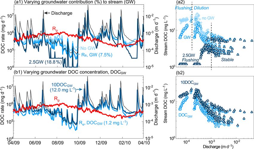
948                            H. Wen et al.: The temperature and hydrology control on the production and export of DOC

Figure 2. A schematic representation of major processes in the catchment reactive transport model BFP (BioRT-Flux-PIHM). Stream dis-
charge Q includes surface runoff QS , soil water interflow (lateral flow) QL , and groundwater flow QG . In the vertical direction, soil pores
are not saturated with water in the shallow unsaturated zone and water flows vertically until it reaches the saturated zone where water forms
interflows and moves laterally to the stream. Soil water total storage ST is the sum of water in the unsaturated (Su ) and saturated zones (Ss ).
Some water also recharges further into deeper groundwater. Within the soil zone, SOC decomposes and releases DOC, which also sorbs onto
the soil surface to become ≡ XDOC.

2.2   The BioRT-Flux-PIHM (BFP) model                                      tion in groundwater chemistry (Jin et al., 2014; Thomas et al.,
                                                                           2013; Kim et al., 2018). The QG is estimated using conduc-
                                                                           tivity mass-balance hydrograph separation (Lim et al., 2005).
BFP is the catchment reactive transport model of the general                  The BioRT module takes in water calculated at each
PIHM (Penn State Integrated Hydrologic Modeling System)                    time step to simulate reactive transport processes. BFM dis-
family of code (Duffy et al., 2014). The code includes three               cretizes the domain into prismatic elements and uses a finite
modules (Fig. 2): the surface hydrological module PIHM, the                volume approach based on mass conservation. The mass con-
land surface module Flux, and the multicomponent reactive                  servation governing equation for the reactive transport of a
transport module BioRT (Biogeochemical Reactive Trans-                     single solute m is as follows:
port). The code has been applied to simulate conservative
solute transport, chemical weathering, surface complexation,                     d(Sw,i θi Cm,i )
                                                                           Vi                     =
and biogeochemical reactions at the catchment scale (Bao                               dt
et al., 2017; Zhi et al., 2019; Li, 2019). Here, we only in-                      Ni,x
                                                                                  X               Cm,j − Cm,i
troduce the salient features that are relevant to this study;                            Aij Dij              − qij Cm,j + rm,i ,
readers are referred to earlier publications for further de-                    j =N
                                                                                                       lij
                                                                                    i,1
tails. Flux-PIHM separates the subsurface flow into active                   m = 1, np,                                                      (1)
interflow in shallow soil zones and groundwater flow deeper
than the soil-weathered rock interface. Note that this “deeper             where i and j represent the grid block i and the neighboring
groundwater” is the groundwater that actively interacts with               grid j ; the subscript x distinguishes between flow in the un-
the stream and shallow layer, not necessarily the water in the             saturated zone (infiltration and recharge) and saturated zone
deep groundwater aquifer. The PIHM module simulates hy-                    (recharge and lateral flow); V is the total bulk volume (m3 )
drological processes including precipitation, infiltration, sur-           of each grid block; Sw is the soil moisture (m3 water m−3
face runoff QS , soil water interflow (lateral flow) QL , and              pore volume); θ is porosity; C is the aqueous species con-
discharge Q (Fig. 2). The Flux module simulates processes                  centration (mol m−3 water); t is time (s); N is the index of
including solar radiation and evapotranspiration. Flux-PIHM                elements sharing surfaces; A is the grid interface area (m2 );
calculates water variables (e.g., water storage, soil moisture,            D is the diffusion/dispersion coefficient (m2 s−1 ); l is the dis-
and water table depth) in unsaturated and saturated zones                  tance (m) between the center of two neighboring grid blocks;
and assumes a no-flow boundary at the soil–bedrock inter-                  q is the flow rate (m3 s−1 ); rm is the kinetically controlled re-
face with high permeability contrast. In this version of Flux-             action rates (mol s−1 ) involving species m, which is the DOC
PIHM, the deeper groundwater flow QG is a separate input to                production rate from SOC decomposition at the grid block i;
the stream and is decoupled from the shallow soil water. This              and np is the total number of independent solutes.
is supported by field data that show negligible seasonal varia-

Hydrol. Earth Syst. Sci., 24, 945–966, 2020                                                 www.hydrol-earth-syst-sci.net/24/945/2020/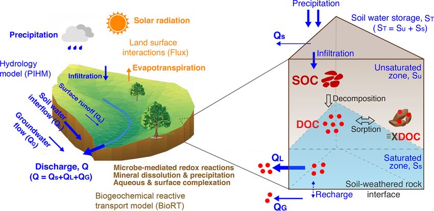
H. Wen et al.: The temperature and hydrology control on the production and export of DOC                                         949

2.3   DOC production and sorption                                   It depends on temperature but also on soil properties such as
                                                                    the clay content and the abundance of iron oxides (Kaiser et
In the model, DOC is produced by the decomposition of SOC           al., 2001; Conant et al., 2011). A Keq value of 100.2 was ob-
via the kinetically controlled reaction SOC(s) → DOC. With          tained by fitting the stream and soil water DOC data (detailed
abundant SOC and O2 in soils serving as electron donors and         in Sect. 2.4). The sum of [≡ X] and [≡ XDOC] represents
acceptors, a typical dual Monod kinetics can be simplified          the soil sorption capacity. A value ranging from 4.0 × 10⁻⁵
into zero-order kinetics with additional temperature and soil       to 6.0 × 10⁻⁵ mol g−1 soil was used for Shale Hills (Jin et
moisture dependence:                                                al., 2010; Li et al., 2017a) depending on the mineralogy in
                                                                    different zones of the catchment.
rp = kAf (T ) f (Sw ) ,                                      (2)
                                                                    2.4   Domain setup
where rp is the local DOC production rate in individual grids
(rm in Eq. 1, m is DOC); k is the kinetic rate constant of
                                                                    BFP is a model with full discretization in the horizontal
net DOC production (10−10 mol m−2 s−1 ) (Zhi et al., 2019;
                                                                    direction and partial discretization in the vertical direction
Wieder et al., 2014); and A is a lumped “surface area” (m2 ,
                                                                    with three layers: ground surface, unsaturated, and satu-
(2.5 × 10⁻³ m2 g−1 ) × (g of SOC mass)) that quantifies SOC
                                                                    rated zones. Although a new version of BFP explicitly in-
content and biomass abundance (Chiou et al., 1990; Kaiser
                                                                    cludes a groundwater zone, it was not released in time for
and Guggenberger, 2003; Zhi et al., 2019). The functions
                                                                    this work, so the groundwater fluxes were estimated sepa-
f (T ) and f (Sw ) describe the rate dependence on soil T
                                                                    rately. The study watershed was discretized into 535 pris-
and moisture, respectively. f (T ) follows a widely used Q10 -
                                |T −10|/10                          matic land elements and 20 stream segments using PIHMgis
based formation: f (T ) = Q10              , where Q10 quantifies   (http://www.pihm.psu.edu/pihmgis_home.html, last access:
the rate increases with T , with the superscript 10 referring to    11 February 2020), a GIS interface for BFP. The land el-
a T value of 10 ◦ C (Davidson and Janssens, 2006). Q10 in           ements are unstructured triangles with mesh sizes varying
the base case is set at 2.0, within the typical range of 1.2–3.8    from 10 to 100 m. The simulation domain was set up using
for forest ecosystems (Liu et al., 2017). The f (Sw ) has the       national datasets: the USGS National Elevation Dataset for
form f (Sw ) = (Sw )n in the base case, where n is the sat-         topography; the National Land cover Database for vegeta-
uration exponent with a value of 1.0, which is within the           tion distribution; the National Hydrography Dataset for wa-
typical range of 0.75–3.0 for most soils (Yan et al., 2018;         ter drainage network; the North American Land Data Assim-
Hamamoto et al., 2010). The dependence of production rates          ilation Systems Phase 2 (NLDAS-2) for hourly meteorologi-
on soil T and moisture have been described using multi-             cal forcing; and the Moderate Resolution Imaging Spectrora-
ple forms in existing studies (Davidson and Janssens, 2006;         diometer (MODIS) for leaf area index. In addition, extensive
Yan et al., 2018) and will be further explored via sensitiv-        characterization and measurement data at Shale Hills were
ity analysis, as detailed in Sect. 2.6. The SOC content typ-        used to define soil depth and soil mineralogical properties
ically decreases with depth (Billings et al., 2018; Bishop et       such as surface area and ion exchange capacity that are het-
al., 2004), although the specific pattern may vary with soil        erogeneously distributed across the catchment (Andrews et
texture, landscape position, vegetation, and climate (Jobbagy       al., 2011; Lin, 2006; Jin and Brantley, 2011; Jin et al., 2010;
and Jackson, 2000). The depth function of SOC at Shale Hills        Shi et al., 2013) (http://criticalzone.org/shale-hills/data/, last
has been observed to be exponential (Andrews et al., 2011),         access: 11 February 2020). Other soil matrix properties in-
which is typical of many soils (Billings et al., 2018; Currie       clude conductivity, porosity, and van Genuchten parameters.
et al., 1996). Totake this
                          into account, we use the equation        Soil macropores such as cracks, fractures, and roots can gen-
                       z
Cd (z) = C0 exp − bm , where Cd is SOC at depth z below             erate preferential flows. Their properties are represented us-
the surface; C0 is the SOC level at the ground surface, and         ing the area macropore fraction, depth, and conductivities.
bm quantified the decline rate with depth, which is set here to     They are parameterized based on values quantified in previ-
a value of 0.3 (Weiler and McDonnell, 2006).                        ous studies at Shale Hills (Shi et al., 2013; Lin, 2006), as
   DOC produced from SOC can also sorb on soils via the             shown in Fig. S1 and Table S1 in the Supplement.
following reaction: ≡ X+DOC ↔≡ XDOC, where ≡ X and                     Based on field measurements, the SOC content in swales
≡ XDOC represent the functional group without and with              and valley areas is relatively high (Andrews et al., 2011) and
sorbed DOC, respectively (Rasmussen et al., 2018). This re-         was set at 5 % (v/v solid phase) compared with 1 % in the
action is considered fast and is thermodynamically controlled       rest of the catchment (Fig. 1c). The clay minerals were set
with an equilibrium constant Keq that links the activity (here      at 23 % (v/v solid phase) along the ridgetop and 33 % at
approximated by concentrations) of the three chemicals via          the valley floor (Jin et al., 2010; Li et al., 2017a). The in-
         [≡XDOC]
Keq = [≡X][DOC]    . The DOC concentrations calculated from         put DOC concentrations in rainfall and groundwater (below
Eq. (1) were used to establish the concentrations of ≡ X and        soils) were set at reported medians of 0.6 and 1.2 mg L−1 ,
≡ XDOC. The Keq value represents the thermodynamic limit            respectively (Andrews et al., 2011; Iavorivska et al., 2016),
of the sorption, i.e., the sorption affinity of the soil for DOC.   as high-frequency DOC observations were not available. The

www.hydrol-earth-syst-sci.net/24/945/2020/                                          Hydrol. Earth Syst. Sci., 24, 945–966, 2020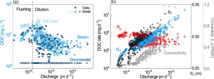
950                         H. Wen et al.: The temperature and hydrology control on the production and export of DOC

initial DOC concentration in soil water was set at 2.0 mg L−1 ,   ometry and the extent of connectivity, Ics /Width may vary
which was the average concentration from the six field sam-       from 0 to 1.0. A high Ics /Width value (i.e., high hydrologi-
pling locations in Fig. 1.                                        cal connectivity) indicates that a large catchment area is con-
                                                                  nected to the stream. To determine whether two grids are hy-
2.5     Model calibration                                         drologically connected, the spatial distribution of saturated
                                                                  water storage was Rused to calculate connectivity following
                                                                                       ∞
We used stream (daily) and soil pore water (biweekly) DOC         the equation Ics = 0 τ (h)dh and an algorithm in the litera-
concentration data from April to October 2009 for model cal-      ture (Allard, 1994; Western et al., 2001; Xiao et al., 2019).
ibration and the year 2008 as spin-up until a “steady state”      Here τ (h) is the probability of two grid blocks being con-
for both water and DOC was reached. The “steady state”            nected at a separation distance of h. Two grids are considered
here refers to a state where the inter-annual difference be-      “connected” if they are joined by a continuous flow path and
tween stored mass within the catchment is less than 5 % of        have saturated storages exceeding the threshold of the 75th
the total mass. The water input is precipitation, and its out-    percentile of saturated storage (over the whole catchment).
put is ET and discharge. The DOC mass input is from rain-         Note that Ics /Width here only quantifies the hydrological
fall, groundwater, and production, and the DOC output is the      connectivity in soils and does not reflect the groundwater in
export load at the stream outlet. The model performance was       shallow aquifers below the soil–bedrock interface.
evaluated using the monthly Nash–Sutcliffe efficiency (NSE)
(Nash and Sutcliffe, 1970) that quantified the residual vari-     2.6.2   DOC concentration–discharge relationships
ance of modeling output compared to measurements. The
general satisfactory range for monthly average outputs for        At the catchment scale, we differentiate the DOC produc-
hydrological models is NSE > 0.5 (Moriasi et al., 2007), and      tion rates and export rates. The production rate Rp is the
we used similar standards for biogeochemical solutes (Li et       sum of the local DOC production rate rp in individual grid
al., 2017a). To reproduce the DOC data, we first set the SOC      blocks (Eq. 2) across the whole catchment. The export rate
surface area A using a literature range of 10−3 –100 m2 g−1       Re is the product of discharge and the DOC concentration
(Zhi et al., 2019; Chiou et al., 1990; Kaiser and Guggen-         at the stream outlet. Total stored DOC is the difference be-
berger, 2003). We also set Keq using a literature range of        tween stream output and input from production, rainfall, and
100 –101 (Oren and Chefetz, 2012; Ling et al., 2006). Once        groundwater. The DOC input from the rainfall Rr (mg d−1 )
the simulated output captured the temporal trend of data, we      is the precipitation rate (m d−1 ) times the rainfall DOC con-
refined QG based on the estimation from hydrograph sep-           centration (6.0 × 10⁻⁴ mg m−3 = 0.6 mg L−1 × 10⁻³ L m−3 )
aration (Fig. S2) to capture the peaks of stream DOC con-         and the catchment drainage area (m2 ). The DOC input
centration, especially under low-discharge periods. Because       from groundwater Rg (mg d−1 ) is the total groundwater in-
not all soils are in contact with water, the calibrated sur-      flux (flow rate) times the groundwater DOC concentration
face area represents the effective solid–water contact area,      (1.2 mg L−1 ).
and is orders of magnitude lower than the reported SOC sur-          C–Q patterns were quantified using two complementary
face areas from laboratory experiments (Kaiser and Guggen-        approaches: the power law equation C = aQb (Godsey et
berger, 2003). The calibrated hydrological parameters are         al., 2009) and the ratio of the coefficients of variation of the
                                                                                                         CV[DOC]
mostly from Shi et al. (2013), except groundwater estima-         DOC concentration and discharge CV          Q
                                                                                                                  (Musolff et al.,
tion. Groundwater estimates were based on Li et al. (2017a)       2015). The slope of the power law equation b does not ac-
and further refined using conductivity mass-balance hydro-        count for the goodness of fit of the C–Q pattern itself. For
graph separation (Lim et al., 2005) and then by reproduc-         example, a slope of b = 0 would be considered chemostatic
ing the stream DOC concentration. In other words, stream          (i.e., relatively small variation of concentration compared
and groundwater chemistry data together helped constrain          with discharge), although high variability in solute concen-
the groundwater flow.                                             trations would in fact reflect a chemodynamic behavior (i.e.,
                                                                  solute concentrations are sensitive to changes in discharge).
2.6     Quantification of water and DOC dynamics                  We considered two general categories based on these met-
                                                                  rics (Musolff et al., 2015): if b values fell between −0.2 and
                                                                            CV[DOC]
2.6.1    Hydrological connectivity                                0.2 and CV     Q
                                                                                     1, C–Q patterns were considered chemo-
                                                                                                CV[DOC]
                                                                  static; values of |b| > 0.2 or CV Q
                                                                                                        ≥ 1, indicated a chemo-
Saturated soil water storage calculated from the model was        dynamic behavior. In the chemodynamic category, values of
used to quantify hydrological connectivity Ics /Width. With       b > 0.2 indicate flushing, whereas values of b < −0.2 indi-
“Width” defined as the average width of catchment in the          cate dilution. We used the MATLAB curve-fitting toolbox to
direction perpendicular to the stream (230 m), the term           obtain the best fit model parameters.
Ics /Width quantifies the average proportional width of the
catchment connected to the stream (e.g., Ics /Width = 0.10,
0.35, and 0.70 in Fig. S3). Depending on the catchment ge-

Hydrol. Earth Syst. Sci., 24, 945–966, 2020                                      www.hydrol-earth-syst-sci.net/24/945/2020/
H. Wen et al.: The temperature and hydrology control on the production and export of DOC 951
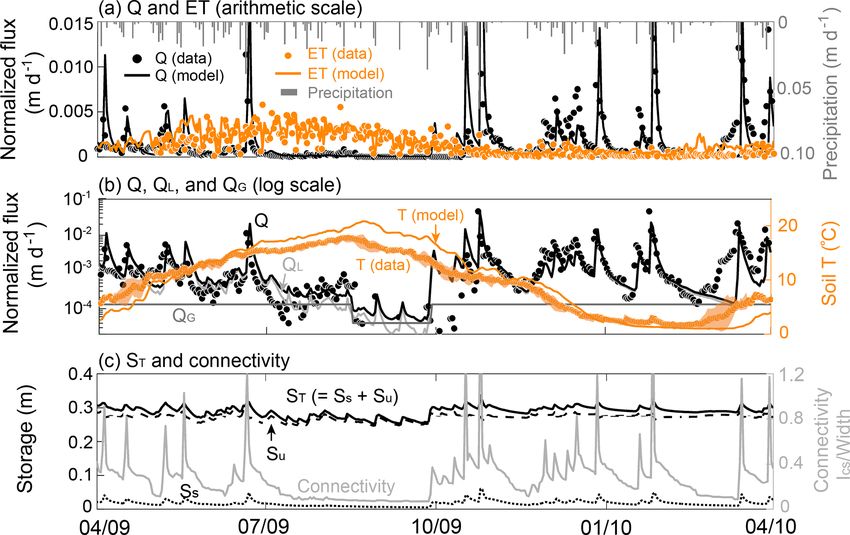
Figure 3. Temporal dynamics of (a) daily precipitation, stream discharge Q, and evapotranspiration ET on the arithmetic scale; (b) stream
discharge Q, soil water interflow QL , and groundwater QG on a logarithmic scale with soil T on an arithmetic axis (right); (c) soil water
storage ST (unsaturated water storage Su + saturated water storage Ss ) and hydrological connectivity Ics /Width. The yellow dots in panel (b)
represent the average soil T from three sampling locations (square symbols in Fig. 1b) with the shading reflecting variation in measurement.
Q was highly responsive to intense precipitation events in spring and winter. Note high soil T , high ET, low Ss , and lowIcs /Width during
July–August 2009. Stream discharge was primarily comprised of QL , except in July–October when the relative contribution of QG increased.
2.7 Sensitivity analysis trajectories rather than absolute values of f (Sw ) were com-
pared (Fig. S4b). The sensitivity of DOC sorption onto soils
We used a sensitivity analysis to explore the influence of soil was tested using Keq values of 0 (no sorption), 100.5 and
T and moisture in the DOC production kinetics. The Q10 101.0 .
|T −10|/10
in f (T ) = Q10 was explored using a minimum value The sensitivity of C–Q patterns and Re to changes in
of 1.0 (i.e., no dependence on T ) and a maximum value of groundwater was also tested with groundwater flow contri-
4.0 (Davidson and Janssens, 2006) (Fig. S4a), i.e., f (T ) = 1 bution and DOC concentration. The groundwater flow rates
and f (T ) = 4|T −10|/10 . The rate dependence on soil moisture were varied from negligible (QG = 0) to 2.5 times those of
was explored using the base case f1 (Sw ) = (Sw )n (increase the base case (QG = 3.3×10⁻⁴ and 1.0×10⁻⁴ m d−1 for the
behavior), and three additional functions (f2 , f3 , and f4 ) rep- wet and dry periods, respectively). The corresponding frac-
resenting the most commonly observed forms (Fig. S4b), in- tions (QG /Q) of groundwater flow to the total annual dis-
cluding decrease behavior, constant behavior, and threshold charge for the two cases were 0 % and 18.8 %, respectively.
behavior (Gomez et al., 2012; Yan et al., 2018): The groundwater DOC concentration (DOCGW ) was varied
the decrease behavior function was by 2 orders of magnitude (0.12 and 12.0 mg L−1 ). Results
from these analyses were compared with the base case, in
1 − Sw 0.77
f2 (Sw ) = , (3) which the groundwater contributed to 7.5 % of the total an-
0.6 nual streamflow at 1.2 mg L−1 .
the constant behavior function was
f3 (Sw ) = 0.65, (4) 3 Results
and the threshold behavior function was 3.1 Water dynamics
1.5
Sw
Sw ≤ 0.7 The total precipitation from 1 April 2009 to 31 March 2010
0.7
f4 (Sw ) = 1.5 (5) was 1130 mm. Stream discharge was highly responsive to in-
1−Sw
Sw > 0.7. tense precipitation events and was high (∼ 10−2 m d−1 ) in
1−0.7
spring and fall compared with summer with high soil T and
The constants in Eqs. (3)–(5) were selected to ensure sim- high ET (∼ 10−5 m d−1 ). The model captured the temporal
ilar averages of f (Sw ) across the whole Sw range such that dynamics of daily discharge, ET, and soil T with NSE values
www.hydrol-earth-syst-sci.net/24/945/2020/ Hydrol. Earth Syst. Sci., 24, 945–966, 2020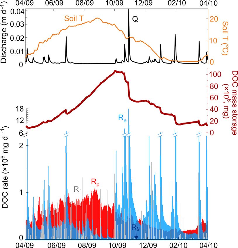
952                           H. Wen et al.: The temperature and hydrology control on the production and export of DOC

Figure 4. (a) Temporal dynamics of measured and simulated stream DOC concentrations as well as groundwater and soil water DOC. The
stream DOC (bright blue line) was from the soil water (light blue line) and groundwater QG (dark blue line). Under low-discharge conditions
(e.g., July–September), QG contributed a larger proportion of discharge and stream DOC was more similar to groundwater DOC. Under wet
conditions, stream DOC resembled soil water DOC from QL . (b–g) The local soil water DOC concentration for the six sampling locations
shown in Fig. 1b, including three planar (panels b–d) and three swale locations (panels e–g). The mean ±SD for each location was calculated
based on measurements at different depths with 10 or 20 cm intervals from the soil surface down to a depth of hand-auger refusal.

of 0.68, 0.72, and 0.62, respectively (Fig. 3a, b). The model           tions. High summer ET drove the catchment to drier con-
estimated that 47.5 % of annual precipitation contributed to            ditions, thereby decreasing the connectivity to the stream.
discharge, whereas the rest contributed to ET. The stream
discharge has three components: surface runoff QS , soil wa-            3.2   Temporal patterns of DOC concentrations
ter interflow QL (lateral flow), and groundwater flow QG
from the shallow subsurface that interacts with the stream              The model captured the general trend of stream DOC (NSE
(Fig. 2). On average, lateral flow QL is about 90.2 % and               of 0.55 for the monthly DOC concentration; Fig. 4). Under
surface runoff QS is about 2.3 %. Following the conductiv-              dry conditions (e.g., Q < 1.0×10⁻⁴ m d−1 ), QG contributed
ity mass-balance hydrograph separation (Lim et al., 2005),              substantially to Q (∼ 32 %–71 %; Fig. 3), and the stream
QG was estimated to be 1.3 × 10⁻⁴ and 4.0 × 10⁻⁵ m d−1                  DOC concentration reflected the mixing of groundwater and
for the wet and dry periods (August–September), which is                soil water (Fig. 4a), with a contribution from groundwater
equivalent to 6.9 % and 42.2 % of average stream discharge              DOC of 7 %–17 %. Under wet conditions, the stream DOC
at the corresponding times, respectively. Overall QG ac-                concentration overlapped with the soil water DOC concen-
counted for ∼ 7.5 % of the annual Q, similar to previously              tration (light blue line in Fig. 4). Only ∼ 1 %–8 % of stream
reported values (Li et al., 2017a; Hoagland et al., 2017). In           DOC was sourced from groundwater at these times.
the dry months from August to September, the stream was                    The temporal dynamics of soil water data showed rela-
almost dry with no visible flow, and the relative contribu-             tively small temporal variation compared with stream DOC
tion of groundwater to discharge was comparable to that of              (Fig. 4b, c, d, e, f, g), and local soil pools were not al-
QL (Fig. 3b). The unsaturated water storage Su was typically            ways hydrologically connected to the stream. The simulated
more than 10 times larger than the saturated storage Ss such            soil water DOC captured this small-variation trend with ac-
that the ST and Su curves almost overlapped (Fig. 3c). Ss was           ceptable overall model performance (i.e., NSE > 0.5), al-
negligible in the dry period (close to 0 m), contributing neg-          though the goodness of fit was lower in some locations, e.g.,
ligibly to the stream. Hydrological connectivity (Ics /Width)           a NSE value of 0.36 (SPRT), 0.42 (SPMS), 0.60 (SPVF),
covaried with Ss but showed significant temporal fluctua-               0.46 (SSRT), 0.40 (SSMS), and 0.51 (SSVF). The variation
                                                                        in model performance at different locations may arise from
                                                                        the lack of detailed information on local soil properties and

Hydrol. Earth Syst. Sci., 24, 945–966, 2020                                             www.hydrol-earth-syst-sci.net/24/945/2020/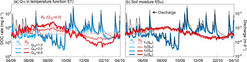
H. Wen et al.: The temperature and hydrology control on the production and export of DOC 953
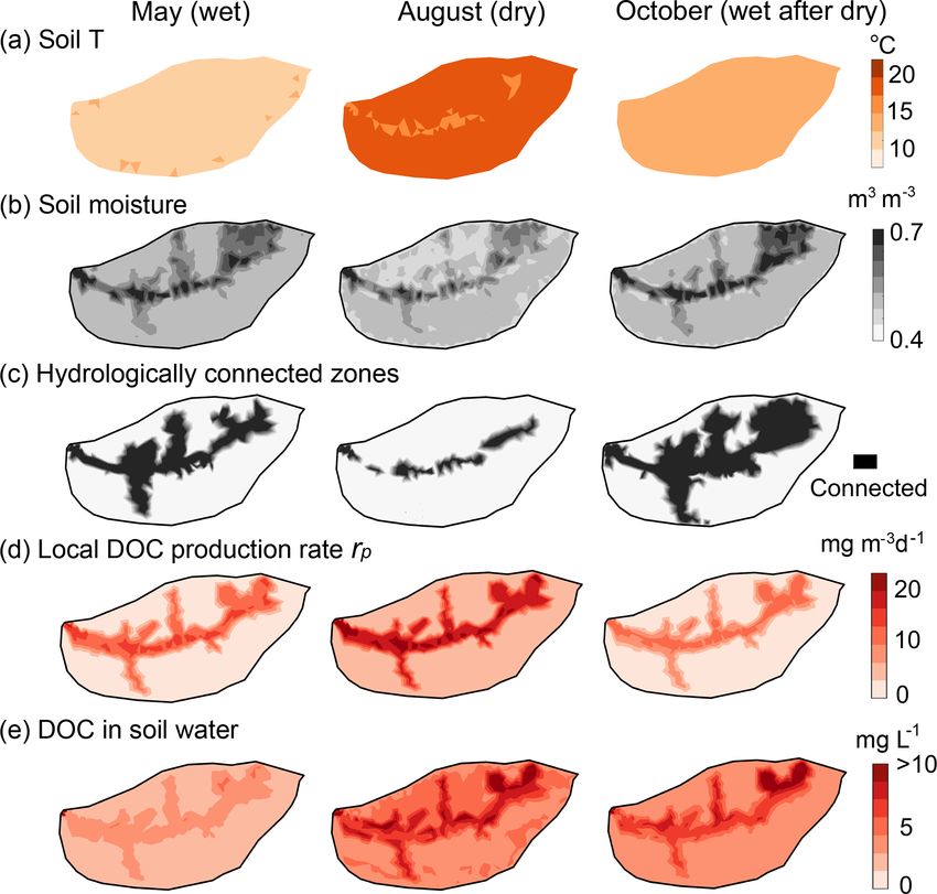
Figure 5. Spatial profiles in May (wet), August (dry), and October
(wet after dry) of 2009: (a) soil T , (b) soil moisture, (c) hydro-
logically connected zones, (d) local DOC production rates rp , and Figure 6. Temporal dynamics of DOC storage, influent rate (rainfall
(e) soil water DOC concentration. The soil DOC and rp were high Rr , groundwater Rg , production Rp ), and outflow rate (effluent Re )
in swales and the valley that had a relatively high soil water and at the catchment scale. The stored DOC mass (dark red line) was
SOC content (Fig. 1c). Although water content in August was rela- calculated as follows: (DOC influent rate − outflow rate) × time.
tively low compared with May and October, high soil T led to high The temporal Re dynamics mostly followed the trend of discharge
rp , with most DOC production and accumulation in zones that were (black line, top panel), whereas Rp mostly followed the trend of soil
disconnected from the stream. T (orange line, top panel).
organic carbon content. Although the model explicitly con-
sidered spatial heterogeneities such as topography and soil fold from May. The simulated soil water DOC concentration
properties, averaged values represented grid sizes from 10 increased by a factor of 2 across the whole catchment, espe-
to 100 m, and this local scale was large compared with the cially in hillslope and uplands on the north side, because the
field sampling size (e.g., lysimeters with a diameter of 5 cm). DOC produced was trapped in low soil moisture areas that
Geochemical processes are sensitive to local properties, in- were not hydrologically connected to the stream. This indi-
cluding SOC %, SOC surface area, and sorption sites, and cates that DOC samples collected on the south side may not
the representation of these properties was based on a few represent the DOC dynamics of the entire catchment, espe-
measurements that were only coarsely defined as ridgetop, cially in the summer and fall dry months. In October, rp de-
mid-slope, and valley floor. creased as soil cooled down, but increased precipitation and
decreased ET expanded the hydrologically connected zones
3.3 Spatial patterns and mass balance beyond swales and valley areas (Fig. 5c), promoting the des-
orption and the flushing of stored DOC. The soil water DOC
Spatial patterns vary between May (wet), August (dry), and concentration, however, remained high because of the large
October (wet after dry) (Fig. 5). In May, the average soil store of sorbed DOC produced during the antecedent dry
T was around 12 ◦ C with small spatial variations (< 3 ◦ C). times.
Most flow-convergent areas (valley areas and swales) were Figure 6 shows the catchment-scale DOC production and
well connected to the stream and had a high water content export rates and mass balance. Generally, the daily Rp (5.1 ×
(Fig. 5b, c). The distribution resembles that of SOC (Fig. 1c) 105 mg d−1 ) was greater than the daily Rr from rainfall (1.6×
and water content (Fig. 5b), with a high rp and soil water 105 mg d−1 ) or groundwater Rg (1.2 × 10⁴ mg d−1 ). During
DOC concentration in swales and valley. Low rp in rela- storm events, Rr occasionally exceeded Rp . Rp was generally
tively dry planar hillslopes and uplands led to a low soil water high in summer, despite low water storage. The export rate
DOC concentration. In August, the average soil T increased Re did not follow the temporal patterns of the total input rate
to around 20 ◦ C. The hydrologically connected zones shrank (Rp + Rr + Rg ) or Rp . Instead, it primarily followed the dis-
to the immediate vicinity of the stream, but rp increased 2- charge patterns: large rainfall events exported disproportion-
www.hydrol-earth-syst-sci.net/24/945/2020/ Hydrol. Earth Syst. Sci., 24, 945–966, 2020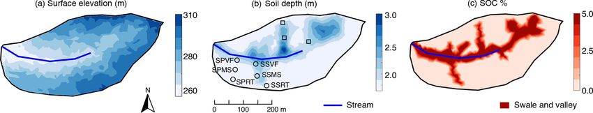
954                           H. Wen et al.: The temperature and hydrology control on the production and export of DOC

Figure 7. (a) Relationship of daily discharge (Q) with stream DOC concentration: open circles are simulations and filled circles with a black
outline are data. (b) Relationship of daily discharge (Q) with soil water storage ST , connectivity (Ics /Width), the catchment-scale DOC
export rate Re , and the DOC production rate Rp . At low Q, the stream water transitioned from organic-poor groundwater to organic-rich
water from the valley floor and swales, leading to a flushing (positive) pattern. At higher Q, the stream water shifted from organic-rich
soil water from swales and valley areas to lower DOC water from planar hillslopes and uplands, decreasing the stream DOC concentration
and resulting in a dilution C–Q pattern. Re increased by 2 orders of magnitude with increasing Q, whereas Rp varied within an order of
magnitude.

Figure 8. The catchment-scale DOC production rate Rp and export rate Re as a function of (a) soil T , (b) soil water storage ST , and
(c) hydrological connectivity (Ics /Width). Cross symbols are daily values in the base case. Rp increased with soil T and decreased slightly
with ST and connectivity. In contrast, Re increased with ST and connectivity but decreased with soil T . Re tended to decrease with soil T in
the hot, dry summer due to low discharge during that period.

ally high DOC, plummeting the DOC mass within the catch-                 The simulated C–Q relationships showed a general dilu-
ment. From the wet to dry period, as water levels dropped,                                                                   CV[DOC]
                                                                         tion behavior with the C–Q slope b = −0.23 and CV       Q
                                                                                                                                     =
DOC accumulated within the catchment (Fig. 5e, May to Au-                0.22, which was consistent with the general pattern exhib-
gust). During the dry-to-wet transition, as the catchment be-            ited in the field data (Fig. 7a). This C–Q pattern can be ex-
came wetter, the contributing areas expanded to the uplands              plained by the dynamics of different water sources with dif-
and the DOC was flushed out, reducing the overall DOC soil               ferent DOC contributing to the stream. At low discharges
pool to much lower values (Fig. 5e, August–October). The                 (< 1.8×10⁻⁴ m d−1 ) with small water storage (0.25–0.28 m)
DOC mass storage increased by 1.8 × 10⁶ mg over the year,                and connectivity (Ics /Width < 0.1) (Fig. 7b), the stream
which was about 1.0 % of the overall DOC production, indi-               DOC was a mix of organic-poor groundwater and organic-
cating a general mass balance at the catchment scale.                    rich swales and valley floor zones. As connectivity and dis-
                                                                         charge increased and the stream expanded, the contribution
3.4   C–Q patterns and rate dependence                                   of organic-rich swales increased, elevating the DOC con-
                                                                         centration to its maximum. Under even wetter conditions
The C–Q relationships showed a slightly positive correla-                with connectivity exceeding 0.1, the contribution from planar
tion at low Q followed by a negative correlation at higher               hillslopes and uplands with a lower DOC concentration in-
Q (Fig. 7a). The simulated C–Q relationship captured this                creased, diluting the organic-rich DOC from swales and val-
trend but overestimated the positive relationship at low Q.

Hydrol. Earth Syst. Sci., 24, 945–966, 2020                                              www.hydrol-earth-syst-sci.net/24/945/2020/
H. Wen et al.: The temperature and hydrology control on the production and export of DOC 955
Figure 9. Sensitivity analysis of temporal DOC rates for (a) soil temperature f (T ) and (b) soil moisture f (Sw ). A varying Q10 value in
f (T ) had a larger influence on Rp than varying f (Sw ). Neither f (T ) nor f (Sw ) had a significant influence on Re . Instead, Re mostly
followed the temporal trend of discharge, indicating the predominant control of hydrological conditions.
Figure 10. Sensitivity analysis of the sorption equilibrium constant Keq on (a) Rp and Re and on (b) DOC sorbed on soils averaged at
the catchment scale. High Keq led to more DOC sorbed on soils and, therefore, lower Re . However, Re showed similar temporal patterns
regardless of Keq .
ley areas. Daily Re correlated positively with ST , hydrolog- constant, SOC surface area, volume fraction, and biomass
ical connectivity, and Q, and increased by 2 orders of mag- amount could have similar effects (not shown here) because
nitude as Q rose by 3 order of magnitude. The variation of they are all multiplied in Eq. (2).
daily Rp with Q was small (105 –106 mg d−1 ) compared with Simulations showed that strong DOC sorption (Keq =
that of Re (Fig. 7b). Values of Rp depended more on soil 101.0 ) did not change Rp but lowered the stream DOC con-
T than on soil water storage and hydrological connectivity centration and resulted in smaller Re (Fig. 10a). DOC sorp-
(Ics /Width) (Fig. 8). In contrast, Re increased with soil wa- tion had little impact on Rp , but strong sorption decreased the
ter storage ST but notably decreased with soil T (> 17 ◦ C) magnitude of Re by 10 %–69 %. The sorbed DOC concen-
due to the low discharge during the hot and dry summer. tration differed by more than a factor of 3, with more sorbed
DOC with larger Keq values (Fig. 10b). Large amounts of
3.5 Sensitivity analysis sorbed DOC persisted until early fall, when large rainfall
events flushed out sorbed DOC and reduced DOC storage
3.5.1 Control of temperature, soil moisture, and (Fig. 6). This means that catchments can store large quan-
sorption tities of DOC, although the specific amount of DOC stored
depends on sorption capacity.
Higher Q10 values in f (T ) led to more pronounced season- Varying DOC production kinetics did not change the over-
ality in Rp (Fig. 9a). The Rp for Q10 = 4.0 was more than all C–Q patterns, although the magnitude of overall dilu-
4 times higher than that of Q10 = 1.0 in summer, and much tion changed slightly in cases with different f (T ) and Keq
lower in winter with low soil T (< 10 ◦ C). In contrast, the (Fig. 11). High Q10 values in f (T ) led to less dilution, due
temporal pattern of Re almost overlapped at different Q10 to more accumulated soil DOC in the dry period (low dis-
values, and it mostly followed the discharge dynamics (black charge) and, thus, more DOC flushing as discharge increased
line in Fig. 9). Daily Rp varied only slightly (within 15 %) in the dry-to-wet period. High Keq resulted in less dilution
with different f (Sw ) (Fig. S4b), while Re showed very lit- as the higher sorption capacity acts as a stronger buffer to
tle change (Fig. 9b). Although we varied Q10 from 1.0 to compensate for the concentration variations.
4.0 in f (T ), it is worth noting that varying the kinetic rate
www.hydrol-earth-syst-sci.net/24/945/2020/ Hydrol. Earth Syst. Sci., 24, 945–966, 2020956 H. Wen et al.: The temperature and hydrology control on the production and export of DOC
Figure 11. C–Q relationships under different (a) T , (b) f (Sw ), and (c) sorption equilibrium constants Keq for the two extreme cases. The
C–Q patterns were similar in all cases, although the extent of dilution slightly changed. This indicates potential factors other than reaction
kinetics and thermodynamics that regulate C–Q patterns.
Figure 12. Sensitivity analysis of groundwater on rates (Rp and Re ) and C–Q relationships: (a) scenarios with a different groundwater
volume contribution (%) to stream discharge and (b) scenarios with a different groundwater DOC concentration (DOCGW ). DOCGW and
GW (QG /Q) in the base case were 1.2 mg L−1 and 7.5 %, respectively. “2.5 GW” in panel (a) represents the case with 2.5 times QG
compared with the base case. Increases in the relative groundwater contribution lowered Re and shifted the C–Q pattern from an overall
dilution pattern to an overall flushing pattern; changing DOCGW had negligible influence on the DOC rates and C–Q patterns.
3.5.2 Groundwater control on DOC export tive groundwater contribution to streamflow for each case.
In contrast, varying the groundwater DOC concentration
As shown in Fig. 12, changing the groundwater volume con- (DOCGW ) by 2 orders of magnitude while keeping the same
tribution to stream (GW) had more significant impacts than groundwater contribution (GW) did not change C–Q pattern.
changing the groundwater DOC concentration (DOCGW ), Figure 13 summarizes the annual total Rp and Re in all
especially at low discharges (Q < 1.8 × 10⁻⁴ m d−1 ). In- sensitivity test scenarios. Annual Rp was more sensitive to
creasing the GW contribution from no GW to 2.5 GW (i.e., T than to Sw or sorption thermodynamics. Annual Re was
18.8 %) lowered stream DOC at low discharges, shifting the less sensitive to T variation, although it also increased with
C–Q pattern from overall dilution (or a chevron pattern) Q10 because a higher production led to higher DOC export.
to overall flushing (or flushing until stable). More specifi- Annual Rp also depended on f (Sw ), with the threshold func-
cally, the threshold that separated distinct phases of these tion f4 (Sw ) (Sect. 2.6) having the highest production rates.
segmented C–Q responses (Fig. 12a2) shifted from Q = However, Re did not follow the trend of Rp (Fig. 13b). Gen-
1.8 × 10⁻⁴ to about 1.0 × 10⁻³ m d−1 . This reflects the rela- erally, under the same hydrological conditions, a doubling
Hydrol. Earth Syst. Sci., 24, 945–966, 2020 www.hydrol-earth-syst-sci.net/24/945/2020/H. Wen et al.: The temperature and hydrology control on the production and export of DOC 957
Figure 13. Total annual Rp (red) and Re (blue) under two groundwater volume contribution conditions (QG /Q = 7.5 % and 18.8 %) for
three different variables: (a) soil T , (b) soil moisture, and (c) sorption equilibrium Keq . Rp was not influenced by a deeper groundwater
contribution, so there is only one curve for each variable. Rp has higher dependence on temperature than on soil moisture function form and
sorption capacity.
of Rp only led to about a 50 % increase in Re . Higher sorp- where water is limited and soil moisture can drop below 0.15
tion affinity (higher Keq ) did not change production rates but (Korres et al., 2015). This small variation is due to the ca-
could reduce DOC export by about 30 % due to high DOC pability of the shale-derived, clay-rich soils at Shale Hills to
storage in soils. High relative groundwater inputs (18.8 % hold water (Xiao et al., 2019). The influence of soil moisture
versus 7.5 %) lowered Re in all scenarios because more water on DOC production is likely higher in catchments with more
came from deeper organic-poor groundwater. pronounced seasonal changes and more fluctuations in soil
moisture.
This work also suggests that catchment-scale (Rp ) and
4 Discussion local-scale (rp ) production rates have different controls. The
rate law used at the local scale is measured at relatively small
This study revealed that DOC production was primarily regu- scales, i.e., 0.1–2.0 m in soil pedons (Bauer et al., 2008; Yan
lated by temperature, but the lateral export of DOC was con- et al., 2016). Our results show that even when the rate law
trolled by hydrological conditions. This work contributes to with an optimum soil moisture was used at the local scale
the growing body of research concluding that lateral carbon (f4 (Sw ) in Fig. S4b), the catchment-scale rates do not exhibit
flux is determined by water routing and hydrological con- maximum rates at an “optimal” soil moisture (Fig. 8), indi-
nectivity and only secondarily by biological activity (Zar- cating different controls at the local scale versus the catch-
netske et al., 2018). Although soil respiration and vertical ment scale. In addition, due to the spatial heterogeneities of
CO2 fluxes are closely related, this work focuses on the net T , soil moisture, and SOC content, the temporal variations
production and export of DOC because it has been studied of Rp and rp may be not consistent. The daily Rp spanned
and understood to a much lesser extent than soil respira- less than an order of magnitude with its maximum in the dry,
tion (Tank et al., 2018). To better appreciate the relative im- hot summer and its minimum in the wet, cold winter and
portance of land–water–atmosphere carbon fluxes, future re- spring (Fig. 6). Local-scale rp exhibited similar temporal dy-
search needs to fully integrate lateral DOC fluxes in concert namics but varied by more than 2 orders of magnitude, with
with vertical fluxes of CO2 across terrestrial and freshwater rapid production mostly in “hot spots” (swales and riparian
ecosystems. zones) with persistently high water and SOC content (Fig. 5).
Note that the local-scale rate laws are often used directly at
4.1 DOC production the catchment scale or at even larger scales (Crowther et al.,
2016; Conant et al., 2011; Fissore et al., 2009; Moyano et
The DOC production rate Rp depends more on T than on wa- al., 2012). This work suggests that although local-scale rate
ter storage or soil moisture. This finding is expected, as DOC laws have been developed extensively, direct extrapolation
production is biologically mediated and, thus, influenced by of rates from local to catchment scales can be misleading.
temperature and the metabolic dependence on temperature This speaks to the importance of understanding controls on
(Gillooly et al., 2001). Although the local-scale soil moisture biogeochemical transformation rates and developing reaction
varies from 0.40 at the ridgetop to 0.70 in swales and ripar- rate theories at the catchment scale for regional-scale and
ian zones (Fig. 5b), the averaged catchment-scale soil mois- global-scale simulations.
ture has relatively small variations across different seasons The simulations here suggest that DOC storage depends
in this temperate humid catchment (0.46 to 0.56 on average on the sorbing capacity of soils such that clay content and
over the whole catchment), especially compared with places
www.hydrol-earth-syst-sci.net/24/945/2020/ Hydrol. Earth Syst. Sci., 24, 945–966, 2020958 H. Wen et al.: The temperature and hydrology control on the production and export of DOC
the presence of organo-mineral aggregates might play a role catchment acts as a DOC producer in the summer and a DOC
in mediating DOC dynamics (Lehmann et al., 2007; Cincotta exporter in spring and winter when the soil is wetter.
et al., 2019). These findings indicate a strong climatic control over DOC
DOC production depends on catchment size, hydrogeo- production and export. In places where climate seasonality is
logic structure, vegetation, and climatic setting. Geomorpho- not as strong and catchments are hydrologically connected
logical and ecological processes have been shown to co- to streams throughout the year, we can expect to see DOC
generate systematic differences in the vertical and lateral export all year long and, therefore, much less asynchrony.
distribution of SOC and plant biomass, with a greater con- In places with strong seasonality, a few high-flow events
centration of organic carbon in the valley floor than in hill- can dominate the DOC export of the whole year. Under the
slopes in some catchments (Piney et al., 2018; Temnerud et Mediterranean climate with strong seasonality, for example,
al., 2016; Campeau et al., 2019; Thomas et al., 2016) and antecedent moisture conditions have been observed to be es-
enriched SOC in the uplands in other catchments (Herndon sential for understanding the temporal pattern of DOC and
et al., 2015). These differences may explain the large vari- nutrient (N ) export (Bernal et al., 2005, 2002). Hydrologi-
ation of stream DOC in catchments under diverse climate cal connectivity and water flow paths become dominant as
conditions (Moatar et al., 2017). The median stream DOC at subsurface saturation expands across valley floors and into
Shale Hills is relatively high (10.0 mg L−1 ), compared with hillslopes (Covino, 2017; Abbott et al., 2016).
3.0 mg L−1 in temperate humid catchments in Germany (Mu-
solff et al., 2018), 4.1 mg L−1 in some UK catchments with 4.3 Implications for vertical and lateral carbon fluxes
oceanic climate (Monteith et al., 2015), and 4.5 mg L−1 in
France (Moatar et al., 2017). It is also close to 9.5 mg L−1 This work focuses on DOC lateral fluxes and does not sim-
in boreal catchments in Sweden (Winterdahl et al., 2014), ulate the carbon loss through soil respiration and associated
and 8.1 mg L−1 measured in boreal wet and 10.5 mg L−1 in vertical CO2 fluxes, which has been the focus of some previ-
boreal dry catchments in Norway and Finland (de Wit et ous work (Brantley et al., 2018; Hasenmueller et al., 2015).
al., 2016). These differences suggest that climate, vegetation, Soil respiration is an important pathway of carbon flux that,
and landscape heterogeneity may together shape how much similar to DOC production, can be shaped by soil tempera-
DOC can be produced as well as when, where, and to what ture and moisture. Generally, warm temperature and medium
degree a hill is connected to a stream and the export of DOC soil moisture provide optimal conditions for microbial respi-
at different times. ration, leading to significant vertical losses of carbon during
summer months (Perdrial et al., 2018; Stielstra et al., 2015).
In contrast, low temperature and high soil moisture can hin-
4.2 Temporal asynchrony of DOC production and
der aerobic respiration and associated carbon losses as CO2
export
(Smith et al., 2018), effectively accumulating DOC until the
arrival of large storms. This pattern is consistent with ob-
The contrasting temporal patterns of simulated DOC produc- servations that the total CO2 release and DOC production
tion and export reflect the asynchronous nature of the two are positively correlated (Neff and Hooper, 2002). The de-
processes at the catchment scale. Local DOC production is pendence of DOC production and export on soil T and soil
influenced by the seasonal pattern of soil T , whereas the moisture might also hold true for soil respiration. Conversely,
export is predominantly controlled by precipitation events as part of the sorbed DOC may be respired by microbes into
and antecedent conditions that modulate the degree to which CO2 , our model might overestimate the DOC accumulation
DOC production zones are hydrologically connected to the in the catchment, especially in summer.
stream. This differs from studies showing the synchroniza- This work does not consider the transport of particulate or-
tion of DOC production and export in temperate climatic re- ganic carbon (POC) in soil water and stream water, although
gions at soil pedons (Michalzik et al., 2001). This may be due POC can play an important role in the carbon budget and bio-
to the relatively short water residence time and high connec- geochemical cycles in some cases (Ludwig et al., 1996; Diem
tivity at the pedon scale. The temporal asynchrony between et al., 2013). In Shale Hills, DOC comprises a major fraction
DOC production and export is therefore strongly influenced (between 70 % and 80 %) of the total organic carbon export
by the seasonality of temperature and precipitation, which is (Jordan et al., 1997). Similar patterns have been reported for
shaped by local climate. At Shale Hills the wet winter and organic carbon export at the global scale (Alvarez-Cobelas
spring happens to be the cold season, whereas the dry sum- et al., 2012). However, POC export can be significant in an-
mer is hot. In the summer, the catchment essentially produces thropogenically impacted areas (Correll et al., 2001; Matts-
and stores DOC in soil water and soil surfaces and waits for son et al., 2005) with significant disturbance (Abbott et al.,
the arrival of the next storm to export. In other words, low 2016). They follow a different temporal pattern from DOC,
hydrological connectivity in the summer imposes a lag pe- due to different sources, transport mechanisms, and sensi-
riod with respect to DOC export such that the DOC we see tivity to hydrologic variations (Dhillon and Inamdar, 2014;
today is often the DOC produced a while ago. As such, the Alvarez-Cobelas et al., 2012).
Hydrol. Earth Syst. Sci., 24, 945–966, 2020 www.hydrol-earth-syst-sci.net/24/945/2020/You can also read