Terrestrial or marine - indications towards the origin of ice-nucleating particles during melt season in the European Arctic up to 83.7 N - Recent
←
→
Page content transcription
If your browser does not render page correctly, please read the page content below
Atmos. Chem. Phys., 21, 11613–11636, 2021
https://doi.org/10.5194/acp-21-11613-2021
© Author(s) 2021. This work is distributed under
the Creative Commons Attribution 4.0 License.

Terrestrial or marine – indications towards the origin of
ice-nucleating particles during melt season in the
European Arctic up to 83.7◦ N
Markus Hartmann1 , Xianda Gong1,c , Simonas Kecorius1 , Manuela van Pinxteren2 , Teresa Vogl1,a , André Welti1,b ,
Heike Wex1 , Sebastian Zeppenfeld2 , Hartmut Herrmann2 , Alfred Wiedensohler1 , and Frank Stratmann1
1 Experimental  Aerosol and Cloud Microphysics, Leibniz Institute for Tropospheric Research, 04318, Leipzig, Germany
2 Atmospheric  Chemistry, Leibniz Institute for Tropospheric Research, 04318, Leipzig, Germany
a now at: Remote Sensing and The Arctic Climate System, Leipzig Institute for Meteorology,

University of Leipzig, 04103, Leipzig, Germany
b now at: Finnish Meteorological Institute, Helsinki, Finland
c now at: Center for Aerosol Science and Engineering, Department of Energy, Environmental and Chemical Engineering,

Washington University in St. Louis, St. Louis, USA

Correspondence: Markus Hartmann (markus.hartmann@tropos.de)

Received: 24 November 2020 – Discussion started: 26 November 2020
Revised: 27 May 2021 – Accepted: 27 May 2021 – Published: 4 August 2021

Abstract. Ice-nucleating particles (INPs) initiate the primary     enrichment factor (EF) varied mostly between 1 and 10, but
ice formation in clouds at temperatures above ca. −38 ◦ C          EFs as high as 94.97 were also observed. Filtration of the
and have an impact on precipitation formation, cloud opti-         seawater samples with 0.2 µm syringe filters led to a signif-
cal properties, and cloud persistence. Despite their roles in      icant reduction in ice activity, indicating the INPs are larger
both weather and climate, INPs are not well characterized,         and/or are associated with particles larger than 0.2 µm. A clo-
especially in remote regions such as the Arctic. We present        sure study showed that aerosolization of SML and/or seawa-
results from a ship-based campaign to the European Arc-            ter alone cannot explain the observed airborne NINP unless
tic during May to July 2017. We deployed a filter sampler          significant enrichment of INP by a factor of 105 takes place
and a continuous-flow diffusion chamber for offline and on-        during the transfer from the ocean surface to the atmosphere.
line INP analyses, respectively. We also investigated the ice      In the fog water samples with −3.47 ◦ C, we observed the
nucleation properties of samples from different environmen-        highest freezing onset of any sample. A closure study con-
tal compartments, i.e., the sea surface microlayer (SML), the      necting NINP in fog water and the ambient NINP derived from
bulk seawater (BSW), and fog water. Concentrations of INPs         the filter samples shows good agreement of the concentra-
(NINP ) in the air vary between 2 to 3 orders of magnitudes at     tions in both compartments, which indicates that INPs in the
any particular temperature and are, except for the tempera-        air are likely all activated into fog droplets during fog events.
tures above −10 ◦ C and below −32 ◦ C, lower than in midlat-       In a case study, we considered a situation during which the
itudes. In these temperature ranges, INP concentrations are        ship was located in the marginal sea ice zone and NINP lev-
the same or even higher than in the midlatitudes. By heat-         els in air and the SML were highest in the temperature range
ing of the filter samples to 95 ◦ C for 1 h, we found a sig-       above −10 ◦ C. Chlorophyll a measurements by satellite re-
nificant reduction in ice nucleation activity, i.e., indications   mote sensing point towards the waters in the investigated re-
that the INPs active at warmer temperatures are biogenic.          gion being biologically active. Similar slopes in the temper-
At colder temperatures the INP population was likely dom-          ature spectra suggested a connection between the INP popu-
inated by mineral dust. The SML was found to be enriched           lations in the SML and the air. Air mass history had no influ-
in INPs compared to the BSW in almost all samples. The             ence on the observed airborne INP population. Therefore, we

Published by Copernicus Publications on behalf of the European Geosciences Union.
11614                                                                              M. Hartmann et al.: Terrestrial or Marine

conclude that during the case study collected airborne INPs        son to clouds at similar altitudes in other parts of the globe
originated from a local biogenic probably marine source.           (Costa et al., 2017), which might be due to a lack of ice-
                                                                   nucleating particles (INPs). INPs are the catalyst needed for
                                                                   the primary ice formation at temperatures relevant for mixed-
                                                                   phase clouds and are thus essential to induce the freezing of
1   Introduction                                                   supercooled liquid cloud droplets.
                                                                      As INPs can directly affect the phase state of the cloud,
The Arctic is more sensitive to climate change than any other      their abundance and efficiency to initiate freezing also affects
region on Earth, and changes are proceeding at an unprece-         precipitation, lifetime, and the radiative effects of clouds
dented pace and intensity (Serreze and Barry, 2011). The in-       (e.g., Loewe et al., 2017; Prenni et al., 2007; Ovchinnikov
crease of the Arctic surface air temperature, the most promi-      et al., 2014; Solomon et al., 2015). Solomon et al. (2018)
nent variable to indicate Arctic change, exceeds the warm-         even state that the influences of INPs regarding the radiative
ing in midlatitudes by about 2 K (Wendisch et al., 2017;           properties of Arctic clouds are more important than those of
Overland et al., 2011; Serreze and Barry, 2011). This en-          cloud condensation nuclei (CCN). This underlines the im-
hanced warming phenomenon is referred to as Arctic amplifi-        portance of gaining quantitative knowledge about the abun-
cation (AA). Arctic peculiarities together with multiple feed-     dance, properties, nature, and sources of Arctic INPs.
back mechanisms are known to contribute to the enhanced               Several previous studies have reported that marine as well
sensitivity of the Arctic (Wendisch et al., 2017). And, while      as terrestrial sources contribute to Arctic INPs ice active at
the individual processes are known, the relative contribution      temperatures above approximately −15 ◦ C. For the marine
of each process, their strengths, and the interlinkage lead-       environment, it was found that especially the sea surface
ing to AA are still a field of ongoing research (Serreze and       microlayer (SML) can be highly ice active (Alpert et al.,
Barry, 2011; Pithan and Mauritsen, 2014; Cohen et al., 2020;       2011a, b; Bigg, 1996; Bigg and Leck, 2008; Irish et al.,
Wendisch et al., 2017).                                            2017, 2019b; Knopf et al., 2011; Leck and Bigg, 2005;
   Aerosol particles are a key factor in cloud formation and       Schnell and Vali, 1976; Wilson et al., 2015; Zeppenfeld et al.,
can alter the microphysical properties of clouds (Pruppacher       2019). Especially marine microorganisms such as bacteria
and Klett, 2010). The formation of clouds is further promoted      and algae as well as their exudates are thought to be the
by the increase in near-surface water vapor concentration due      source for the INPs. Connections to biological processes like
to the extended open water areas. Clouds and their properties      plankton blooms have been made (Creamean et al., 2019).
are essential for the energy budget of the Arctic boundary         Another recent publication by Kirpes et al. (2019) found
layer. Arctic clouds are often at low levels, and they tend to     that locally produced open leads are the dominant aerosol
warm the surface below the clouds (Intrieri, 2002; Shupe and       source in winter. The emitted sea spray aerosol particles
Intrieri, 2004) and consequently cause more sea ice to melt        were found to possess organic coatings, consisting of marine
(Vavrus et al., 2011). An increased cloud cover as well as the     saccharides, amino acids, fatty acids, and divalent cations.
accompanying downward longwave radiation also prevents             These substances are known from exopolymeric secretions
new sea ice from growing again, reducing the sea ice cover in      produced by sea ice algae and bacteria, which, as mentioned
the following seasons (Liu and Key, 2014; Park et al., 2015).      before, are thought to be responsible for the ice activity in
   The visible manifestation of the Arctic climate change is       seawater. Studies on INPs at coastal sites tend to find influ-
the perennial sea ice cover decline, which has intensified         ences from marine and terrestrial sources, often with a con-
over the last decade (Lang et al., 2017; Kwok et al., 2009).       tribution of biological INPs and seasonal changes (Creamean
The decline in sea ice results in an overall increase in ma-       et al., 2018; Šantl-Temkiv et al., 2019; Wex et al., 2019). For
rine biological activity, which may give rise to new sources       terrestrial sources, mineral dust itself is known to be relevant
for aerosol particles and/or alter existing ones (Arrigo et al.,   for lower temperatures (Sanchez-Marroquin et al., 2020), but
2008). Equivalently to the marine environment, the thaw-           Tobo et al. (2019) showed for glacial outwash material that
ing of permafrost increases the terrestrial biological activity    dust can be the carrier for biological material, which is more
(Hinzman et al., 2005) and presumably the emission of pri-         ice active than the dust alone. Highly ice-active biological
mary aerosol particles and/or particle precursors (Creamean        INPs have also been found in Arctic ice cores from up to
et al., 2020).                                                     500 years ago (Hartmann et al., 2019). Also millennia-old
   A number of studies showed that mixed-phase clouds pre-         permafrost soil was found to contain biological INPs that
vail, existing in the temperature range between 0 and −38 ◦ C,     can be mobilized into the atmosphere, lakes, rivers, and the
in the Arctic (e.g., Intrieri, 2002; Pinto, 1998; Shupe et al.,    ocean when the Permafrost thaws (Creamean et al., 2020).
2006, 2011; Turner, 2005). These clouds, which are com-            This highlights the importance of biological INPs, especially
posed of a mixture of supercooled droplets and ice crys-           in the changing Arctic environment.
tals, typically extend over large areas and display extraordi-        Despite past significant efforts and increase in knowledge,
nary longevity despite their microphysically unstable nature.      we still lack quantitative insights concerning the abundance,
These clouds show a lower degree of glaciation in compari-         the properties, and sources of Arctic INPs. Especially con-

Atmos. Chem. Phys., 21, 11613–11636, 2021                                          https://doi.org/10.5194/acp-21-11613-2021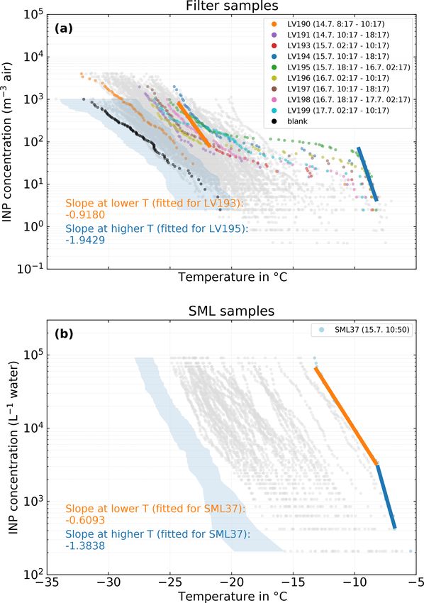
M. Hartmann et al.: Terrestrial or Marine 11615
cerning the last point, the relative importance of marine vs.
terrestrial sources is still debated. Therefore, open questions
addressed in this paper are outlined:
– What is the abundance of Arctic INPs and in what tem-
perature range can they nucleate ice?
– What is the nature of Arctic INPs (biogenic material vs.
mineral dust)?
– What is the origin of Arctic INPs (local vs. long range
transport, marine vs. terrestrial)?
Our findings are constrained to the season and region in
which measurements took place. They will nevertheless con-
tribute to a better understanding concerning Arctic INPs and
their potential effects on Arctic clouds. Furthermore, we pro-
vide valuable data for evaluating and driving atmospheric
models in a region which is still heavily undersampled.
2 Methods
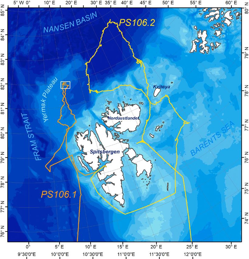
2.1 Campaign overview Figure 1. Overview of the main expedition area of the Polarstern
cruises PS106.1 and PS106.2. Figure taken from Macke and Flores
The expedition PS106 of the research vessel Polarstern (2018).
(Knust, 2017) was conducted between the end of May and
mid-July 2017 in the Arctic Ocean (Wendisch et al., 2019).
94.82 % ± 6.09 %, and p = 1006.84 hPa ± 5.12 hPa. Dur-
The measurements were performed as part of the PASCAL
ing the time within the ice pack, the averages of these
(Physical Feedbacks of Arctic Boundary Layer, Sea Ice,
parameters were as follows: Tair = −1, 37 ◦ C ± 1.50 ◦ C,
Cloud and Aerosol) campaign in the framework of the Ger-
RH = 94.35 % ± 4.54 %, and p = 1011.27 hPa ± 8.52 hPa;
man Arctic Amplification: Climate Relevant Atmospheric
out of the ice pack, Tair = 4.75 ◦ C ± 3.65 ◦ C, RH =
and Surface Processes, and Feedback Mechanisms (AC)3
88.03 % ± 11.27 %, and p = 1012.92 hPa ± 4.89 hPa.
project.
For further details on the measurement strategy as well
The first leg (PS106.1) started on 24 May in Bremerhaven
as the meteorological, sea ice, and cloud conditions during
(Germany) and ended on 21 June in Longyearbyen (Sval-
PASCAL, we refer the reader to Wendisch et al. (2019) and
bard) and featured a 10 d ice floe camp that was set up be-
the PS106 cruise report by Macke and Flores (2018).
tween 5 and 14 June 2017. The main area of investigation
was the Arctic Ocean a few hundred kilometers northwest of
2.2 Sample collection
Svalbard (see Fig. 1).
The expedition continued with its second leg (PS106.2) In order to gain a comprehensive insight into the abundance
on 23 June from Lonyearbyen and ended on 20 July in and nature of INPs in the Arctic during summertime, sam-
Tromsø (Norway). In comparison to PS106.1, the second leg ples from different compartments were taken. These included
focused on the area northeast of Svalbard, went up to higher atmospheric, bulk seawater (BSW), sea surface microlayer
latitudes (up to 83.7◦ N), and the vessel did not stop for ex- (SML), and fog samples. All samples were stored on the ves-
tended stays at an ice floe. sel directly after sampling in a cold room at −20 ◦ C, and
As an overview about the meteorological situation dur- it was ensured that the samples stayed below 0 ◦ C during
ing the campaign, Fig. S1 in the Supplement shows transport to the Leibniz Institute for Tropospheric Research
the frequency distributions for all meteorological parame- (TROPOS), where they were stored at −24 ◦ C until they
ters that were continuously measured on Polarstern. The were analyzed.
mean and standard deviation of air temperature (Tair ), rel-
ative humidity (RH), and atmospheric pressure (p) are 2.2.1 Filter sampling
given in the following: for the whole first leg they
are Tair = −0.01 ◦ C ± 4.21 ◦ C, RH = 90.70 % ± 10.62 %, Aerosol particles were sampled using a low-volume filter
and p = 1016.36 hPa ± 7.48 hPa, whereas for the second sampler (LVS; DPA14 SEQ LVS, DIGITEL Elektronik AG,
leg the parameters were Tair = 0.22 ◦ C ± 2.71 ◦ C, RH = Volketswil, Switzerland) with a PM10 inlet (DPM10/2.3/01,
https://doi.org/10.5194/acp-21-11613-2021 Atmos. Chem. Phys., 21, 11613–11636, 2021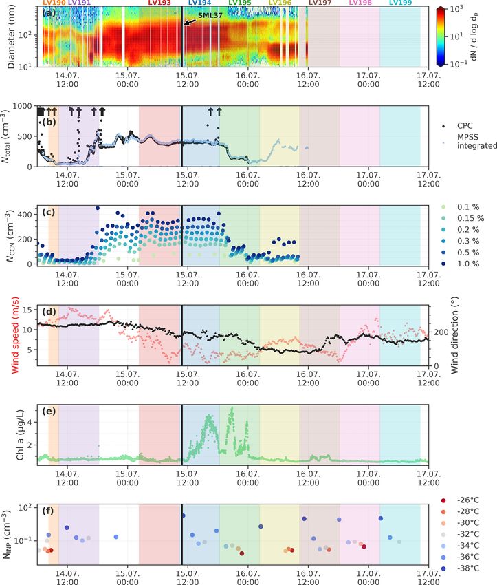
11616                                                                             M. Hartmann et al.: Terrestrial or Marine

DIGITEL Elektronik AG, Volketswil, Switzerland). The              2.2.3    Fog sampling
sampler was located on top of a measurement container
placed on the starboard side of the monkey island (ca. 30 m       Fog was collected with the Caltech Active Strand Cloud Col-
above sea level). It was operated with an average volumet-        lector Version 2 (CASCC2; described in Demoz et al., 1996).
ric flow of 27.9 L min−1 . It should be noted that our flow       The CASCC2 is a non-selective sampler that catches hy-
rate is lower than the standardized flow rate for PM10 in-        drometeors by impaction on Teflon® strands (508 µm diame-
lets; hence, our cutoff diameter is higher than 10 µm (ca.        ter). Droplets caught on the strands are gravitationally chan-
11.7 µm). The LVS was routinely operated with an 8 h sam-         neled into a Nalgene bottle. The instrument operates with a
pling period, which results in a total sampled air volume of      flow rate of approximately 5.3 m3 min−1 , resulting in a 50 %
13.4 m3 per filter sample. On 4 measurement days, the 8 h         lower cutoff size of approximately 3.5 µm. During daytime
cycle was replaced by a 2 h cycle to study possible diurnal       on leg 1 the sampler turned on every time the visibility de-
variation. The filter sampler features sealed storage cassettes   creased significantly and was running continuously during
and an automated filter change that allows for unsupervised       the night. On leg 2 the sampler was running continuously,
sampling for multiple days. The samples were collected on         and the sample bottle was changed whenever a significant
polycarbonate pore filters (Nuclepore® , Whatman™; 0.2 µm         amount of sample material was collected and after the fog
pore size, 47 mm diameter). Usually 12 filters were prepared      event was over. In all cases the sampler was rinsed with ultra-
and put in place inside the sampler. Two field blanks were        pure water after a fog event was sampled and after the sample
taken on each leg and were used to define the lower limit of      bottle was changed. During the entire campaign, 22 samples
observable NINP . A list of the almost 200 filter samples can     were collected, with about two-thirds of them on the second
be found in Table S1 in the Supplement. The filter-derived        leg alone. A list of all fog samples can be found in Table S3
NINP levels are also part of the overview of global shipborne     in the Supplement.
INP measurements by Welti et al. (2020).
                                                                  2.3     INP analysis
2.2.2   Bulk seawater and sea surface microlayer
        sampling                                                  2.3.1    Sample preparation
Seawater samples were taken from different environments,          Samples stored at −24 ◦ C were thawed only to perform the
i.e., ice-free ocean, marginal ice zone (MIZ), open leads         measurements. The measurements were performed on the
within the ice pack, or from melt ponds. In the case of the       same day as the thawing, and the remaining sample material
first three points, the samples were taken a few hundred me-      was refrozen at the end of the day on which the measure-
ters away from the position of Polarstern using a Zodiac          ments were completed.
boat, while the melt ponds on the ice floe could be reached          The polycarbonate filters were put in a centrifuge tube
on foot. BSW samples were typically taken from a depth of         along with 3 mL of ultrapure water (type 1; Direct-Q® 3
1 m with the help of a sealable bottle on a telescopic rod,       water purification system, Merck Millipore, Darmstadt, Ger-
with the exception of shallow melt ponds, where the samples       many) and were shaken in an oscillating shaker for 15 min
were taken near the ground (for details, see Zeppenfeld et al.,   in order to extract the particles from the filter and bring
2019). SML samples were collected with a glass plate sam-         them into suspension. Then 100 µL of that suspension was re-
pler (Zeppenfeld et al., 2019; Van Pinxteren et al., 2017). The   moved for the analysis with the Leipzig ice nucleation array
glass plate is dipped into the water body, slowly withdrawn,      (LINA; described in Sect. 2.3.3). For the analysis with the ice
and the surface film, which clings to the sides of the glass      nucleation droplet array (INDA; described in the Sect. 2.3.4),
plate, is wiped off the plate into a sample container with a      the remaining 2.9 µL of the suspension was made up to a to-
Teflon® wiper.                                                    tal of 6 mL with ultrapure water and shaken again as before.
   The seawater sampling was conducted on a daily basis.          The reason for this procedure is to use as little water as vi-
The SML and bulk seawater samples were taken at the same          able, i.e., to dilute the sample as little as possible.
time and location with the only exceptions being shallow             Sea and fog water samples did not require any preparation
melt ponds where no samples from 1 m depth could be taken         and could be directly measured with either setup.
as well as days with harsh weather when no surface film
could form; 42 SML samples and 42 bulk seawater samples           2.3.2    Test for heat-labile INPs
were collected during the campaign. A further description
of the seawater sampling and a chemical and microbiologi-         After the initial measurement, arbitrarily selected samples
cal analysis of the samples can be found in Zeppenfeld et al.     were chosen to test for the presence of heat-labile INPs in
(2019). A list of the seawater samples can be found in Ta-        the samples. The sample solution was sealed in a centrifuge
ble S2 in the Supplement.                                         tube and placed in an oven. The sample was heated at 95 ◦ C
                                                                  for 1 h and subsequently analyzed with the LINA device (de-
                                                                  scribed in Sect. 2.3.3).

Atmos. Chem. Phys., 21, 11613–11636, 2021                                          https://doi.org/10.5194/acp-21-11613-2021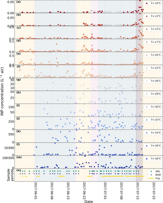
M. Hartmann et al.: Terrestrial or Marine                                                                                  11617

2.3.3   Leipzig ice nucleation array (LINA)                        top-mounted camera took pictures at 0.1 ◦ C intervals. The
                                                                   images were then again evaluated with a custom Python al-
LINA is a droplet-freezing assay (DFA), the design of which        gorithm for Nf in order to derive fice (T ). INDA was used
is based on a DFA called BINARY by Budke and Koop                  for measurements of SML and BSW samples as well as for
(2015). An array of 90 droplets with a typical volume of 1 µL      fog water.
of the sample suspension is placed onto a hydrophobic glass
slide (40 mm diameter). Each droplet is within its individual      2.3.5    INP number concentrations NINP
compartment made from a perforated, anodized aluminum
plate and covered with another glass slide. In this way it         Cumulative number concentrations of INPs per volume of
can be ensured that droplets do not interact during the freez-     sample as a function of temperature were calculated for each
ing process, e.g., via ice seeding by frost splintering or the     experiment utilizing the equation given in Vali (1971):
Bergeron–Wegener–Findeisen process. Furthermore, droplet                         − ln(1 − fice )
                                                                   NINP (T ) =                                                (1)
evaporation is minimized. At a cooling rate of 1 ◦ C min−1 ,                         Vdrop
the sample droplets are cooled by a 40 × 40 mm2 Peltier el-
ement inside a freezing stage (LTS120, Linkam Scientific           with fice = Nfrozen (T )
                                                                                  Ntotal , where Ntotal is the number of droplets,
Instruments, Waterfield, UK). The freezing stage is coupled        and Nfrozen (T ) is the number of frozen droplets at tempera-
with a cryogenic water circulator (F25-HL, Julabo, Seelbach,       ture T . With the given number of droplets (Ntotal = 90) and
Germany) in order to achieve temperatures below −25 ◦ C            volume (Vdrop = 1 µL), the upper and lower limits of the de-
down to the temperature at which homogeneous freezing              tectable range of LINA are 1.12 × 10⁴ and 4.5 × 10⁶ L−1
occurs naturally, i.e., −38 ◦ C. A thin layer of squalene oil      (water), respectively, whereas 2.1 × 10² and 9.1 × 10⁴ L−1
thermally connects the Peltier element and the glass slide         (water), respectively, are the limits for INDA (Ntotal = 96;
with the droplets on top. The freezing stage itself consists       Vdrop = 50 µL). The temperature values of the seawater sam-
of a gas-tight aluminum housing, which is purged with dry          ples were corrected for freezing-point depression due to the
particle-free air during the measurement. LED dome lighting        salt content as described in Koop and Zobrist (2009).
(SDL-10-WT, MBJ-Imaging GmbH, Hamburg, Germany) is                    In the case of the atmospheric filter samples in order to
used for shadow-free illumination of the droplets. A charge-       derive atmospheric NINP , the denominator in Eq. (1) needs to
coupled device camera is mounted at the apex of the dome           be modified so that it represents the volume of air distributed
and takes images every 6 s, which corresponds to a tempera-        in each droplet:
ture resolution of 0.1 ◦ C if cooled with 1 ◦ C min−1 . An aper-                 − ln(1 − fice )
ture below the dome blocks the light partially and creates a       NINP (T ) =     Vair
                                                                                                    ,                         (2)
                                                                                  Vwash   · Vdrop
ring-shaped reflection in each droplet. This is used as a de-
tectable feature that vanishes upon freezing of the droplet. A     where Vair is the air volume sampled onto one filter, and
custom Python algorithm then evaluates each image in terms         Vwash is the volume of water that the particles were rinsed
of the number of frozen droplets, Nf , in each individual im-      off with and suspended in.
age. As every image corresponds to a certain temperature, the         The uncertainty in NINP was calculated with a formula
frozen fraction at the respective temperature, fice (T ), can be   by Agresti and Coull (1998). Agresti and Coull (1998) pub-
easily derived. LINA was used to evaluate all filter samples       lished an approximation for binomial sampling intervals,
as well as all SML and BSW samples.                                which was applied to NINP measurements by, for example,
                                                                   Gong et al. (2020), McCluskey et al. (2018a), and Hill et al.
2.3.4   Ice nucleation droplet array (INDA)                        (2016). Following their approach, the confidence intervals
                                                                   for fice are calculated by
The basic design of the INDA device is inspired by Conen                      2
                                                                                                                          !
                                                                             za/2
                                                                                         rh                           i
et al. (2012), but as suggested in Hill et al. (2016), poly-          fice +                                 2
                                                                                  ± za/2 fice (1 − fice ) + za/2 /(4n) /n
merase chain reaction (PCR) plates instead of individual                      2n
tubes were used. In each of the 96 wells of the PCR plate,
                                                                               2

50 µL of sample material was filled. Then the PCR plate was           / 1 + za/2  /n ,                                      (3)
sealed with a transparent cover foil and immersed in the bath      where n is the droplet number, and za/2 is the standard score
of a cryostat (FP45-HL, Julabo, Seelbach, Germany) in a            at a confidence level a/2, which for a 95 % confidence inter-
way that the wells themselves were surrounded by refrigerant       val is 1.96.
(ethanol) but not so deep that the PCR plate would be com-
pletely submerged. The PCR plate was illuminated from be-          2.4     Collocated measurements and supporting
low, which makes the phase change of the sample suspension                 observations
visible as a darkening of the respective well. The temperature
of the refrigerant was lowered with a rate of ca. 1 ◦ C min−1      In addition to the sampling of INPs, the physicochemical
while simultaneously the temperature was recorded, and a           properties of the prevailing atmospheric aerosol particles

https://doi.org/10.5194/acp-21-11613-2021                                         Atmos. Chem. Phys., 21, 11613–11636, 2021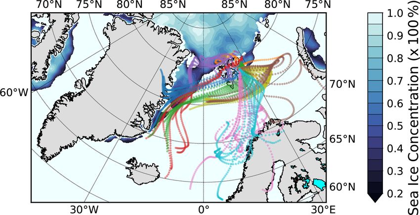
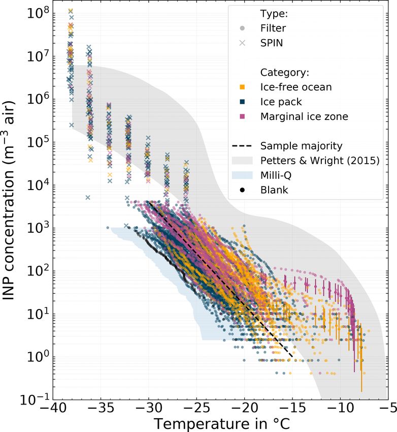
11618                                                                               M. Hartmann et al.: Terrestrial or Marine

were measured inside a temperature-controlled measurement              Na+ and Cl− mass concentrations on size-resolved am-
container located on the monkey island of the RV Polarstern.        bient aerosol particles were measured from five-stage Berner
The temperature inside the container was held at ca. 24 ◦ C,        impactor samples (mounted outside of the measurement con-
while the aerosol inlet was heated to 30 ◦ C to prevent icing.      tainer; the setup is described in detail in Kecorius et al., 2019)
The aerosol inlet consists of a 6 m long stainless-steel tub-       by ion chromatography (ICS3000, Dionex, Sunnyvale, CA,
ing (inner diameter of 40 mm), which faces upwards at a 45◦         USA), as described in Müller et al. (2010) in more detail. Ion
angle to the bow of the ship. The flow through the inlet was        chromatography was also used to determine the salinity of
set to 40 L min−1 (Reynolds number < 2000). With an isoki-          the seawater samples.
netic splitter, the aerosol was distributed between the differ-        5 d air mass back-trajectories were calculated using the
ent instruments. The aerosol instrumentation relevant to this       HYbrid Single-Particle Lagrangian Integrated Trajectory
study included a mobility particle size spectrometer (MPSS)         (HYSPLIT) model (Rolph et al., 2017; Stein et al., 2015).
to measure particle number size distributions (PNSDs), a            As input for the model, the GDAS1 meteorological fields
condensation particle counter (CPC) to measure total par-           (Global Data Assimilation System; 1◦ latitude/longitude; 3-
ticle concentration (Ntot ), and a cloud condensation nuclei        hourly) were used. Trajectories were initiated at 50, 250, and
counter (CCNC) to measure the concentrations of cloud con-          1000 m every hour.
densation nuclei (NCCN ).                                              The sea ice concentration at the position of Polarstern was
   PNSDs in the size range between 10 and 800 nm were               determined with the sea ice concentration product of the EU-
measured with a TROPOS-type MPSS (Wiedensohler et al.,              METSAT Ocean and Sea Ice Satellite Application Facility
2012). The time resolution of an upscan and downscan was            (OSI-401-b: SSMIS Sea Ice Concentration Maps on 10 km
5 min. PNSDs were derived with the inversion algorithm by           Polar Stereographic Grid; Tonboe et al., 2017).
Pfeifer et al. (2014) and corrected for transmission losses as         Chlorophyll a (Chl a) concentration was derived from the
well as counting efficiencies according to Wiedensohler et al.      vessel’s FerryBox system (4H-FerryBox, Jena Engineering,
(1997). The sizing of the MPSS was calibrated according to          Jena, Germany). A FerryBox is an autonomous online instru-
Wiedensohler et al. (2018) at regular time intervals during         ment with modular sensor assembly to continuously mea-
the campaign (for further details on the MPSS and the mea-          sure oceanographic parameters in a flow-through system (Pe-
surement container, we refer the reader to Kecorius et al.,         tersen et al., 2011, 2007). The data from the Chl a sensor
2019). Ntot was measured with a CPC (model 3010, TSI Inc.,          in the FerryBox system were accessed via the DSHIP por-
Shoreview, USA; lower cutoff: 10 nm). A CCNC (CCN-100,              tal (https://dship.awi.de/, last access: 26 March 2021) pro-
DMT, Boulder USA; Roberts and Nenes, 2005) was used to              vided by the operator of the vessel. Chl a concentrations were
measure NCCN at six different supersaturation values (SS:           also derived from satellite remote sensing (Aqua MODIS,
0.1 %, 0.15 %, 0.2 %, 0.3 %, 0.5 %, 1 %,). Each SS level was        NPP, L3SMI, Global, 4 km, Science Quality, 2003–present,
sampled for 10 min and averaged over that period; hence, a          8 d composite, 8 to 16 July).
certain SS has a time resolution of 1 h. The instrument was
calibrated with ammonium sulfate particles before and after
the campaign according to the ACTRIS protocol (Gysel and            3     Results and discussion
Stratmann, 2013).
   In addition to the offline INP analysis of the filter samples,   3.1    Atmospheric INP concentrations NINP
also the SPectrometer for Ice Nuclei (SPIN; Droplet Mea-
surements Techniques, Boulder, CO, USA) was deployed                A time series of atmospheric NINP at selected temperatures
to measure NINP in immersion mode online. SPIN is a                 derived from filter samples and online measurements with
continuous-flow diffusion chamber (CFDC) with a parallel            SPIN is shown in Fig. 2. The colored areas mark the pe-
plate geometry, and the measurement principle of SPIN in            riods when Polarstern was located in a certain environ-
immersion mode can be briefly described as follows: aerosol         ment (yellow = ice-free ocean; blue = within ice pack; pur-
particles are activated to cloud droplets and then exposed to       ple = marginal ice zone). Overall NINP is the highest at the
conditions where ice can form. The number of formed ice             beginning of the campaign, in between both legs at the harbor
crystals is then optically detected. SPIN is described in detail    of Longyearbyen, and upon entering the ice-free ocean again
in Garimella et al. (2016). SPIN was placed within a mea-           towards the end of the second leg. The lowest concentrations
surement container. Together with the other aerosol instru-         occurred when the vessel was within the ice pack. It can also
mentation, the aerosol was fed to SPIN through one main             be seen that, at a given time, peaks appear or disappear de-
inlet but with additional subsequent drying of the aerosol.         pending on temperature, indicating that different populations
SPIN sampled in half-hourly intervals of constant tempera-          of INPs contribute at warmer or colder temperatures.
ture and relative humidity, and each sampling condition was            Figure 3 shows the NINP freezing spectra for the atmo-
repeated three times within 24 h. The SPIN dataset is also          spheric filter samples measured with LINA (circle markers),
part of the overview of global shipborne INP measurements           as well as NINP (T ) measured with SPIN (cross markers).
by Welti et al. (2020).                                             The color represents the environment in which the sampling

Atmos. Chem. Phys., 21, 11613–11636, 2021                                            https://doi.org/10.5194/acp-21-11613-2021
M. Hartmann et al.: Terrestrial or Marine                                                                                            11619

Figure 2. Time series of atmospheric NINP at different temperature derived from filter samples with LINA (−22 ◦ C and above) and SPIN
measurements (−26 ◦ C and below). The bottom panel contains markers for the sample collection times of the SML, BSW, and fog water
samples. The shaded areas indicate the environment that the vessel is located in (yellow = ice-free ocean; blue = within ice pack; pur-
ple = marginal ice zone). The dark gray area indicates the period of the case study discussed in Sect. 3.5. Note that SPIN measurements were
only obtained beginning with 31 May.

https://doi.org/10.5194/acp-21-11613-2021                                               Atmos. Chem. Phys., 21, 11613–11636, 2021
11620                                                                                     M. Hartmann et al.: Terrestrial or Marine

                                                                          −10 ◦ C NINP varies between 4 × 10⁻¹ and 6 × 101 m−3 , at
                                                                          −17 ◦ C between 4 × 10⁻¹ and 1 × 10² m−3 , and at −25 ◦ C
                                                                          between 3 × 101 and 2 × 10³ m−3 . It can be seen that the
                                                                          majority of the samples are clustered around a line ranging
                                                                          roughly from 1 m−3 at −15 ◦ C to 4 × 10³ m−3 at −30 ◦ C.
                                                                          But also highly ice-active filter samples featuring NINP as
                                                                          high as 6 × 101 m−3 at −10 ◦ C were observed. These tend
                                                                          to be associated more often with the MIZ (purple symbols)
                                                                          and at −15 ◦ C also with the ice-free ocean (yellow symbols)
                                                                          environment than with the ice pack (see Fig. S10 in the Sup-
                                                                          plement). We will describe these highly ice-active samples
                                                                          in more detail in Sect. 3.5. In comparison to the range of
                                                                          NINP from midlatitudes by Petters and Wright (2015), the
                                                                          filter-derived NINP levels are lower for temperatures below
                                                                          ca. −20 ◦ C, but similar at warmer temperatures. For a given
                                                                          temperature, NINP measured with SPIN falls within the lower
                                                                          half of the NINP range by Petters and Wright (2015), with the
                                                                          exception of the two lowest temperature steps.
                                                                              In Fig. 3 it can be seen that some LINA freezing spectra
                                                                          go up to higher values (4 × 10³ m−3 ) than others (ending at
                                                                          1×10³ m−3 ). The cause of this lies in the measurement prin-
                                                                          ciple itself: DFAs only measure NINP per volume of water
                                                                          in a certain concentration range determined by the specific
Figure 3. All cumulative INP spectra derived from atmospheric             setup configuration. With the known volume of air sampled
filter samples measured with LINA (circle marker), as well as             onto one filter, these concentrations per volume of water are
NINP (T ) measured with SPIN (cross marker). The color code refers        then scaled to atmospheric concentrations per volume of air.
to the environment the sample was taken from (yellow = ice-free           Hence differing ranges of resulting values are caused by sys-
ocean; blue = ice pack; purple = marginal ice zone). The majority
                                                                          tematic differences in Vair . In our case we collected samples
of the filter samples are clustered around a line which is shown as
a black dashed line. The range of NINP for midlatitudes by Petters
                                                                          for 8 or 2 h, and since the flow rate is relatively constant, Vair
and Wright (2015) is shown as a gray shaded area for reference. The       of the 8 h samples is about 4 times larger than that of the 2 h
blue areas depicts the 10th to 90th percentile range of all pure Milli-   samples, which causes also the different reported ranges in
Q measurements with LINA (scaled to atmospheric concentrations            atmospheric NINP as seen in Fig. 3. It should also be men-
with the average sampled air volume of the 8 h samples).                  tioned that the upper and lower ends of the freezing spectra
                                                                          shown in this work only represent the limits of our detectable
                                                                          range and do not imply that outside these limits no higher
took place, based on the sea ice concentrations at the location           NINP or lower NINP existed.
of Polarstern (yellow = ice-free ocean; blue = ice pack; pur-                 The test for heat-labile INPs (Figs. S6 and S7 in the Sup-
ple = marginal ice zone, MIZ). The MIZ is defined as the                  plement) demonstrates that ice activity of the samples is re-
transitional zone between open sea and dense drift ice. It                duced when heated for 1 h at 95 ◦ C. Especially INPs that nu-
spans from 15 % to 80 % of the sea surface being covered                  cleated ice at temperatures above ca. −16 ◦ C are gone after
with ice. The area north of the MIZ is classified as the ice              the heating. This is widely seen as an indicator for the pres-
pack, and the area south of the MIZ is classified as ice-free             ence of biogenic, proteinaceous INPs as those become de-
ocean. As the filter samples were collected over the course               natured during the heating, which reduces their ice activity
of several hours on an often moving vessel, the sample en-                (Conen et al., 2011, 2012, 2017; Conen and Yakutin, 2018;
vironment might change during sampling. In such cases the                 Felgitsch et al., 2018; Hara et al., 2016; Joly et al., 2014;
sample was labeled according to the environment, which ac-                Moffett et al., 2018; Hill et al., 2016; Huang et al., 2021;
counts for most of the sampling time. The range of NINP for               McCluskey et al., 2018b; Kunert et al., 2019; Pouleur et al.,
midlatitudes by Petters and Wright (2015) is shown as a gray              1992).
shaded area for reference. Additionally, Fig. S10 in the Sup-                 In the previous section we described that at warmer tem-
plement shows a box plot of the very same filter samples, in              peratures, e.g., at −10 ◦ C, samples with high INP concentra-
order to emphasize the general differences between the envi-              tions are found more often in the MIZ and less frequently
ronments.                                                                 within the ice pack. In comparison, at the lower temperatures
   At any particular temperature, NINP varies between 2 to                measured with SPIN (cross markers in Fig. 4) no correla-
3 orders of magnitude. The variability tends to be higher                 tion with the environmental setting is found. However, in a
at warmer temperatures compared to colder temperatures: at                global context the level of NINP at these low temperatures is

Atmos. Chem. Phys., 21, 11613–11636, 2021                                                  https://doi.org/10.5194/acp-21-11613-2021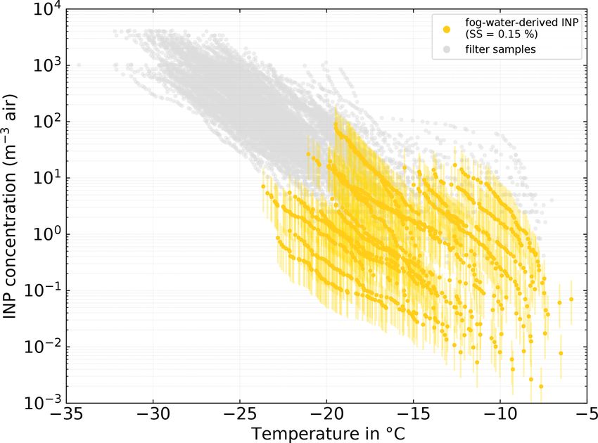
M. Hartmann et al.: Terrestrial or Marine 11621
possibly mineral dust, contribute to NINP at low temperatures
during the campaign.
3.2 INPs in sea surface microlayer and bulk seawater
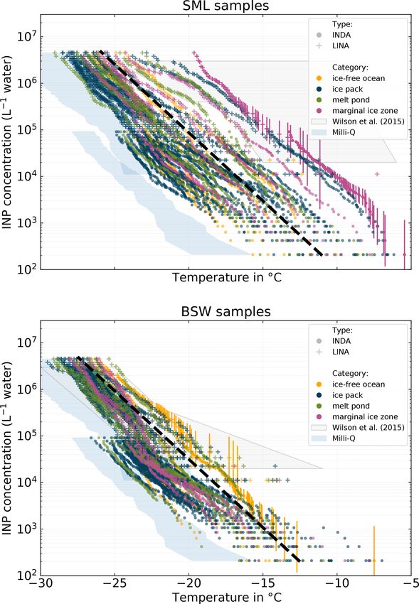
Figure 5 shows NINP per volume of water in SML and BSW.
Again, the color code refers to the environment the sample
was taken from (yellow = ice-free ocean; blue = ice pack;
purple = MIZ; green = melt point). The gray box indicates
the range of values reported in an earlier study by Wilson
et al. (2015) in the Arctic, although they did not separate their
samples into different environments. Additionally, Figs. S11
and S12 in the Supplement show box plots of the very same
SML and BSW samples in order to emphasize the general
differences between the environments.
Both SML and BSW show a high intersample variability.
Concentrations for both vary at least between 2 and 3 or-
ders of magnitude at any temperature. Some samples initiate
freezing clearly above −10 ◦ C (highest observed freezing on-
set was at −5.5 ◦ C), while for other samples freezing starts
only at temperatures below −15 ◦ C.
It is worth mentioning that the concentration range of INPs
Figure 4. Map with color-coded NINP in the Arctic at −32 ◦ C mea-
reported by Wilson et al. (2015) is not directly comparable
sured with SPIN during PS106 and also SPIN data of a transect to the measurements we present, because due to a different
from Bremerhaven (Germany) to Cape Town (South Africa) along measurement setup, they have different limits of their de-
the western coast of Africa (Welti et al., 2020). tectable range. Nevertheless, it can be seen that their SML
samples contain up to 2 orders of magnitude higher con-
centrations of INPs that are ice active at high temperatures
remarkable by itself as shown in Fig. 4. That figure shows (above ca. −10 ◦ C).
NINP in the Arctic at −32 ◦ C measured with SPIN during Interestingly, some of our samples stand out, i.e., feature
PS106 but also SPIN data by Welti et al. (2020) of a transect significantly higher ice activities at a certain temperature than
from Bremerhaven (Germany) to Cape Town (South Africa) the majority of the samples (see Fig. 5). The dashed black
along the western coast of Africa. It is striking that at these line in Fig. 5 roughly separates the samples into those that
low temperatures NINP levels in the Arctic are in the same stand out (above the line) and the rest of the very similar
order of magnitude as in the outflow region of mineral dust samples (below the line). It is noticeable that SML samples
from the Sahara. While we have no means of proving the from the known biologically active MIZ belong mostly to the
presence of mineral dust at these colder temperatures during group of samples that stand out from the rest. Also the overall
PASCAL, to our knowledge there are also no other known most active SML sample originates from the MIZ, and its
sources of INP that can produce such high concentrations connection to the corresponding atmospheric filter samples
throughout the whole time period of the campaign. Also, is discussed in more detail in the case study in Sect. 3.5. The
it was recently shown by Sanchez-Marroquin et al. (2020) high variability of the INP concentrations in SML and BSW
that Iceland can be a strong Arctic dust source. Also Irish in our view is a clear hint towards the sporadic occurrence of
et al. (2019a) suggested that observed INPs were mineral INPs in these compartments.
dust particles originating in the Arctic (Hudson Bay, eastern The SML has been found to be enriched in particulate or-
Greenland, northwest continental Canada) rather than parti- ganic matter and surface-active substances compared to the
cles originating from sea spray. And global model transport underlying bulk seawater, with enrichment factors (EFs) of
simulations done by Groot Zwaaftink et al. (2016) show that up to 10 and 50, respectively, being reported (Engel et al.,
mineral dust is not only transported into the Arctic from re- 2017; Kuznetsova and Lee, 2002). And, as described in the
mote regions but also, possibly increasingly, generated in the introduction, the SML is known to be highly ice active. It is
region itself. However, it is also possible also other sources therefore an interesting question whether INPs are also en-
of mineral INPs contribute to the INP population at these riched in the SML compared to BSW and whether enrich-
temperatures. For example, diatoms represent a biogenic but ment is a general feature in all samples or if it is restricted
mineral source of INPs, as they have a cell wall made of sil- to certain situations. To answer this question, we derived
ica (Xi et al., 2021). Therefore, it is likely that mineral INPs, INP enrichment factors for the SML, based on correspond-
https://doi.org/10.5194/acp-21-11613-2021 Atmos. Chem. Phys., 21, 11613–11636, 2021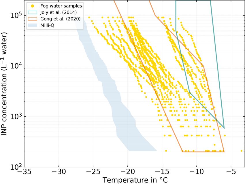
11622                                                                                   M. Hartmann et al.: Terrestrial or Marine

Figure 5. NINP in SML and BSW measured with INDA and LINA. Samples are categorized according to the environment (ice-free ocean,
ice pack, melt pond, marginal ice zone) the samples were taken from. The gray box indicates the range of values reported by Wilson et al.
(2015) for the Arctic. The blue areas depicts the 10th to 90th percentile range of all pure Milli-Q measurements with INDA and LINA.

ing SML and BSW samples as                                             currences of higher values. The highest EF we found was
                                                                       94.97. There are seven occurrences of EF = 1 and only one
               NINP, SML (T )
EFINP (T ) =                  .                               (4)      of EF ≤ 1. This result is similar to Wilson et al. (2015), who
               NINP, BSW (T )                                          only observed enrichment and no depletion of INPs in the
Figure 6 depicts the calculated EFs at selected temperatures.          SML. On the other hand, the study by Irish et al. (2017)
We observe that the majority of SML samples are enriched               also reports few cases of INPs depletion in the SML. But,
in INPs compared to the underlying BSW. The majority of                as Gong et al. (2020) pointed out, direct comparisons of EFs
EFs fall into the range between 1 and 10, with only four oc-

Atmos. Chem. Phys., 21, 11613–11636, 2021                                               https://doi.org/10.5194/acp-21-11613-2021
M. Hartmann et al.: Terrestrial or Marine 11623
Figure 6. Enrichment factors for all pairs of SML and BSW samples (INDA measurements) divided into separate panels by their environ-
mental setting. Larger markers correspond to the pairs of samples for which either the SML or the BSW sample stands out in terms of ice
activity.
between different studies are difficult since methodological observed. At −20 ◦ C, values between 1 × 10⁴ L−1 and the
differences might be of importance. upper limit of our detectable range, 9 × 10⁴ L−1 were found.
The larger markers in Fig. 6 indicate samples where the Fourteen fog samples (63.6 % of all fog samples) have a
SML showed significantly higher ice activity compared to freezing onset above −10 ◦ C, suggesting the presence of bio-
the others, i.e., higher INP concentrations (see above). Inter- genic INPs, as mineral dust only starts to contribute to the
estingly, almost exclusively the highly ice-active SML sam- INP population at temperatures below −15 ◦ C (e.g., Murray
ples are the samples which feature the highest EFs, suggest- et al., 2012; O’Sullivan et al., 2018). The highest freezing on-
ing that enrichment could be an important factor in control- set we observed in a sample was at −3.47 ◦ C. The samples
ling SML ice activity. are divided into two groups by a clearly recognizable gap.
Filtrations of 10 randomly selected SML and 12 BSW The occurrence of these two groups could not directly be re-
samples were created and analyzed for NINP to find indi- lated to meteorological parameters. However, as will be dis-
cations concerning the size of the INPs present in the sam- cussed in Sect. 3.3.1, the group of more ice-active fog sam-
ples. The samples were filtered with 0.2 µm PTFE syringe ples may be associated with the more ice-active atmospheric
filters (Puradisc 25, Whatman). While the individual sample filter samples.
was chosen randomly, it was ensured that all sample envi- In general the fog samples tend to be more ice active and
ronments (ice-free ocean, ice pack, melt pond, marginal ice show higher NINP at a given temperature than the seawater
zone) were considered. Figure 7 shows a scatter plot of the samples presented in Sect. 3.2. A qualitatively similar ob-
T10 values, i.e., the temperature where 10 % of the droplets servation was already made by Schnell (1977). For seawater
are frozen, of the filtered and unfiltered samples. If a sam- samples that they collected near Nova Scotia (Canada), they
ple falls below the 1 : 1 line, it indicates that the filtration found that some of the samples were very ice active, although
reduced the ice activity, and the distance to the 1 : 1 line in the majority of their seawater samples contained no INPs ac-
the x direction is a measure of how strong the reduction in tive at temperatures warmer than −14 ◦ C. On the other hand,
ice activity is. The complementary plots of the T50 and T90 half of their fog water samples were ice active at tempera-
can be found in the Supplement. Throughout all samples a re- tures above −10 ◦ C with the most ice-active sample initiat-
duction of the freezing temperatures can be seen due to filtra- ing freezing at −2 ◦ C. Schnell (1977) also described that they
tions. Also, the more ice active the unfiltered sample was, the found NINP in seawater, fog, and air to vary independently
larger the shift towards lower temperatures tends to be (see from each other. An observation that also largely applies to
also Fig. S4 in the Supplement). The most ice-active sample this study, but a more detailed investigation of the relation
shifted by around 5 ◦ C, while those with lower initial ice ac- between NINP in the different compartments is presented in
tivity only are decreased by approximately 2 ◦ C. This clearly the following Sect. 3.3.1 and 3.4.
indicates that a high fraction of the INPs are larger or at least The NINP (T ) we observed in Arctic fog water is similar to
associated with particles larger than 0.2 µm. what Gong et al. (2020) found in cloud water samples on the
Cabo Verde islands but tends to be lower than what was ob-
3.3 INPs in fog water served by Joly et al. (2014), who measured at Puy-de-Dôme
(France) and reported a correlation between high concentra-
Analogous to the SML and BSW samples, NINP was also de- tions of biological particles and INP concentrations. How-
termined in collected fog water samples. At −10 ◦ C, we find ever the freezing onset temperature of around −6 ◦ C is al-
NINP between the lower limit of our detectable range of 2 × most identical in the three studies.
102 and 2 × 10⁴ L−1 . At −15 ◦ C, NINP between 6 × 10² L−1
and the upper limit of our detectable range 9 × 10⁴ L−1 were
https://doi.org/10.5194/acp-21-11613-2021 Atmos. Chem. Phys., 21, 11613–11636, 202111624 M. Hartmann et al.: Terrestrial or Marine
Figure 7. Comparison of filtered and unfiltered SML and BSW samples measured with INDA. Shown are the T10 values for corresponding
samples. Symbols below the 1 : 1 line indicate that the filtered sample is less ice active.
Figure 8. NINP in fog water samples measured with INDA. The Figure 9. Fog-water-derived NINP in air. NINP was derived from
teal and orange polygons show the range of values observed by Joly Eqs. (5) and (6) with the median NCCN (SS = 0.15 %) during the
et al. (2014) and Gong et al. (2020), respectively. time of each fog sample and an average droplet diameter (ddrop ) of
17 µm. The error bars show the range with ddrop of 12 and 22 µm,
respectively. See Sect. 3.3.1 for details on the derivation method.
3.3.1 Connecting INPs in clear or fog-free air to fog
samples
In this section we relate and compare NINP in fog water sam- typically low (0.02 %–0.2 %; Pruppacher and Klett, 2010).
ples with those measured in fog-free air (see Sect. 3.1), fol- Thus we choose NCCN measured at SS = 0.15 % as a proxy
lowing the procedure introduced in Gong et al. (2020), which for the droplet number concentration. Please note that we do
is briefly described in the following. The number concentra- not use NCCN measured at SS = 0.1 %, because after the re-
tion of CCN (NCCN ) at a particular supersaturation (SS) is moval of data points due to quality assurance, the data cov-
used as a proxy for the fog droplet number concentration. erage for SS = 0.15 % is significantly better than for SS =
Furthermore, Gong et al. (2020) made the legitimate assump- 0.1 %.
tion, that all INPs act as CCN. Together with an estimated fog Remote sensing studies of Arctic cloud droplet sizes report
droplet diameter (ddrop ), the volume of fog water per volume typical diameters between 14 and 20 µm (Bierwirth et al.,
dry air, LWCfog , can be calculated as follows: 2013; Shupe et al., 2001; King et al., 2004) and in situ ob-
servations found values between 12 and 22 µm. Hence we
3 use 17 µm as an average ddrop and vary it between 12 and
LWCfog = NCCN · π/6 · ddrop . (5)
22 µm. With that we calculate a range of LWCfog , which is
For determining NCCN , a SS needs to be defined. Since fog, then further used to derive the INP number concentration in
unlike clouds, is characterized by low updrafts, SS is also air, NINP, air , based on the INP concentration in fog water,
Atmos. Chem. Phys., 21, 11613–11636, 2021 https://doi.org/10.5194/acp-21-11613-2021M. Hartmann et al.: Terrestrial or Marine 11625
NINP, fogwater :
NINP, air = LWCfog · NINP, fogwater . (6)
Figure 9 depicts NINP as determined from the clear-air fil-
ter samples with gray symbols and the ones derived from
the fog water samples in yellow. Overall, measured and de-
rived NINP are in good agreement. Unfortunately, as multiple
atmospheric filter samples were taken during the collection
time of a single fog sample, an unambiguous attribution of
a filter to a fog sample is difficult. Therefore, here we can
only report the half-quantitative observation that the freez-
ing spectra of the atmospheric filter samples taken concur-
rently with the most ice-active fog samples and the spectra
derived from the fog water samples feature similar shapes,
with the shapes themselves and the onset of freezing at tem-
peratures above −10 ◦ C suggesting the presence of biogenic
INPs. This clearly points at the same or at least similar, partly
biogenic, INP populations being present in both fog droplets
and atmospheric aerosol particles. Also Gong et al. (2020)
found general agreement between NINP in the air and NINP
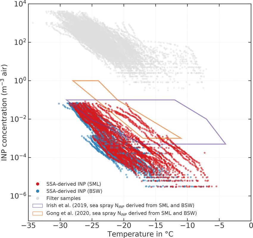
Figure 10. Sea-spray-derived atmospheric NINP (red sym-
derived from, in their case, cloud water samples. They further
bols = derived from SML samples; blue symbols = derived from
observed that highly ice-active particles are activated into BSW samples; measurements with INDA and LINA). The gray
cloud droplets during cloud events and then can be found symbols show the filter-derived atmospheric NINP . The orange and
in the cloud water. It is likely that a similar process occurs purple polygons indicate the range of sea spray aerosol (SSA)-
during our fog events. derived NINP by Irish et al. (2019b) and Gong et al. (2020), re-
It should be noted that if NCCN changes significantly dur- spectively. Samples from melt ponds are excluded.
ing the sampling time of the respective fog sample, the fog-
derived atmospheric NINP is directly affected. Such an in-
stance can be seen in the lowest fog-derived INP spectra amount of NaCl present in the seawater as a scaling factor
seawater into atmospheric N
to translate NINP
in Fig. 9, where the low average NCCN led to a deviation INP . In this simple
of around 1 order of magnitude in comparison to the atmo- model, no enrichment of INPs is accounted for in the course
spheric sample. In the Supplement (Sect. S9), the fog-water- of sea spray
production. The sea-spray-derived INP concen-
seaspray, air
derived NINP levels are shown for an extrapolated value of trations NINP are calculated as
NCCN at SS = 0.02 %. With that value, the agreement be-
tween the filter- and fog-derived NINP is reduced; neverthe- seaspray, air NaClmass, air seawater
NINP = · NINP , (7)
less, both still overlap by 1 to almost 2 orders of magnitude. NaClmass, seawater
A linear extrapolation to such low supersaturations has large where NaClmass, air and NaClseawater are the mass concentra-
uncertainties; hence, it should be only seen as an estimate tions of sodium chloride in corresponding air and seawa-
for the lower boundary of the presented derivation method of ter samples, respectively. NaClmass,air varied between 0.04
NINP in air from fog water samples. and 1.9 µg m−3 during the campaign with an average of
0.48 µg m−3 . The average NaClseawater of all SML and BSW
3.4 Connecting atmospheric INPs to sea spray
samples is 32.5 g L−1 with actual concentrations varying be-
In order to assess the ocean as a possible source of atmo- tween 25.7 and 34.5 g L−1 . NaClseawater was derived from the
spheric INPs, we derive potential atmospheric NINP by vir- salinity of the samples with the simplifying assumption that
tually dispersing the characterized seawater samples as sea NaCl is the only salt in the sea water. This assumption is jus-
spray (Irish et al., 2019b; Gong et al., 2020). This thought tified as non-NaCl salts represent only minor constituents of
experiment can be paraphrased as follows: if the seawater the sea water. Samples from melt ponds are excluded here
samples including all their INPs would be directly dispersed and also in the following as they are mostly fresh water and
into the air, scaled by the measured relation between salt in therefore not suited for this approach that is based on NaCl
the air and in the water, what would be the resulting NINP in concentration.
the air? Figure 10 shows atmospheric filter-derived NINP in gray
seaspray, air
For this approach, we use the amount of NaCl present and the sea-spray-derived NINP (red symbols corre-
in the atmospheric aerosol particles (derived from chemi- spond to SML samples and blue ones to BSW samples). As
seaspray, air
cal analysis of Berner impactor samples) in relation to the can be seen, NINP falls mostly in the range between
https://doi.org/10.5194/acp-21-11613-2021 Atmos. Chem. Phys., 21, 11613–11636, 202111626 M. Hartmann et al.: Terrestrial or Marine
10−6 and 10−1 m−3 , which is approximately 3 to 5 orders
of magnitude lower than the atmospheric NINP derived from
our atmospheric filter samples. Our lower end of the de-
rived concentration range (10−6 m−3 ) is also roughly 3 or-
ders of magnitude lower than the lower end of the range
reported by Gong et al. (2020), who sampled near the sub-
tropical islands of Cabo Verde during late summer, and Irish
et al. (2019b), who measured in the Canadian Arctic during
early summer. These differences could be due to the geo-
graphical settings of the samples being vastly different, even
for the Arctic measurements by Irish et al. (2019b). Irish
et al. (2019b) took samples comparatively close to the shore
mainly in the Nares Strait and Baffin Bay during summer
with no extensive sea ice cover present, whereas we sampled
mostly within the ice pack hundreds of nautical miles away
from bigger lands masses. But even if the ranges given in
Gong et al. (2020) and Irish et al. (2019b) are considered,
our atmospheric filter-derived NINP levels are still orders of
magnitude higher than any sea-spray-derived NINP . This in-
dicates that sea spray aerosol as a sole source is not suffi-
cient to explain atmospheric NINP without significant enrich-
ment of INPs during sea spray production. To the authors’
knowledge, there are no studies available on the enrichment
of INPs in sea spray aerosol (SSA). However, studies about
the enrichment of bacteria and organic matter exist. Blan-
chard (1978) describes that in jet drops, which are produced
when bubbles burst at the air–water interface, bacteria can
get enriched by a factor greater than 103 . While several fac-
tors, including the type of bacteria themselves, control the
EF of bacteria, the findings by Blanchard (1978) suggest that
Figure 11. (a) Filter samples measured with LINA. Samples that
similar EFs may also apply to INP, since bacteria are a ma-
were collected during the period of the case study are shown in
jor contributor to seawater ice activity, as described in the
color, while all other samples are shown in gray. Exemplary fits for
introduction. For organic matter, EFs of 104 to 105 (in rela- the slopes at lower and higher temperatures for case-study-related
tion to mass) are reported for submicron SSA (Keene et al., samples are shown as orange and blue lines, respectively. The black
2007; Van Pinxteren et al., 2017) and 102 for supermicron dots depict the mean freezing spectrum of the field blanks scaled
SSA (Quinn et al., 2015; Keene et al., 2007). As we have to atmospheric concentrations with the mean sampled air volume
no information about the size of the INPs, except that they of the 8 h filter samples. (b) SML samples measured with INDA.
are larger than 0.2 µm, we cannot say what enrichment factor The sample that was collected during the period of the case study
would be an appropriate assumption in regard to INPs, but is shown in color, while all other samples are shown in gray. As in
the abovementioned literature indicates that processes exist (a), the fits of the slope are shown as orange and blue lines.
that can produce sufficiently high enrichment factors at least
for some substance classes. But it should be also noted that
the laboratory study by Ickes et al. (2020) did not find a cor- 3.5 Case study
relation between total organic carbon content of algal culture
In Sect. 3.1, we described that INP concentrations are dif-
samples and the freezing of the sample. The same study con-
ferent in the ice-free ocean, within the ice pack, and close
firmed that the transfer of ice-nucleating material from the
to land. In the following we will show that merely the prox-
seawater to the aerosol phase can indeed happen. Therefore,
imity to land does not make marine INP sources inferior to
a marine source for the INPs in the Arctic atmosphere can-
terrestrial ones. To elucidate this, we consider a time period
not be ruled out, but considerable enrichment of INPs during
of several filter-sampling intervals which occurred around a
the transfer from the ocean surface to the atmosphere would
time when both atmospheric and INP concentrations in the
have to take place.
SML were highest. This happened close to Svalbard and in
the vicinity of the ice edge, which makes the situation even
more interesting.
Atmos. Chem. Phys., 21, 11613–11636, 2021 https://doi.org/10.5194/acp-21-11613-2021You can also read