Glacier algae accelerate melt rates on the south-western Greenland Ice Sheet - GFZpublic
←
→
Page content transcription
If your browser does not render page correctly, please read the page content below
The Cryosphere, 14, 309–330, 2020
https://doi.org/10.5194/tc-14-309-2020
© Author(s) 2020. This work is distributed under
the Creative Commons Attribution 4.0 License.

Glacier algae accelerate melt rates on the south-western
Greenland Ice Sheet
Joseph M. Cook1,2 , Andrew J. Tedstone3 , Christopher Williamson4 , Jenine McCutcheon5 , Andrew J. Hodson6,7 ,
Archana Dayal1,6 , McKenzie Skiles8 , Stefan Hofer3 , Robert Bryant1 , Owen McAree9 , Andrew McGonigle1,10 ,
Jonathan Ryan12 , Alexandre M. Anesio13 , Tristram D. L. Irvine-Fynn11 , Alun Hubbard14 , Edward Hanna15 ,
Mark Flanner16 , Sathish Mayanna17 , Liane G. Benning5,17,18 , Dirk van As19 , Marian Yallop4 , James B. McQuaid5 ,
Thomas Gribbin3 , and Martyn Tranter3
1 Department    of Geography, University of Sheffield, Winter Street, Sheffield, South Yorkshire, S10 2TN, UK
2 Institute of Biological, Environmental and Rural Sciences, Aberystwyth University, Aberystwyth, SY23 3DA, UK
3 Bristol Glaciology Centre, School of Geographical Sciences, University of Bristol, Berkely Square, Bristol, BS8 1RL, UK
4 School of Biological Sciences, University of Bristol, Tyndall Ave, Bristol, BS8 1TQ, UK
5 School of Earth and Environment, University of Leeds, Leeds, LS2 9JT, UK
6 Department of Geology, University Centre in Svalbard, Longyearbyen, 9171, Norway
7 Department of Environmental Sciences, Western Norway University of Applied Sciences, 6856 Sogndal, Norway
8 Department of Geography, University of Utah, Central Campus Dr, Salt Lake City, Utah, USA
9 Faculty of Science, Liverpool John Moores University, James Parsons Building, Byrom Street, Liverpool, L3 3AF, UK
10 School of Geosciences, University of Sydney, Sydney, NSW 2006, Australia
11 Department of Geography and Earth Science, Aberystwyth University, Wales, SY23 3DB, UK
12 Institute at Brown for Environment and Society, Brown University, Providence, Rhode Island, USA
13 Department of Environmental Science, Aarhus University, 4000 Roskilde, Denmark
14 Centre for Gas Hydrate, Environment and Climate, University of Tromsø, 9010 Tromsø, Norway
15 School of Geography and Lincoln Centre for Water and Planetary Health, University of Lincoln, Think Tank, Ruston Way,

Lincoln, LN6 7DW, UK
16 Climate and Space Sciences and Engineering, University of Michigan, 2455 Hayward St. Ann Arbor, Michigan, USA
17 German Research Centre for Geosciences, GFZ, Potsdam, Germany
18 Department of Earth Sciences, University of Berlin, Berlin, Germany
19 Geological Survey of Denmark and Greenland, Copenhagen, Denmark

Correspondence: Joseph M. Cook (joc102@aber.ac.uk)

Received: 18 March 2019 – Discussion started: 3 April 2019
Revised: 16 December 2019 – Accepted: 18 December 2019 – Published: 29 January 2020

Abstract. Melting of the Greenland Ice Sheet (GrIS) is the       gal growth led to an additional 4.4–6.0 Gt of runoff from bare
largest single contributor to eustatic sea level and is ampli-   ice in the south-western sector of the GrIS in summer 2017,
fied by the growth of pigmented algae on the ice surface,        representing 10 %–13 % of the total. In localized patches
which increases solar radiation absorption. This biological      with high biomass accumulation, algae accelerated melting
albedo-reducing effect and its impact upon sea level rise has    by up to 26.15 ± 3.77 % (standard error, SE). The year 2017
not previously been quantified. Here, we combine field spec-     was a high-albedo year, so we also extended our analysis
troscopy with a radiative-transfer model, supervised clas-       to the particularly low-albedo 2016 melt season. The runoff
sification of unmanned aerial vehicle (UAV) and satellite        from the south-western bare-ice zone attributed to algae was
remote-sensing data, and runoff modelling to calculate bio-      much higher in 2016 at 8.8–12.2 Gt, although the propor-
logically driven ice surface ablation. We demonstrate that al-   tion of the total runoff contributed by algae was similar at

Published by Copernicus Publications on behalf of the European Geosciences Union.
310                                                                      J. M. Cook et al.: Glacier algae accelerate melt rates

9 %–13 %. Across a 10 000 km2 area around our field site, al-       (Wientjes et al., 2011, 2016; Tedstone et al., 2017; Stibal et
gae covered similar proportions of the exposed bare ice zone        al., 2017). There is a growing literature demonstrating the
in both years (57.99 % in 2016 and 58.89 % in 2017), but            albedo-reducing role played by a community of algae that
more of the algal ice was classed as “high biomass” in 2016         grow on glacier ice on the eastern (Lutz et al., 2014) and
(8.35 %) than 2017 (2.54 %). This interannual comparison            western (Uetake et al., 2010; Yallop et al., 2012; Stibal et al.,
demonstrates a positive feedback where more widespread,             2017; Tedstone et al., 2017; Williamson et al., 2018) GrIS.
higher-biomass algal blooms are expected to form in high-           The algal community on the GrIS is dominated by Mesotae-
melt years where the winter snowpack retreats further and           nium berggrenii and Ancylonema nordenskioldii (Yallop et
earlier, providing a larger area for bloom development and          al., 2012; Stibal et al., 2017; Williamson et al., 2018, 2019;
also enhancing the provision of nutrients and liquid water          Lutz et al., 2018), which are collectively known as “glacier
liberated from melting ice. Our analysis confirms the impor-        algae” to distinguish them from snow algae and sea ice al-
tance of this biological albedo feedback and that its omission      gae. The presence of these glacier algae reduces the albedo
from predictive models leads to the systematic underestima-         of the ice surface, mostly due to a purple purpurogallin-like
tion of Greenland’s future sea level contribution, especially       pigment (Williamson et al., 2018; Stibal et al., 2017; Remias
because both the bare-ice zones available for algal coloniza-       et al., 2012).
tion and the length of the biological growth season are set to         An equivalent albedo reduction due to algae has also
expand in the future.                                               been studied on snow. Worldwide, snow algal communities
                                                                    are dominated by unicellular Chlamydomonaceae, the most
                                                                    abundant of which belong to the collective taxon Chlamy-
                                                                    domonas nivalis (Leya et al., 2004). These algae have been
1   Introduction                                                    shown to be associated with low-albedo snow in eastern
                                                                    Greenland (Lutz et al., 2014) and to be responsible for 17 %
Mass loss from the Greenland Ice Sheet (GrIS) has increased         of snowmelt in Alaska (Ganey et al., 2017). However, for
over the past 2 decades (Shepherd et al., 2012; Hanna et al.,       glacier algae, quantification of the biological albedo reduc-
2013) and is the largest single contributor to cryospheric sea      tion, radiative forcing and melt acceleration has remained
level rise, adding 37 % or 0.69 mm yr−1 between 2012 and            elusive due to the difficulty of separating biological from
2016 (Bamber et al., 2018). This is due to enhanced surface         non-biological albedo-reducing processes and a lack of di-
melting (Ngheim et al., 2012) that exceeds calving losses at        agnostic biosignatures for remote sensing. For snow, remote
the ice sheet’s marine-terminating margins (Enderlin et al.,        detection has been achieved by measuring the “uniquely bio-
2014; van den Broeke et al., 2016). Surface melting is con-         logical” chlorophyll absorption feature at 680 nm (Painter et
trolled by net solar radiation, which in turn depends upon the      al., 2001), a broader carotenoid absorption feature (Takeuchi
albedo of the ice surface, making albedo a critical factor for      et al., 2006), a normalized difference spectral index (Ganey
modulating ice sheet mass loss (Box et al., 2012; Ryan et           et al., 2017) and a spectral unmixing model (Huovinen et
al., 2018a). The largest shift in albedo occurs when the win-       al., 2018). However, these signature spectra can be ambigu-
ter snow retreats to expose bare glacier ice. However, there        ous for glacier algae due to the presence of the phenolic pig-
are several linked mechanisms that then change the albedo of        ment with a broad range of absorption across the UV and VIS
the exposed ice and determine its rate of melting, including        wavelengths that obscures features associated with other pig-
meltwater accumulation, ice surface weathering and the ac-          ments in raw reflectance spectra and is further complicated
cumulation of light-absorbing particles (LAPs), such as soot        by the highly variable optics of the underlying ice and mix-
(Flanner et al., 2007) and mineral dust (Skiles et al., 2017).      ing of algae with other impurities.
Photosynthetic algae also reduce the albedo of the GrIS (Ue-           The dark zone is of the order 105 km2 in extent and is un-
take et al., 2010; Yallop et al., 2012; Stibal et al., 2017; Ryan   dergoing long-term expansion (Shimada et al., 2016; Ted-
et al., 2017, 2018b). Despite being identified in the late 1800s    stone et al., 2017). Quantifying the impact of algal coloniza-
(Nordenskiöld, 1875), their effects have not yet been quanti-       tion on the dark zone is therefore paramount. Upscaling of
fied, mapped or incorporated into any predictive surface mass       unmanned aerial vehicle (UAV) observations made in a small
balance models (Langen et al., 2017; Noël et al., 2016; Fet-        sector of the dark zone to satellite data has demonstrated that
tweis et al., 2017). Hence, biological growth may play an im-       “distributed impurities” including algae exert a primary con-
portant yet underappreciated role in the melting of the Green-      trol on the surface albedo, but isolating the biological effect
land Ice Sheet and its contributions to sea level rise (Benning     and upscaling to the regional scale has been prevented by
et al., 2014).                                                      a lack of spectral resolution and ground validation (Ryan et
   The snow-free surface of the GrIS has a conspicuous dark         al., 2018a). Recently, Wang et al. (2018) applied the vege-
stripe along its western margin that expands and contracts          tation red edge (difference in reflectance between 673 and
seasonally, covering 4 %–10 % of the ablating bare-ice area         709 nm) to map glacier algae over the south-western GrIS
(Shimada et al., 2016). The extent and darkness of this “dark       using Sentinel-3 OLCI data at 300 m ground resolution. Nei-
zone” may be biologically and/or geologically controlled

The Cryosphere, 14, 309–330, 2020                                                         www.the-cryosphere.net/14/309/2020/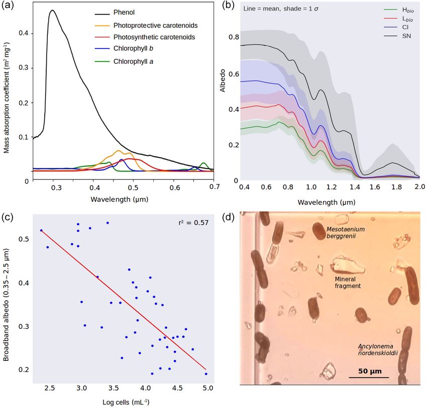
J. M. Cook et al.: Glacier algae accelerate melt rates                                                                        311

ther of these previous studies quantified the effect of glacier    algal coverage from our remote-sensing imagery and calcu-
algae effect on albedo or melt at the regional scale.              lations of the proportion of melting attributed to algae from
   Here, we directly address these issues, resolving a major       our field data, we were able to estimate runoff attributed to
knowledge gap limiting our ability to forecast ice sheet melt      algae using the runoff model by van As et al. (2017). The
rates into the future. First, we use spectroscopy to quantify      details of each stage of our methodology are provided in the
the effect of glacier algae on albedo and radiative forcing in     following Sect. 2.2–2.10.
ice. We then use a new radiative-transfer model to isolate
the effects of individual light-absorbing particles on the ice     2.2   Field site
surface for the first time, enabling a comparison between lo-
cal mineral dust and algae and providing the first candidate       Experiments were carried out at the Black and Bloom Project
albedo parameterization that could enable glacier algae to be      field site (67.04◦ N, 49.07◦ W; Fig. 1), near the Institute for
incorporated into mass balance models. To determine spa-           Marine and Atmospheric research Utrecht (IMAU) Auto-
tial coverage, we apply a supervised classification algorithm      matic Weather Station “S6” on the south-western Green-
(random forest) to map glacier algae in multispectral UAV          land Ice Sheet between 10 and 22 July 2017. We estab-
and satellite data. Runoff modelling informed by our empir-        lished a 200 × 200 m area for UAV mapping (centred on
ical measurements and remote-sensing observations enables          67.07789444◦ N, 49.350000◦ W) where only essential ac-
us to estimate the biological contribution to GrIS runoff for      cess was allowed (e.g. for placing ground control points,
the first time.                                                    GCPs, for geo-rectifying our UAV images) and sample re-
                                                                   moval was prohibited. We also delineated an additional ad-
                                                                   jacent 20 × 200 m area that we referred to as the “sampling
2     Field sites and methods                                      strip” in which we made spectral reflectance and albedo mea-
                                                                   surements paired with removal of samples for biological and
2.1    Overview                                                    mineralogical analyses, as detailed in the following sections.
                                                                   The sampling strip was subdivided into smaller subregions
In this study we present a suite of empirical, theoretical and     that were then systematically visited each day of our field
remote-sensing data to quantify and map algal contributions        season. This was necessary because ice surface samples were
to melting on the south-western GrIS. At our field site we         destructively removed for analysis and this method ensured
paired spectral reflectance and albedo measurements with re-       that each area visited had not been disturbed by our pres-
moval of surface ice samples for biological and mineralogi-        ence on previous days. Some ancillary directional reflectance
cal analyses in order to quantify the relationship between cell    measurements were also made at the same field site between
abundance and broadband and spectral albedo. The imagi-            15 and 25 July 2016 and appended to our training dataset for
nary part of the refractive index of the local mineral dusts       supervised classification (Sect. 2.8).
and the purpurogallin-type phenolic compound that domi-
nates absorption in the local glacier algae were measured in       2.3   Field spectroscopy
the laboratory and incorporated into a new radiative-transfer
model. The albedo effects of each impurity were thus ex-           At each site in our sampling strip, albedo was measured us-
amined in isolation and compared. At the same time, we             ing an ASD (Analytical Spectral Devices, Colorado) Field-
also undertook a sensitivity study with other bulk dust op-        Spec Pro 3 spectroradiometer with an ASD cosine collector.
tical properties from previous literature to further test the      The cosine collector was mounted horizontally on a 1.5 m
potential role of mineral dusts in darkening the ice surface.      crossbar levelled on a tripod with a height between 30 and
Furthermore, by combining albedo measurements with in-             50 cm above the ice surface. The cosine collector was po-
coming irradiance spectra and measurements of local melt           sitioned over a sample surface, connected to the spectrora-
rates, we estimated the radiative forcing and the proportion       diometer using an ASD fibre optic. Following this, the spec-
of melting that could be attributed to algae in areas of high      troradiometer was controlled remotely from a laptop, mean-
and low algal biomass (Hbio and Lbio ). At our field site we       ing the operators could move away from the instrument to
made UAV flights with a multispectral camera in order to           avoid shading it. Two upwards- and two downwards-looking
map algal coverage at high spatial resolution. We achieved         measurements were made in close succession (∼ 2 min) to
this by training a random-forest (RF) algorithm on our field       account for any change in atmospheric conditions, although
spectroscopy data to classify the ice surface into discrete cat-   the measurements presented were all made during constant
egories including Hbio and Lbio . This enabled estimates of        conditions of clear skies at solar noon ±2 h. Each retrieval
algal coverage in a 200 × 200 m area at our field site. We         was the average of > 20 replicates.
then retrained our classifier for Sentinel-2 satellite imagery        Immediately after making the albedo measurements, the
and used this to upscale further within the south-western re-      cosine collector was replaced with a 10◦ collimating lens,
gion of the GrIS (to a 100 × 100 km Sentinel-2 tile covering       enabling a nadir view hemispheric conical reflectance fac-
our field site and UAV image area). With these estimates of        tor (HCRF) measurement to be obtained. For HCRF mea-

www.the-cryosphere.net/14/309/2020/                                                        The Cryosphere, 14, 309–330, 2020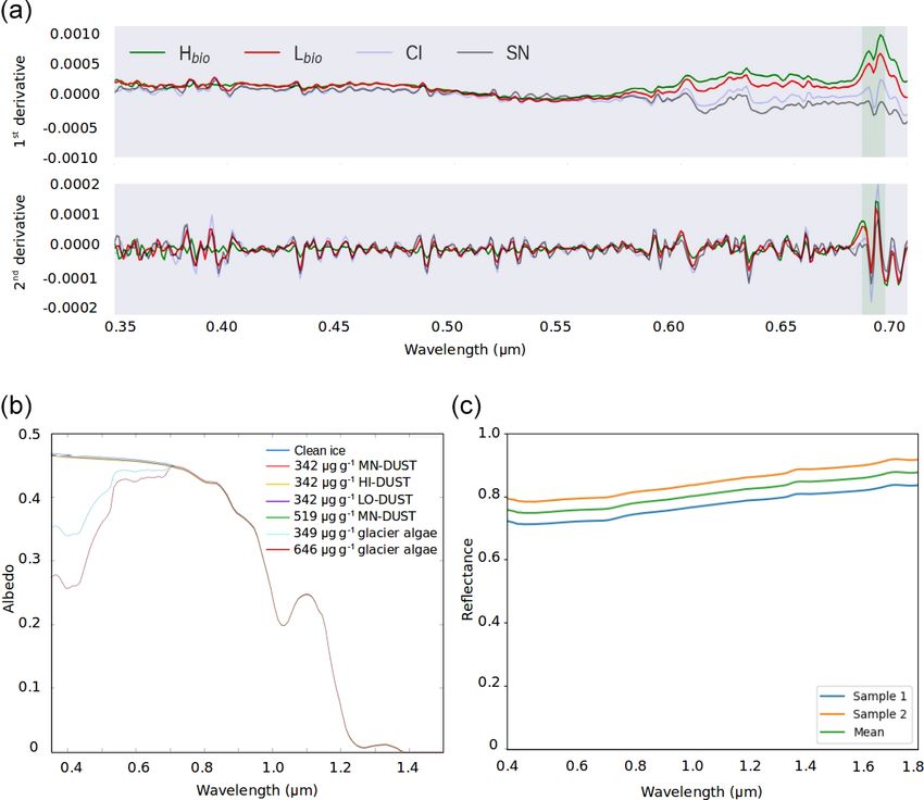
312 J. M. Cook et al.: Glacier algae accelerate melt rates
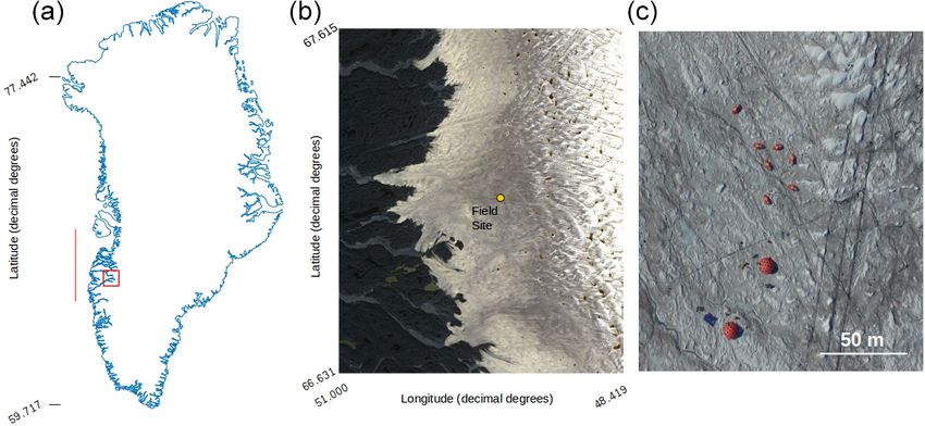
Figure 1. (a) Map of Greenland showing the bounding box of the Sentinel-2 tile (22WEV) containing our field site (red box) and the
latitudinal extent of our runoff modelling (red line). The basemap was created using the MATLAB Arctic Mapping Toolbox (Greene et al.,
2017). The Sentinel-2 tile outlined by the red box is shown in detail in (b) with the field site marked with a yellow dot. Sentinel-2 bands 2,
3 and 4 were combined into a true-colour composite using GDAL (geographical data abstraction library, 2019), by the lead author. Panel (c)
shows the area immediately surrounding the field camp as captured by a DJI Phantom Pro by the lead author.
surements the upwards-looking measurements were replaced millilitre. Biovolume was determined by measuring the long
with HCRF measurements of a flat Spectralon® panel with and short axes of at least 10 cells from each species in each
the spectroradiometer in reflectance mode. This protocol was sample using the measure tool in the GNU Image Manipu-
followed for every sample surface, with both albedo and di- lation Program (GIMP). The morphology of the cells in the
rectional reflectance measurements taking less than 5 min. images was used to separate them into two species: Mesotae-
We closely followed the methodology described by Cook et nium berggrenii and Ancylonema nordenskioldii. These di-
al. (2017b). Albedo is the most appropriate measurement for mensions were then used to calculate the mean volume of
determining the surface energy balance, while the HCRF is each species in each sample, assuming the cells to be circu-
closer to the measurements made by aerial remote sensing lar cylinders (following Hillebrand, 1999, and Williamson et
and less sensitive to stray light reflecting from surfaces other al., 2018). The average volume was multiplied by the num-
than the homogeneous patch directly beneath the sensor. We ber of cells for each species and then summed to provide the
therefore used the albedo for energy balance calculations and total biovolume for each sample.
the HCRF for remote-sensing applications in this study.
2.5 Mineral and algal optical properties and
2.4 Biological measurements
radiative-transfer modelling
Immediately following the albedo and HCRF measurements,
ice from within the viewing area of the spectrometer was re- A new radiative-transfer package, BioSNICAR_GO, was de-
moved using a sterile blade and scooped into sterile Whirl- veloped for this study and was used to predict the albedo
Pak bags, melted in the dark and immediately fixed with of snow and ice surfaces with algae and mineral dusts. We
3 % glutaraldehyde. The samples were then returned to made a series of major updates and adaptations to the BioS-
the University of Bristol and University of Sheffield where NICAR model presented by Cook et al. (2017b). The pack-
microscopic analyses were undertaken. Samples were vor- age is divided into a bio-optical scheme wherein the optical
texed thoroughly before 20 µL was pipetted into a Fuchs– properties of light-absorbing impurities and ice crystals can
Rosenthal haemocytometer. The haemocytometer was di- be calculated using Mie scattering (for small spherical parti-
vided into 4 × 4 image areas. These were used to count a cles such as black carbon or snow) or geometrical optics (for
minimum of 300 cells to ensure adequate representation of large and/or aspherical particles such as glacier algae, larger
species diversity (where possible, as some low-abundance mineral dust particles, and large ice crystals) and a two-
samples had as few as one cell per haemocytometer). The stream radiative-transfer model based on SNICAR (Flanner
volume of each image area was used to calculate cells per et al., 2007), which incorporates the equations of Toon et
The Cryosphere, 14, 309–330, 2020 www.the-cryosphere.net/14/309/2020/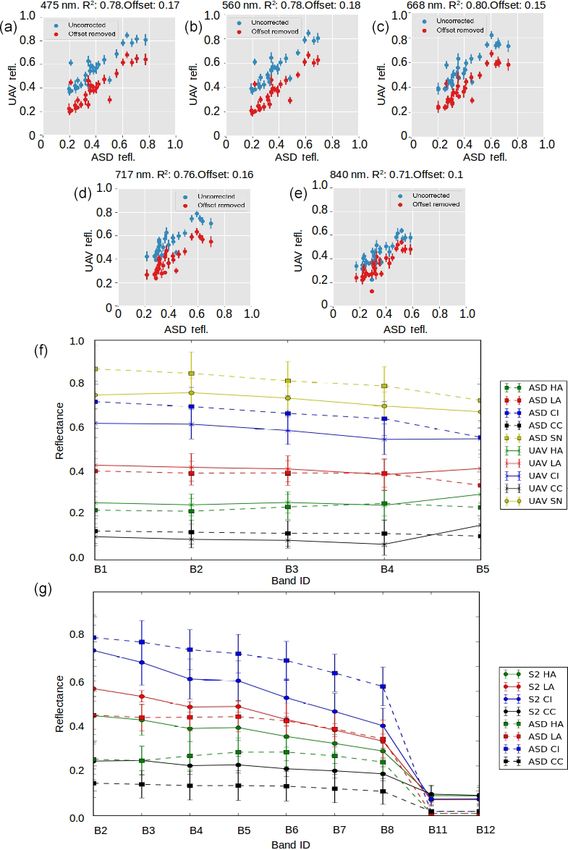
J. M. Cook et al.: Glacier algae accelerate melt rates                                                                        313

al. (1989). A schematic of the model structure is provided        mass fractions (after converting to volumetric fractions us-
in the Supplement (Sect. S1).                                     ing the mineral densities), generated the single-scattering
   To incorporate glacier algae into BioSNICAR_GO, ge-            optical properties using a Mie scattering code and applied
ometrical optics were employed to determine the single-           a weighted average using the PSD to obtain the bulk opti-
scattering optical properties of the glacier algae, since they    cal properties for the dust. Since the mineralogy of the dust
are large (∼ 103 µm3 , making Mie calculations impractically      varied between sites we generated three dust “scenarios”.
computationally expensive) and best approximated as circu-        In the low-absorption scenario (LO-DUST) all the minerals
lar cylinders (Hillebrand, 1999; Lee and Pilon, 2003). Our        were set to the minimum volume-fraction measured across
approach is adapted from the geometric optics parameteriza-       all of McC’s samples except for quartz, which comprised the
tion of van Diedenhoven (2014). The inputs to the geomet-         remainder. In the high-absorption scenario (HI-DUST) all
ric optics calculations are the cell dimensions and the com-      the minerals were set to their maximum measured volume-
plex refractive index. The imaginary part of the refractive in-   fraction, apart from quartz, which comprised the remainder.
dex was calculated using a mixing model based upon Cook           Finally, in the mean scenario (MN-DUST) all the minerals
et al. (2017b), where the absolute mass of each pigment in        were present with their volume fractions equal to the mean
the algal cells was measured in field samples. The absorp-        across all of the field samples. The mineralogy of each of
tion spectra for the algal pigments is provided in Fig. 2a.       these scenarios is described in Table 1. Refractive indices
We updated the mixing model by Cook et al. (2017b) to ap-         were not available for all of the individual minerals present
ply a volume-weighted average of the imaginary part of the        in McC’s analysis, so we represented the feldspar minerals
refractive index of water and the algal pigments so that the      using the refractive index for andesite (Pollack et al., 1973)
simulated cell looks like water at wavelengths where pig-         and all pyroxenes with the refractive index for enstatite (Jäger
ments are non-absorbing. We consider this to be more phys-        et al., 2003), and, in the absence of a refractive index for
ically realistic than having cells that are completely non-       amphibole phases, we used the refractive index for the simi-
absorbing at wavelengths > 0.75 µm, especially since a wa-        larly green mineral olivine (OCDB, 2002). Refractive indices
ter fraction (Xw ) is used in the calculations to represent the   for all other minerals were available (Rothman et al., 1998;
non-pigmented cellular components of the total cell volume.       Roush et al., 1991; Pollack et al., 1973; Egan and Hilgeman,
This approach also prevents the refractive index from be-         1983; Nitsche and Fritz, 2004).
coming infinite when the water fraction is zero, removing            The ice optical properties in BioSNICAR-GO were also
the constraint 0 < Xw < 1 from the bio-optical scheme in          calculated using a parameterization of geometric optics
the original BioSNICAR model. Based upon experimental             adapted from van Diedenhoven et al. (2014). A geometri-
evidence in Dauchet et al. (2015) for the model species C.        cal optics approach to generating ice optical properties was
reinhardii, the real part of the refractive index has been up-    chosen because it enables arbitrarily large ice grains with
dated from 1.5 (in Cook et al., 2017b) to 1.4. The absorp-        a hexagonal columnar shape to be simulated, in order to
tion coefficients from which the imaginary refractive index       better estimate the albedo of glacier ice where grains are
is calculated are from Dauchet et al. (2015), apart from the      large and aspherical. While the real ice surface is composed
purpurogallin-type phenol, whose optical properties were de-      of irregularly shaped and sized grains, this approach en-
termined empirically (Fig. 2a). The calculated optical prop-      abled us to simulate our field spectra much more accurately
erties were added to the lookup library for BioSNICAR-GO          and circumvented the requirements that individual grains be
for a range of cell dimensions. For the simulations presented     small and spherical in the case of the Lorenz–Mie approach.
in this study, we included two classes of glacier algae rep-      The optical properties of the ice grains were modelled us-
resenting Mesotaenium berggrenii and Ancylonema norden-           ing refractive indices from Warren and Brandt (2008). The
skioldii with length and diameter and also the relative abun-     radiative-transfer model is a two-stream model described in
dance of each species matching the means measured in our          full in Cook et al. (2017b) and Flanner et al. (2007). For the
microscopy described in Sect. 2.4. In simulations (Sect. S2)      radiative-transfer modelling presented in this study, the fol-
we found that ice albedo was relatively insensitive to the di-    lowing model parameters were used: diffuse illumination; ice
mensions of the cells within a realistic range of lengths and     crystal side-length and diameter per vertical layer = 3, 4, 5,
diameters. This low sensitivity to cell length and diameter is    8, and 10 mm; layer thicknesses = 0.1, 1, 1, 1 and 1 cm; un-
likely because all of the cells considered here are large from    derlying surface albedo = 0.15; and layer densities = 500,
a radiative-transfer perspective.                                 500, 600, 600 and 600 kg m−3 . These ice physical properties
   For mineral dusts, we took measured values for surface         were chosen to reduce the absolute error between the simu-
dust composition and particle size distribution (PSD) ob-         lated albedo for ice without any impurities (“clean ice”) and
tained at our field site from McCutcheon et al. (2020; here-      our mean field-measured clean-ice spectrum.
after, referred to as McC). We then used complex refrac-             To realistically simulate measured dust and algal mass
tive indices for the appropriate minerals obtained from the       loadings on the ice surface, we took measured values for
existing literature, mixed them using the Maxwell Garnett         Hbio field samples. For mineral dusts we took the mean and
dielectric mixing approximation according to the measured         maximum mineral mass mixing ratios from McC. They mea-

www.the-cryosphere.net/14/309/2020/                                                       The Cryosphere, 14, 309–330, 2020
314 J. M. Cook et al.: Glacier algae accelerate melt rates
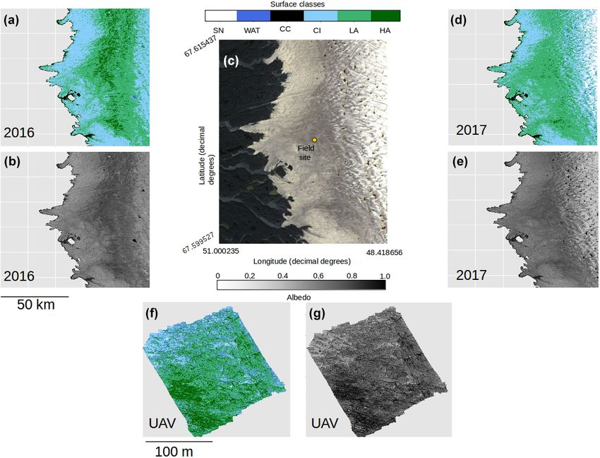
Figure 2. (a) Mass absorption coefficients of the major algal pigments including the purpurogallin-type phenol. (b) Measured spectral albedos
for each surface type (Hbio is heavy biomass loading, Lbio is light biomass loading, CI is clean ice and SN is snow). (c) Plot showing the
natural logarithm of cell abundance against broadband albedo. (d) Microscope image showing examples of both algal species and mineral
fragments from a melted Hbio sample.
Table 1. Composition of each mineral dust “scenario” in percent of total by volume.
Fraction of total (% by volume)
Scenario Quartz Andesite Olivine Enstatite Kaolinite Illite Muscovite
HI-DUST 3.42 67.12 10.53 8.42 3.36 1.70 5.46
LO-DUST 45.39 50.67 3.31 0.64 0 0 0
MN-DUST 24.19 61.03 6.95 3.90 1.37 0.19 2.37
sured 394 ± 194 µgLAP mLice −1 , of which ∼ 95 % was inor- using a constant cell density (0.87 g cm−3 ; Hu, 2014) and
ganic, giving mean and maximum mineral dust loadings of multiplying by our mean and maximum Hbio cell abundance.
373 and 567 µgLAP mLice −1 . Assuming 1 mL of ice to weigh This gave mean and maximum mass mixing ratios of 349
0.917 g, this gives mean and maximum mass mixing ratios and 646 µgalgae gice −1 . We also varied the mass mixing ratios
of 342 and 519 µgdust gice −1 . For glacier algae we calculated over a range of hypothetical values to study the sensitivity
mass mixing ratios by taking the mean cell volume across all of ice surface albedo to dust and glacier algae. Glacier algae
cells in our microscope images, converting to per-cell mass and each of the mineral dusts (LO-DUST, HI-DUST, MN-
The Cryosphere, 14, 309–330, 2020 www.the-cryosphere.net/14/309/2020/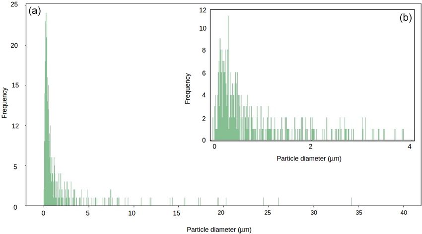
J. M. Cook et al.: Glacier algae accelerate melt rates                                                                         315

DUST) were added individually to the upper 0.1 cm layer in         tent heat of fusion for melting ice (334 J g−1 ) and integrated
mixing ratios of 10, 100, 500 and 1000 µgLAP gice −1 , plus the    over the entire day as described above. This provided a value
mean and maximum measured mass mixing ratios for dust              for the amount of melting caused by the presence of algae
and algae, to quantify their effects on the surface albedo. We     per day assuming the cold content of the ice to be depleted.
also ran a sensitivity study where we repeated the simulations     We calculated uncertainty by running these calculations for
with two other dust types, sourced from previous literature,       every possible combination of our measured algal and clean
with contrasting mineralogies to our field site.                   ice spectra and calculating the mean, standard error, and stan-
                                                                   dard deviation of the pooled results.
2.6   Empirical measurement of mineral dust reflectance               We corroborated these estimates using a point surface en-
                                                                   ergy balance model (Brock and Arnold, 2000; Tedstone,
For two samples of local mineral dusts obtained from Hbio          2019). This model predicts melting in millimetres of wa-
sites, we chemically removed the organic matter and mea-           ter equivalent given local meteorological data and informa-
sured the PSD using scanning electron microscopy (full de-         tion about the ice surface albedo and roughness. We ran this
tails in Sect. S3). The chemical cleaning method avoided the       model with the albedo set equal to the broadband albedo for
artificial “reddening” of the mineral dust sample associated       each clean ice (CI), heavy biomass (Hbio ) and light biomass
with removing organic matter by ignition. We then arranged         (Lbio ) spectrum in our field measurements. The hourly mete-
the mineral dust samples into an optically thick layer on a        orological data for 21 July 2017 used to force the model were
microscope slide and pressed them tightly against the open         from a Delta-T GP1 automatic weather station positioned at
aperture of a Thorlabs IS200-4 integrating sphere to mea-          our field site. The difference in predicted melt between the
sure their reflectance. The other apertures were covered with      algal surfaces and the clean ice surfaces provided the melt
SM05CP2C caps and the sample reflectance was measured              attributed to the presence of algae. As for the radiative forc-
using the same ASD Field Spec Pro 3 as was used for field          ing calculations, the uncertainty was calculated by running
measurements.                                                      the energy balance model for every possible combination of
                                                                   algal and clean ice spectra and calculating the mean, standard
2.7   Radiative forcing and biological melt acceleration           error, and standard deviation of the pooled results.

The biological radiative forcing was calculated by first differ-   2.8   UAV and Sentinel-2 remote sensing
encing the albedo for algal surfaces and the albedo for clean
ice surfaces measured at our field site. This gives the differ-    Having quantified algal melt acceleration in localized
ence in albedo between the clean and algal ice surfaces, αdiff .   patches using the methods described in Sect. 2.2–2.6, we
The product of each αdiff and the incoming irradiance, I ∗ ,       then used a multispectral camera mounted to a UAV to quan-
provided the instantaneous power density (PDalg ) absorbed         tify algal coverage across a 200 × 200 m area at our field site.
by the algae. We assume that photosynthetic processes uti-         This sample area was kept pristine throughout the study pe-
lize 5 % of this absorbed energy – at the upper end of a re-       riod to minimize artefacts of our presence appearing in the
alistic range for photosynthetic microalgae (Blankenship et        UAV imagery. Inside the sampling area we placed fifteen
al., 2011; Masojídek et al., 2013). The remainder of PDalg         10 × 10 cm ground control points (GCPs), whose precise lo-
is conducted into the surrounding ice, giving the instanta-        cation was measured using a Trimble differential GPS. At
neous radiative forcing due to algae (IRFalg ). Since these        these markers we also made ground spectral measurements
cells are coloured by the purple purpurogallin pigment, we         using an ASD-Field Spec Pro 3 immediately after each flight.
assume the reflective radiative forcing to be negligible, as       The UAV itself was a Steadidrone Mavrik-M quadcopter,
demonstrated by Dial et al. (2018). IRFalg was calculated          onto which we integrated a MicaSense Red-Edge multispec-
at hourly intervals using incoming irradiance simulated for        tral camera. The camera is sensitive in five discrete bands,
our field site using the PVSystems solar irradiance program        with centre wavelengths of 475, 560, 668, 717, and 840 nm
(https://pvlighthouse.com.au, last access: July 2019) at 1 nm      and bandwidths of 20, 20, 10, 10, and 40 nm, respectively.
spectral resolution, following Dial et al. (2018). The radiative   The horizontal field of view was 47.2◦ and the focal length
forcing was assumed to be constant between each 1 h time           5.4 mm. The camera was remotely triggered through the au-
step, meaning the radiative forcing over 1 h (HRFalg ) could       topilot, which was programmed along with the flight coordi-
be calculated by multiplying IRFalg by 3600 s h−1 , assuming       nates in the open-source software Mission Planner (Osborne,
that instantaneous radiative forcing is equal to radiative forc-   2019). Images were acquired at approximately 2 cm ground
ing per second. Daily radiative forcing due to algae (RFalg )      resolution with 60 % overlap and 40 % sidelap. The flights
was then calculated as the sum of HRFalg between 00:00 and         were less than 20 min long and at an altitude of 30 m above
23:00 UTC.                                                         the ice surface.
   To calculate the algal contribution to melting (Malg ),            We applied radiometric calibration and geometric dis-
IRFalg was multiplied by 104 to convert the radiative forcing      tortion correction procedures to acquired imagery follow-
from units of W m−2 to W cm−2 and then divided by the la-          ing MicaSense procedures (Micasense, 2019). We then con-

www.the-cryosphere.net/14/309/2020/                                                        The Cryosphere, 14, 309–330, 2020
316 J. M. Cook et al.: Glacier algae accelerate melt rates
verted from radiance to reflectance using time-dependent re- the SVM, the parameters C and gamma were tuned using
gression between images of the MicaSense Calibrated Re- grid search cross validation. Two ensemble classifiers were
flectance Panel acquired before and after each flight (i.e. also trained: a voting classifier that combined the predictions
a regression line was computed between the reflectance of of each of the three individual classifiers and a RF algorithm.
the white reference panel at the start and end of the flight The performance of each classifier was measured using pre-
and used to quantify the change in irradiance during the cision, accuracy, recall, and F1 score and also by plotting the
flight). Finally, the individual reflectance-corrected images confusion matrix and normalized confusion matrix for each
were mosaicked using AgiSoft PhotoScan following pro- classifier. In all cases the RF outperformed the other classi-
cedures developed by the United States Geological Survey fiers according to all available metrics (Sect. S5). The perfor-
(USGS, 2017), yielding a multi-spectral ortho-mosaic with mance of the RF classifier was finally measured on the test
5 cm ground resolution, georectified to our GCPs. There was set, demonstrating the algorithm’s ability to generalize to un-
generally close agreement between the ground, UAV and seen data outside of the training set. Overfitting is not usually
satellite-derived albedo, although there are some differences associated with the RF classifier, and the strong performance
that we believe to be the result of different radiometric cal- on both our training and test sets confirms that the model gen-
ibration techniques for satellite, UAV and ground measure- eralizes well. For these reasons, we used the RF algorithm to
ments, and the differing degrees of spatial integration have classify our multispectral UAV and Sentinel-2 images. Train-
been examined in detail in Tedstone et al. (2019). ing the classifier using data from field spectroscopy ensures
To upscale further, we used multispectral data from the quality of each labelled data point in the training set, since
the Copernicus Sentinel-2 satellite. We selected the our sampling areas were homogeneous and surface samples
100 × 100 km tile covering our field site (T22WEV) on the were analysed in the laboratory, circumventing issues of spa-
closest cloud-free day to our UAV flight on 21 July. The tial heterogeneity and uncertainty in labelling that could lead
L1C product was downloaded from SentinelHub (Sinergise, to ambiguity for direct labelling of aerial images. Compar-
Slovenia). The L1C product was processed to L2A using the isons between the directional reflectance spectra gathered us-
European Space Agency (ESA) Sen2Cor processor, includ- ing the ASD field spectrometer and those measured using the
ing atmospheric correction and reprojection to 20 m resolu- UAV and Sentinel-2 are provided in Fig. 3. Simultaneously
tion. with the surface classification, we calculated the albedo in
each UAV pixel using the narrowband to broadband conver-
2.9 Supervised classification algorithms and albedo sion of Knap et al. (1999) applied to the reflectance at each
mapping of the five bands.
This protocol was repeated for Sentinel-2 imagery. Addi-
To map and quantify spatial coverage of algae over the tional bands are available for use as feature vectors in the
ice sheet surface we employed a supervised classification case of Sentinel-2. Directional reflectance data gathered us-
scheme. A random forest (RF) classifier was trained on the ing the ASD field spectrometer were reduced to only those
field spectra collected on the ice surface (see Sect. 2.3) and nine wavelengths coincident with the centre wavelengths
then applied to multispectral images gathered by the UAV measured by Sentinel-2 at 20 m ground resolution (0.480,
and Sentinel-2. We also included spectra obtained at the same 0.560, 0.665, 0.705, 0.740, 0.788, 0.865, 1.610, 2.190 µm).
field site in July 2016 to our training set, giving a total of 231 Training on reduced hyperspectral data has several advan-
labelled spectra. A schematic of the classification workflow tages over training directly on aerial multispectral data. First,
is provided in Sect. S4. Our HCRF measurements were first the method is sensor agnostic because the classifier can be
reduced to reflectance values at five key wavelengths coinci- retrained with a different selection of wavelengths for other
dent with the centre wavelengths measured by the MicaSense upscaling platforms, enhancing the reusability of the field
Red-Edge camera mounted to the UAV (blue: 0.475; green: measurements. Second, we have confidence in our labels be-
0.560; red: 0.668; red edge: 0.717; NIR: 0.840 µm), yield- cause each sample has been analysed in a laboratory to con-
ing reflectance at each wavelength as a feature vector for firm its composition, reducing label ambiguity. Finally, the
the classifier (in this case the spectral response function of limited field of view of the field spectrometer reduces errors
the camera was not accounted for). The classification labels arising from mixing of spectra from heterogeneous ice sur-
were the surface type as determined by visual inspection: SN faces. Sentinel-2 imagery was masked using the MeASUREs
(snow), CI (clean ice), CC (cryoconite), WAT (water), Lbio Greenland Ice Mapping Project ice mask (Howat, 2017) to
(low-biomass algae) and Hbio (high-biomass algae). For the eliminate non-ice areas. Pixels with more than 30 % prob-
algal surface classes our visual assessment was corroborated ability of being obscured by cloud were masked using the
by microscopy, as described in Sect. 2.2. This dataset was Sentinel-2 L2A cloud product generated by the Sen2Cor pro-
then shuffled and split into a training set (80 %) and a test cessor. For the calculation of albedo in each pixel, the addi-
set (20 %). The training set was used to train three individual tional bands available in the Sentinel-2 images enabled the
supervised classification algorithms: Naive Bayes, k-nearest application of Liang et al.’s (2001) narrowband to broadband
neighbours (KNN) and support vector machine (SVM). For conversion.
The Cryosphere, 14, 309–330, 2020 www.the-cryosphere.net/14/309/2020/J. M. Cook et al.: Glacier algae accelerate melt rates 317
Figure 3. Inter-sensor comparisons. (a–e) Each UAV band reflectance plotted against ASD reflectance in uncorrected (blue) and corrected
(red) form. The correction was applied to account for a systematic offset shown in the header for each plot. (f) Mean reflectance and ±1
standard deviation error bars at each spectral band for each surface class for the ASD field spectrometer and the UAV-mounted multispectral
camera. (g) Mean reflectance and ±1 standard deviation error bars at each spectral band for each surface class for the ASD field spectrometer
and Sentinel-2.
2.10 Comparing 2016 and 2017 whereas the dark zone was especially dark, widespread and
prolonged in 2016 (Fig. 4; Tedstone et al., 2017). We there-
In 2017, the GrIS dark zone had a relatively small spatial fore conducted a comparison between the algal coverage on
extent, high albedo and short duration in comparison to the the same dates in 2016 and 2017. First, we examined varia-
other years in the MODIS record, particularly since 2007, tions in the extent and duration of the dark zone, along with
www.the-cryosphere.net/14/309/2020/ The Cryosphere, 14, 309–330, 2020318 J. M. Cook et al.: Glacier algae accelerate melt rates
snow depths and snow clearing dates for the south-western
ablation zone using MODIS, extending the time series of
Tedstone et al. (2017). Bare ice was mapped by applying a
threshold reflectance value (R < 0.60 at 0.841–0.871 µm) to
the MOD09GA Daily Land Surface Reflectance Collection
6 product. Within the bare-ice area, dark ice was mapped us-
ing a lower reflectance threshold (R < 0.45 at 0.62–0.67 µm).
The area of interest was the “common area” defined by Ted-
stone et al. (2017) bounded within the latitudinal range 65–
70◦ N and is equal to that used by Wang et al. (2018). To
measure the annual dark-ice extent (in km2 ) we counted the
pixels that were dark for at least 5 d each year. The an-
nual duration was defined at each pixel as the percentage
of daily cloud-free observations made in each JJA (June–
July–August) period that were classified as dark. The timing
of bare ice appearance was calculated from MODIS using
a rolling window approach on each pixel (see Tedstone et
al., 2017). The mean snow depths were extracted from out-
puts from the regional climate model MAR v3.8 (Fettweis et
al., 2017) run at 7.5 km resolution forced by ECMWF ERA-
Interim reanalysis data (Dee et al., 2011). These data enabled
a comparison of the extent and timing of dark ice in 2016 and
2017.
To examine algal coverage in each year we identified the
Sentinel-2 tile covering our field site (22WEV) on the closest
cloud-free date to the UAV flight day (21 July) in each year.
These were 26 July 2017 and 25 July 2016. Since we were in-
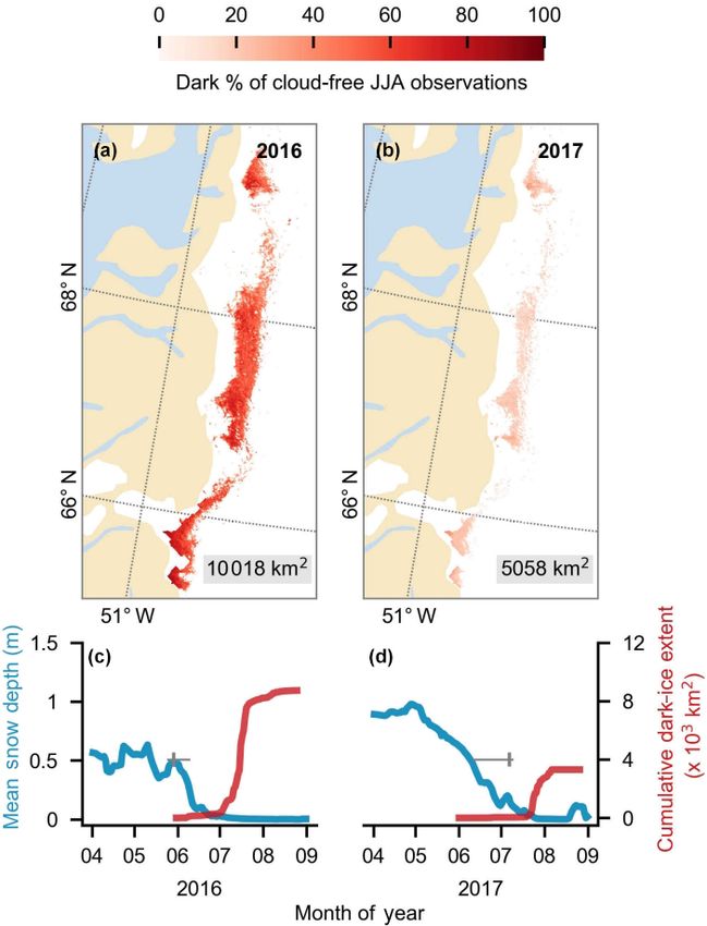
terested in the bare-ice zone, snow-covered pixels were omit- Figure 4. (a, b) Dark-ice duration on the south-western GrIS in
ted from the calculations. summers 2016 and 2017, expressed as a percentage of the total daily
cloud-free observations made during June–July–August (JJA). Each
year is labelled with dark-ice extent. In each year, pixels that are
2.11 Runoff modelling dark for fewer than 5 d are not shown. (c, d) Average snow depth
modelled by MAR (blue) and cumulative dark-ice extent observed
Runoff at the regional scale was calculated using van As by MODIS (red) (Tedstone et al., 2017) during April to August.
et al.’s (2017) surface mass balance (SMB) model, forced Vertical bars (grey) denote median date of snow clearing derived
with local automatic weather station and MODIS albedo ob- from MODIS. Horizontal bars denote the interquartile range of the
servations (van As et al., 2012, 2017). The model interpo- day of year of bare ice appearance. Tick marks denote the start of
lates meteorological and radiative measurements from three each month.
PROMICE automatic weather stations on the K-transect
(KAN-L, KAN-M and KAN-U) and bins them into 100 m
bare ice was calculated by summing runoff in elevation bins
elevation bands (0 to 2000 m a.s.l.). Surface albedo is from
that had mean daily albedo of less than 0.60. Total summer
MODIS Terra MOD10A1 albedo and is averaged into the
runoff from dark ice only was calculated in the same way
same 100 m elevation bins. For every 1 h time step, the model
but using a 0.39 threshold. The study by van As et al. (2017)
iteratively solves the surface energy balance for the surface
compared the performance of the model with independent
temperature. If energy components cannot be balanced due
observations and found errors to be negligible in the bare-ice
to the 0 ◦ C surface temperature limit, a surplus energy sink
zone.
for melting of snow or ice is included. If surface temperature
To determine the algal contribution to runoff, we used
is greater than the melting point, the surplus energy is used
Eq. (1):
for melting of snow or ice. When calculating turbulent heat
fluxes, aerodynamic surface roughness for momentum was Ralg = Rtot × ((MHbio × CHbio ) + (MLbio × CLbio )), (1)
set to 0.02 and 1 mm for snow and ice, respectively (after van
As et al., 2005, 2012; Smeets and Van den Broeke, 2008). We where Ralg is the runoff due to algae, Rtot is the total runoff
extrapolate modelled runoff across the south-western GrIS from the bare-ice zone calculated using our runoff model,
(65–70◦ N) by deriving the areas of each elevation bin using MHbio and MLbio are the mean percentage of total melt at-
the Greenland Ice Mapping Project (GIMP) digital elevation tributed to algae in Hbio and Lbio areas as calculated by our
model (DEM; Howat et al., 2014). Total summer runoff from energy balance modelling described in Sect. 2.6, and CHbio
The Cryosphere, 14, 309–330, 2020 www.the-cryosphere.net/14/309/2020/J. M. Cook et al.: Glacier algae accelerate melt rates 319
and CLbio are the proportion of Ctot comprised of Hbio and served between broadband albedo and biovolume (calculated
Lbio areas in our UAV or Sentinel-2 images. As discussed as the sum of the products of the mean measured cell volumes
later, the Sentinel-2 algal coverage estimate is conservative and the cell counts for each algal species), but the coefficient
because it often fails to resolve Hbio surfaces and therefore of determination was lower (r 2 = 0.42). This may well be the
provides a lower bound on the runoff attributed to algae. result of larger cells having a smaller effect on albedo than
An upper bound was therefore also calculated by assuming more numerous, smaller cells for a given total volume. The
the spatial coverage derived from our UAV remote sensing relationship between absorption and scattering coefficients
– which can accurately distinguish Lbio and Hbio – surfaces and cell size may also not be straightforward for algal cells
is representative of the south-western dark zone. We were due to an increasingly important contribution to the cell op-
thereby able to estimate upper and lower limits for the runoff tical properties from internal heterogeneity, organelles, cell
attributed to algal growth on the south-western ablation zone. walls and the pigment packaging effect in larger cells (Morel
and Bricaud, 1981; Haardt and Maske, 1987).
The albedo of Hbio and Lbio surfaces is depressed in the
3 Results and discussion visible wavelengths (0.40–0.70 µm, Fig. 2b), creating a red-
edge spectrum commonly used in other environments as a
3.1 Algae reduce ice albedo marker for photosynthetic pigments (Seager et al., 2005) and
for mapping algae over the GrIS by Wang et al. (2018).
The ice surfaces we studied were divided into four classes de- Chlorophyll a has a specific absorption feature at 0.68 µm
pending upon the algal abundance measured in the melted ice which is hard to discern in the raw spectra but clear in the
samples: high algal abundance (Hbio ), low algal abundance derivative spectra (Fig. 5a) for Hbio and Lbio but not CI and
(Lbio ), clean ice (CI) and snow (SN). The algal abundance SN. This feature has previously been described as “uniquely
(cells mL−1 ) in each class was as follows: Hbio = 2.9×10⁴ ± biological” (Painter et al., 2001) and supports the hypoth-
2.01 × 10⁴ ; Lbio = 4.73 × 10³ ± 2.57 × 10³ ; CI = 625 ± 381; esis that the albedo reduction observed in these samples is
and SN = 0 ± 0 (1 SD). These cell abundances were signifi- primarily due to algae. Our measurements therefore strongly
cantly different between the classes (one-way ANOVA: F = indicate a biological role in reducing the albedo of the GrIS
10.21; p = 3 × 10⁻⁵ ), which Bonferroni-corrected t tests in- surface; however, to test that the lower broadband and spec-
dicated to be due to variance between all four groups. The tral albedo observed on algal surfaces is primarily due to the
dominant species of algae were Mesotaenium berggrenii presence of algal cells, it was also necessary to compare the
and Ancylonema nordenskioldii (Fig. 2d), confirming ob- albedo-reducing effects of the algae to that of local mineral
servations made by Stibal et al. (2017) and Williamson et dust.
al. (2018) in the same region. Their long, thin and approxi-
mately cylindrical morphology has been shown to be near- 3.2 Algae have greater impact on albedo than mineral
optimal for light absorption (Kirk, 1976). The albedo of dust
the ice surface also varied significantly between the sur-
face classes (one-way ANOVA for broadband albedo: F = Radiative-transfer simulations demonstrated that at measured
7.9; p = 2.8 × 10⁻⁴ ), again with Bonferroni-corrected t tests mass mixing ratios mineral dusts only have a very small
showing variance between all four groups (Sect. S6a, b). (< 0.003) albedo-reducing effect at our field site on the
Greater algal abundance was associated with lower albedo, south-western GrIS, whereas glacier algae reduce the ice
with the albedo reduction concentrated in the visible wave- albedo by up to 0.06, not accounting for indirect albedo-
lengths (Fig. 2b) where both solar energy receipt and al- reducing feedbacks. The effect of adding the mean measured
gal absorption peak (Cook et al., 2017b; Williamson et mass mixing ratio of MN-DUST to the clean ice was a very
al., 2018), diminishing towards longer near infra-red (NIR: small albedo reduction of 0.002 (Table 2; Fig. 5b). In con-
> 0.70 µm) wavelengths where ice absorption, represented trast, adding the mean measured mass mixing ratio of glacier
by the effective grain size, is most likely to cause albedo dif- algae reduced the albedo by 0.03, preferentially in the short
ferences (Warren, 1982). A strong inverse correlation (Pear- visible wavelengths in a similar way to our field-measured
son’s R = 0.75, p = 2.74 × 10⁻⁹ ) was observed between the reflectance spectra (Table 2; Fig. 5b). This effect was greater
natural logarithm of algal cell abundance (cells mL−1 ) in the when the mass mixing ratio was increased to the maximum
surface ice samples and broadband albedo (Fig. 2c). The measured values (646 µgalgae gice −1 and 519 µgdust gice −1 )
linear regression coefficient of determination between the which caused an albedo reduction of 0.06 for glacier algae
albedo and the natural logarithm of cell abundance was 0.57. and 0.003 for MN-DUST. Changing the proportions of the
It is unsurprising that the cell abundance does not account for minerals in our simulated local dusts had a very small effect
all variation in albedo because there are also albedo-reducing on the albedo reduction. At the mean measured mass mix-
effects related to the physical structure of the ice and pres- ing ratio, HI-DUST reduced the albedo by just 0.0023, while
ence of melt water (as demonstrated for snow by, for ex- LO-DUST reduced the albedo by 0.0016. Even with a mass
ample, Warren, 1982). An inverse relationship was also ob- mixing ratio of 1000 µgdust gice −1 , the albedo reduction due
www.the-cryosphere.net/14/309/2020/ The Cryosphere, 14, 309–330, 2020320 J. M. Cook et al.: Glacier algae accelerate melt rates
Figure 5. (a) The first and second derivative spectra for each surface class. (b) BioSNICAR-GO modelled spectral albedo for clean ice (blue)
and ice with each of the simulated local dusts and algae in their measured mass mixing ratios in the upper 1 mm. (c) Reflectance for an
optically thick layer of two samples of the local mineral dust.
Table 2. Albedo change relative to clean ice caused by the addition of each LAP to the upper 1 mm of ice in a range of mass mixing ratios
from 10 to 1000 µgLAP gice −1 .
Hypothetical mass mixing ratios (µgLAP gice −1 ) Measured mass mixing ratios (µgLAP gice −1 )
10 100 500 800 1000 342 349 519 646
Glacier algae −0.0010 −0.0110 −0.0460 −0.0670 −0.0800 −0.030 −0.040 −0.0487 −0.056
HI-DUST −0.0001 −0.0006 −0.0030 −0.0048 −0.0060 −0.0021 −0.0023 −0.0033 −0.0039
LO-DUST −0.0001 −0.0004 −0.0021 −0.0034 −0.0042 −0.0015 −0.0016 −0.0023 −0.0028
MN-DUST < 0.0001 < 0.0001 −0.0020 −0.0043 −0.005 −0.001 −0.002 −0.0029 −0.0035
to local mineral dusts was only 0.006, 0.004 and 0.005 for mineral dusts cannot account for the broadband albedo re-
the HI-DUST, LO-DUST and MN-DUST, compared to 0.08 duction observed in the field. This is consistent with the lo-
for glacier algae. cal mineralogy being dominated by weakly absorbing min-
Across all our simulations, the broadband albedo-reducing erals with small grain sizes, as measured in our field sample
power of glacier algae exceeded that of the local min- (Figs. 5c, 6; Table 2). In Sect. S7 we demonstrate that these
eral dusts, often by several orders of magnitude. At field- conclusions are robust to different dust types, including those
measured mass mixing ratios for heavily laden Hbio surfaces, with typically Saharan optical properties and dusts with vary-
The Cryosphere, 14, 309–330, 2020 www.the-cryosphere.net/14/309/2020/J. M. Cook et al.: Glacier algae accelerate melt rates 321 Figure 6. Particle size diameter for our local mineral dust sample (panel (b) shows magnification of 0–4 µm range). ing hematite concentrations. The radiative-transfer simula- tian Land (80◦ N, 24◦ W), but this area is geologically and tions do not account for feedbacks related to grain size and climatologically distinct from our field site and their tran- shape, near-surface meltwater accumulation, and the pres- sect only spanned ∼ 8 km from the ice sheet margin, being ence of other light absorbing particles, such as humic sub- an area prone to local dust deposition. Overall, our study is stances, that might modify the spectral reflectance and ex- consistent with previous studies that have identified that the acerbate the biological albedo reduction. Furthermore, the local bare-ice mineral dust is poor in hematite and rich in albedo-lowering effects of both the glacier algae and min- weakly absorbing quartz and feldspar minerals (e.g. Tedesco eral dusts is reduced by the low albedo of the underlying ice. et al., 2013). Tedesco et al. (2013) reported their dusts be- In simulations using smaller diameter, higher-albedo snow ing redder than algae. However, their minerals were sourced grains (whose optical properties were estimated using Mie from cryoconite, not the ice surface, where glacier algae are theory) the albedo reduction caused by 1000 µgdust gice of scarce and the biota is dominated by a rich consortium of MN-DUST increased to 0.009, 0.010 and 0.012 for grains other microbes that lack the characteristic pigmentation of of diameter 1500, 1000 and 500 µm, respectively. glacier algae. Furthermore, Tedesco et al. (2013) reported an The small direct albedo-reducing effect from local miner- average of only 0.3 % goethite in their Greenland cryoconite als on the ice surface is seemingly in contrast to some pre- samples. This may have been present as hematite prior to vious studies, such as Wientjes et al. (2010, 2011) and Bøg- their sample processing, which involved heating the samples gild (2010); however, we highlight that neither of the Wien- to 500–1000 ◦ C. This heating treatment likely oxidized Fe- tjes et al. (2010, 2011) studies directly measured the surface bearing mineral phases, thereby artificially introducing the albedo or any optical properties of the mineral dusts retrieved observed reddening. from their GrIS sampling sites and only inferred mineralogi- While these radiative-transfer simulations indicate that cal darkening from low spectral resolution MODIS data and mineral dust is unlikely to be directly causing the albedo the presence of a “wavy pattern” observed across the dark decline on the GrIS, they may still influence the ice albedo zone. We argue that while this may be indicative of geolog- indirectly by acting as substrates for the formation of low- ical outcropping onto the ablation zone, it does not neces- albedo microbial mineral aggregates known as cryoconite sarily follow that these minerals are responsible for surface granules, which are often found in quasi-cylindrical melt darkening. In support of this, Wientjes et al. (2011) found holes or scattered over ice surfaces (Wharton et al., 1985; strongly scattering and weakly absorbing quartz to be the Cook et al., 2015a) or by providing a nutrient source stim- dominant mineral in surface ice and speculated that biota ulating algal growth (Stibal et al., 2017). This is especially may be having a darkening effect. Bøggild et al. (2010) found true because there is evidence in the previous literature that mineral dust to be an albedo reducer in Crown Prince Chris- the dust present on the GrIS bare-ice surface is likely derived www.the-cryosphere.net/14/309/2020/ The Cryosphere, 14, 309–330, 2020
You can also read