Implications of model selection: a comparison of publicly available, conterminous US-extent hydrologic component estimates - HESS
←
→
Page content transcription
If your browser does not render page correctly, please read the page content below
Hydrol. Earth Syst. Sci., 25, 1529–1568, 2021
https://doi.org/10.5194/hess-25-1529-2021
© Author(s) 2021. This work is distributed under
the Creative Commons Attribution 4.0 License.

Implications of model selection: a comparison of publicly available,
conterminous US-extent hydrologic component estimates
Samuel Saxe1,2 , William Farmer1 , Jessica Driscoll1 , and Terri S. Hogue2,3
1 Analysisand Prediction Branch, U.S. Geological Survey, Lakewood, CO 80225, USA
2 HydrologicScience and Engineering, Colorado School of Mines, Golden, CO 80401, USA
3 Department of Civil and Environmental Engineering, Colorado School of Mines, Golden, CO 80401, USA

Correspondence: Samuel Saxe (ssaxe@usgs.gov)

Received: 8 May 2020 – Discussion started: 5 June 2020
Revised: 16 December 2020 – Accepted: 11 January 2021 – Published: 26 March 2021

Abstract. Spatiotemporally continuous estimates of the hy-     the greatest emphasis on storage and runoff components, to
drologic cycle are often generated through hydrologic mod-     better describe complexities of the terrestrial hydrologic sys-
eling, reanalysis, or remote sensing (RS) methods and are      tem and reconcile model disagreement.
commonly applied as a supplement to, or a substitute for,
in situ measurements when observational data are sparse or
unavailable. This study compares estimates of precipitation
(P ), actual evapotranspiration (ET), runoff (R), snow water   1   Introduction
equivalent (SWE), and soil moisture (SM) from 87 unique
data sets generated by 47 hydrologic models, reanalysis data   A long-term goal of the atmospheric and hydrologic scien-
sets, and remote sensing products across the conterminous      tific communities has been to produce accurate estimates of
United States (CONUS). Uncertainty between hydrologic          the hydrologic cycle across continental and global domains
component estimates was shown to be high in the western        (Archfield et al., 2015; Beven, 2006; Freeze and Harlan,
CONUS, with median uncertainty (measured as the coeffi-        1969). Various methodologies have been applied to meet this
cient of variation) ranging from 11 % to 21 % for P , 14 %     goal, typically in the form of physically based, reanalysis,
to 26 % for ET, 28 % to 82 % for R, 76 % to 84 % for SWE,      or remote-sensing-based models. Many of the resulting esti-
and 36 % to 96 % for SM. Uncertainty between estimates was     mates are made publicly available by an assortment of sci-
lower in the eastern CONUS, with medians ranging from 5 %      entific entities at both continental and global extents across
to 14 % for P, 13 % to 22 % for ET, 28 % to 82 % for R, 53 %   a wide range of spatiotemporal resolutions. These data sets
to 63 % for SWE, and 42 % to 83 % for SM. Interannual          accelerate progress in the atmospheric and hydrologic sci-
trends in estimates from 1982 to 2010 show common dis-         ences by filling knowledge gaps in data-sparse regions, re-
agreement in R, SWE, and SM. Correlating fluxes and stores     ducing the need for time-consuming and computationally ex-
against remote-sensing-derived products show poor overall      pensive modeling, and by providing numerous estimates to
correlation in the western CONUS for ET and SM estimates.      apply within ensemble analyses.
Study results show that disagreement between estimates can         Publicly available modeled estimates have been applied
be substantial, sometimes exceeding the magnitude of the       to work on water budget analyses (Gao et al., 2010; Pan
measurements themselves. The authors conclude that mul-        et al., 2012; Rodell et al., 2015; Smith and Kummerow,
timodel ensembles are not only useful but are in fact a ne-    2013; Velpuri et al., 2019; Zhang et al., 2018), the effects
cessity for accurately representing uncertainty in research    of climate change (La Fontaine et al., 2015; G. J. McCabe
results. Spatial biases of model disagreement values in the    et al., 2017), and water availability and use (Landerer and
western United States show that targeted research efforts in   Swenson, 2012; Thomas and Famiglietti, 2019; Voss et al.,
arid and semiarid water-limited regions are warranted, with    2013; Zaussinger et al., 2019). Rapid increases in compu-
                                                               tational power and data accessibility following the advent of

Published by Copernicus Publications on behalf of the European Geosciences Union.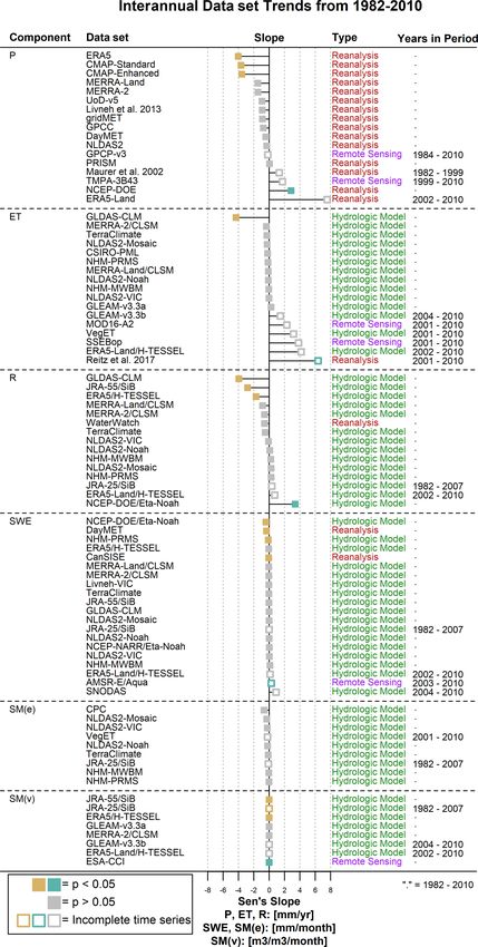
1530                   S. Saxe et al.: A comparison of publicly available, CONUS-extent hydrologic component estimates

early global- and continental-extent hydrologic models in the        a range of ecological regimes. We differentiate this work
1980s and 1990s (Koster and Suarez, 1992; Manabe, 1969;              from previous model intercomparison and validation stud-
Sellers et al., 1986; Yang and Dickinson, 1996), and increas-        ies by placing results in the context of multiple water budget
ingly higher-resolution passive and active satellite measure-        analyses. We seek to quantify how estimates of component
ments of both the surface and subsurface of the Earth (Als-          magnitudes and long-term trends differ in the conterminous
dorf et al., 2007; M. F. McCabe et al., 2017), have led to an        United States (CONUS) and within ecologically distinct re-
explosion in the production of multidecadal, continental- to         gions. The primary goal of this work is to quantify model
global-extent models estimating all major components of the          disagreement in terms of magnitude, interannual trend, and
hydrologic cycle (Peters-Lidard et al., 2018). Accordingly,          correlation against remote sensing (RS) products. The effects
this has given rise to a multitude of model comparison and           of model disagreement are shown in regional water budget
evaluation projects throughout the scientific literature.            analyses. We undertake a robust comparison of P , ET, R,
   Earlier model intercomparison projects, such as the Cou-          SWE, and SM estimates generated through hydrologic mod-
pled Model Intercomparison Project (CMIP; Covey et al.,              els, reanalysis data sets, and remote sensing products. We it-
2003), the Integrated Hydrologic Model Intercomparison               eratively calculate water budget imbalances in eight regions
Project (IH-MIP; Kollet et al., 2017; Maxwell et al., 2014),         by applying a range of flux estimates to quantify how model
the Agricultural Model Intercomparison and Improvement               selection may impact residuals.
Project (AgMIP; Rosenzweig et al., 2013), and the Water
Model Intercomparison Project (WaterMIP; Haddeland et al.,
2011), provide robust analyses aimed at attributing differ-          2     Methods and data
ences in model process representation to differences in model
                                                                     2.1     Data categories
design, parameter selection, and meteorological forcings.
   Detailed comparisons between smaller selections of mod-           Hydrologic estimates are divided into water budget flux com-
els are often included in studies presenting novel products          ponents of P , ET, and R, and storage components of SWE
(Daly et al., 2008; Senay et al., 2011; Velpuri et al., 2013;        and SM, representing the primary fluxes and stores of a sur-
Xia et al., 2012a, b). Furthermore, a range of studies have          face water budget. Data sets were selected by prioritizing
focused solely on the validation of third-party models, ei-          public availability, ease of access, and relative use within
ther examining multiple water budget components simulta-             the research community. These data sets are subdivided into
neously (Gao et al., 2010; Sheffield et al., 2009) or focus-         loosely defined categories of hydrologic models, reanalysis
ing on specific components such as precipitation (P ; Derin          data sets, and remote-sensing-derived products. References
and Yilmaz, 2014; Donat et al., 2014; Guirguis and Avissar,          and spatiotemporal information for each data set are provided
2008; Prat and Nelson, 2015; Sun et al., 2018), evapotranspi-        in Table 1, and more detailed long-form descriptions are pro-
ration (ET; Carter et al., 2018; McCabe et al., 2016), snow          vided in Appendix A.
water equivalent (SWE; Broxton et al., 2016; Chen et al.,
2014; Dawson et al., 2016, 2018; Essery et al., 2009; Mudryk         2.1.1    Hydrologic models
et al., 2015; Rutter et al., 2009; Vuyovich et al., 2014), or soil
moisture (SM; Brocca et al., 2011; Koster et al., 2009; Xia et       The hydrologic model category (Table 1; Appendix A) in-
al., 2014).                                                          cludes any estimates generated using equations or concepts
   Most of these comparison studies have revolved around er-         attempting to represent real-world hydrology. Model output
ror metrics derived through validation against in situ and ex        differences are strongly controlled by forcing data sets (El-
situ measurements. However, validation often yields unsat-           sner et al., 2014; Mizukami et al., 2014), calibration meth-
isfactory representations of model skill. Observational data         ods (Mendoza et al., 2015), applied equations (Clark et al.,
sets are often spatiotemporally discontinuous, and model es-         2015a), model structure (Clark et al., 2015a, b), and geophys-
timates in grid structure may not sufficiently represent the         ical parameter availability (Beven, 2002; Bierkens, 2015;
sub-grid heterogeneity that is present in point data, espe-          Mizukami et al., 2017). The most common hydrologic mod-
cially in topographically and ecologically complex regions.          els this study evaluates are conceptual and physically based.
Furthermore, observational measurements can have signifi-            Conceptual models derive terrestrial hydrology estimates
cant associated uncertainty (Di Baldassarre and Montanari,           through empirical relationships between fluxes and stores,
2009). Validation literature is heavily focused on the compar-       typically through a water balance model (WBM) in the style
ison of error statistics and spatial summaries of model skill        of Thornthwaite (1948; NHM-MWBM and TerraClimate).
and rarely discusses the effect of model disagreement on re-         Physically based models utilize meteorological forcing data
search results.                                                      and solve equations describing physical conservation laws
   This research seeks to supplement past comparison and             of mass, energy, and momentum. These can be further sub-
validation literature by evaluating how uncertainty between          divided by targeted hydrologic variables as follows: land sur-
publicly available water budget component estimates used             face models (LSMs) target land–atmosphere interactions, es-
within a study can control outcomes and conclusions across           pecially ET, while catchment models (CMs) target stream-

Hydrol. Earth Syst. Sci., 25, 1529–1568, 2021                                         https://doi.org/10.5194/hess-25-1529-2021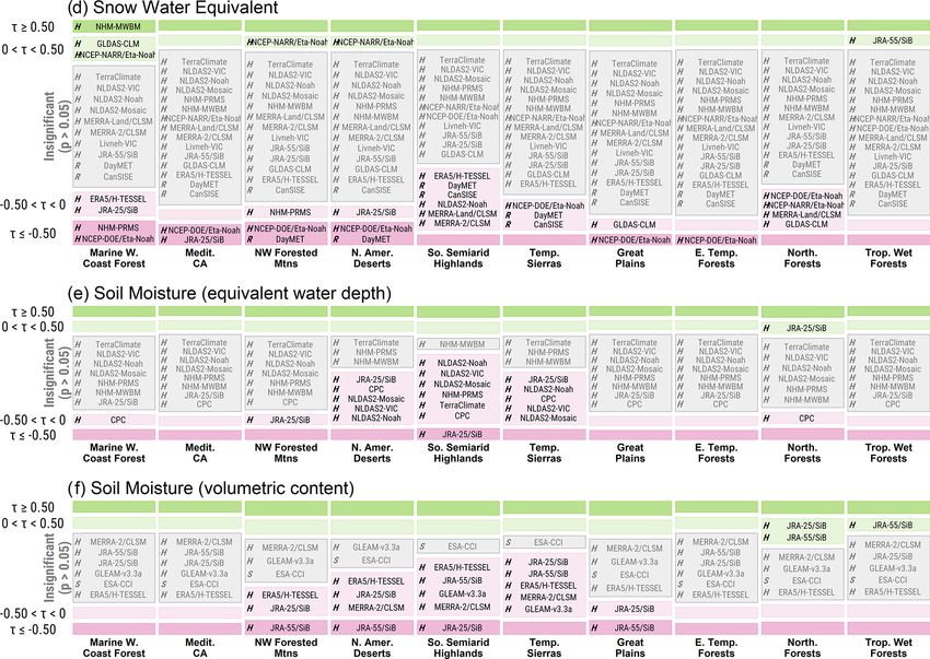
S. Saxe et al.: A comparison of publicly available, CONUS-extent hydrologic component estimates                                     1531

Table 1. Summary of data sets used in this research, including assigned data category, abbreviated name, primary organization, literature
reference, spatiotemporal resolution, and sourced hydrologic components. The reader is referred to Appendix A for definitions of abbrevi-
ated model names, descriptions, and further references. Components are precipitation (P ), evapotranspiration (ET), runoff (R), snow water
equivalent (SWE), and soil moisture in equivalent water depth and volumetric water content (SM(e) and SM(v), respectively). Hydrologic
models NMH-MWBM and NMH-PRMS are based on a delineated (i.e., non-gridded), topographically derived spatial framework composed
on hydrologic response units (HRUs). The reanalysis product WaterWatch is generated at hydrologic units (HUs) 2–8. The finest-resolution
product, HU8, is used in this study.

      Data set                   Group           Reference                              Spatiotemporal         Components
      Hydrologic model
      CPC                        CPC             Fan and van den Dool (2004)        1/2◦      1948–present     SM(e)
      CSIRO-PMLc                 CSIRO           Zhang et al. (2016)                1/2◦      1981–2012        ET
      ERA5/H-TESSELc             ECMWF           Muñoz Sabater (2019)               1/4◦      1979–present     R, SWE, SM(v)
      ERA5-Land/H-TESSEL         ECMFW           Muñoz Sabater (2019)               1/10◦     2001–present     ET, R, SWE, SM(v)
      GLDAS-CLMc                 NASA            Rodell et al. (2007)               1◦        1979–present     ET, R, SWE
      GLEAMa, c                  U. of BE        Martens et al. (2017)              1/4◦      1980–present     ET, SM(v)
      JRA-25/SiB                 JMA             Onogi et al. (2007)                110 km    1979–present     R, SWE, SM(e)/(v)
      JRA-55/SiBc                JMA             Kobayashi et al. (2015)            55 km     1957–present     R, SWE, SM(v)
      Livneh-VIC                 CIRES           Livneh et al. (2013)               1/16◦     1915–2011        SWE
      MERRA-Land/CLSMc           NASA            Reichle et al. (2011)              1/2◦      1980–2016        ET, R, SWE
      MERRA-2/CLSMc              NASA            Reichle et al. (2017)              1/2◦      1980–present     ET, R, SWE, SM(v)
      NCEP–DOE/Eta-Noahc         NOAA            Kanamitsu et al. (2002)            210 km    1979–present     R, SWE
      NCEP-NARR/Eta-Noah         NOAA            Mesinger et al. (2006)             32 km     1979–present     SWE
      NHM-MWBMc                  USGS            McCabe and Markstrom (2007)        HRU       1949–2010        ET, R, SWE, SM(e)
      NHM-PRMSc                  USGS            Regan et al. (2018)                HRU       1980–2016        ET, R, SWE, SM(e)
      NLDAS2-Mosaicc             NASA            Xia et al. (2012a)                 1/8◦      1979–present     ET, R, SWE, SM(e)
      NLDAS2-Noahc               NASA            Xia et al. (2012b)                 1/8◦      1979–present     ET, R, SWE, SM(e)
      NLDAS2-VICc                NASA            Xia (2012c)                        1/8◦      1979–present     ET, R, SWE, SM(e)
      SNODAS                     NWS             Barrett (2003)                     1 km      2003–present     SWE
      TerraClimatec              U. of ID        Abatzoglou et al. (2018)           1/24◦     1958–present     ET, R, SWE, SM(e)
      VegETc                     USGS            Senay (2008)                       1 km      2000–2014        ET, SM(e)
      Reanalysis
      CanSISE                    U. Toronto      Mudryk and Derksen (2017)          1◦        1981–2010        SWE
      CMAPb, c                   CPC             Xie and Arkin (1997)               2 1/2◦    1979–present     P
      Daymetc                    ORNL            Thornton et al. (2018)             1 km      1980–present     P , SWE
      ERA5c                      ECMWF           Muñoz Sabater (2019)               1/4◦      1979–present     P
      ERA5-Land                  ECMWF           Muñoz Sabater (2019)               1/10◦     2001–present     P
      GPCCc                      GPCC            Becker et al. (2013)               1/2◦      1901-2013        P
      gridMETc                   U. of ID        Abatzoglou (2013)                  1/24◦     1979–present     P
      Livneh et al. (2013)c      NOAA            Livneh et al. (2013)               1/16◦     1915–2011        P
      Maurer et al. (2002)       U. WA           Maurer et al. (2002)               1/8◦      1950–1999        P
      MERRA-Landc                NASA            Rienecker et al. (2011)            1/2◦      1980–2016        P
      MERRA-2c                   NASA            Gelaro et al. (2017)               1/2◦      1980–present     P
      NCEP–DOEc                  NCEP–DOE        Kanamitsu et al. (2002)            210 km    1979–present     P
      NLDAS2c                    NASA            Xia et al. (2009)                  1/8◦      1979–present     P
      PRISMc                     OSU             PRISM Climate Group (2004)         4 km      1895–present     P
      Reitz et al. (2017)c       USGS            Reitz et al. (2017)                800 m     2000–2013        ET
      UoD-v5c                    U. of DE        Willmott and Matsuura (2001)       1/2◦      1950–1999        P
      WaterWatchc                USGS            Jian et al. (2008)                 HU8       1901–present     R

https://doi.org/10.5194/hess-25-1529-2021                                            Hydrol. Earth Syst. Sci., 25, 1529–1568, 2021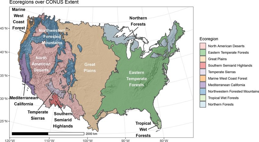
1532                      S. Saxe et al.: A comparison of publicly available, CONUS-extent hydrologic component estimates

Table 1. Continued.

                        Data set                Group           Reference                            Spatiotemporal              Components
                        Remote sensing
                        AMSR-E/Aqua             NSIDC           Tedesco et al. (2004)           25 km       2002–2011            SWE
                        ESA-CCI                 ESA             Dorigo et al. (2017)            1/4◦        1978–present         SM(v)
                        GPCP-v3c                NASA            Huffman et al. (2019)           1/2◦        1983–2016            P
                        MOD16-A2c               U. of MT        Running et al. (2017)           1 km        2000–2010            ET
                        SMOS-L4                 FNCSR           Al Bitar et al. (2013)          25 km       2010–2017            SM(v)
                        SSEBopc                 USGS            Senay et al. (2013)             1 km        2000–2014            ET
                        TMPA-3B43c              NASA            Huffman et al. (2010)           1/4◦        1998–present         P
                      a Versions 3.3a and 3.3b. b Standard and enhanced versions. c Data sets used in the water budget case study with complete data
                      for water years 2001–2010.

flow (Archfield et al., 2015). Additionally, LSMs are often                             models. The reasons for this are two-fold, i.e., (1) to sim-
1D models that operate at discrete spatial intervals, typically                         plify reporting of results and discussion across water bud-
grid cells, lacking horizontal transfer of surface or subsur-                           get components, and (2) although interpolation-based prod-
face water between regions. CMs, on the other hand, uti-                                ucts are often used as reference data sets in model valida-
lize 2D model structures by routing overland and subsur-                                tion studies, especially for precipitation, accuracy decreases
face flows between spatial domains to better realize sur-                               in regions with sparse observations and complex topography
face and groundwater estimates using prescribed stream net-                             (Hofstra et al., 2008) and, thus, should be considered mod-
works. The CLSM, described in the literature as a land sur-                             eled products.
face model (Koster et al., 2000), is discussed in conjunction
with the NHM-PRMS because of the sub-grid catchment net-                                2.1.3      Remote sensing derived
work used to model horizontal runoff and streamflow fluxes.
LSMs are the most common hydrologic model here (e.g.,                                   The RS-derived data sets (Table 1; Appendix A) are compo-
CLM, H-TESSEL, Mosaic, Noah, SiB, and VIC) because                                      nents of the hydrologic system derived from passive and/or
they are often coupled with global-extent atmospheric re-                               active ex situ observations. We note the use of the term RS-
search and, thus, more commonly operated at the spatial ex-                             derived rather than RS because none of the data sets used
tent of this study, while CMs are more typically operated at                            here can be truly described as direct observations as they are
the catchment or basin scale. Additional products included                              always relying on a range of modeling techniques to create
in the hydrologic model category are those using simpli-                                hydrologic estimates. For example, the AMSR-E/Aqua SWE
fied WBMs falling outside the conceptual model paradigm                                 product uses a sequence of steps including a snow-detection
(CPC, CSIRO-PML, GLEAM, and VegET) and those using                                      routine, followed by a physical retrieval algorithm, which is
component-specific physically based models (SNODAS).                                    then validated against observational SWE data (Chang and
                                                                                        Rango, 2000), and the SSEBop product uses a radiation-
2.1.2   Reanalysis                                                                      driven energy balance model to estimate ET (Senay et al.,
                                                                                        2013). Remote sensing data sets include estimates modeled
Reanalysis data sets (Table 1; Appendix A) assimilate multi-                            from single-sensor ex situ observations (MOD16-A2 and
source in situ and ex situ observational data into spatiotempo-                         SSEBop), though most utilize an assembly of information
rally continuous 4D estimates of continental- or global-scale                           from both passive and active sensors at various spatiotempo-
atmospheric and meteorological fluxes using numerical al-                               ral resolutions (e.g., ESA-CCI and GPCP-v3).
gorithms. This category includes reanalysis data sets derived
solely from in situ and ex situ data (e.g., CMAP, Daymet,                               2.2     Data processing
Maurer et al., 2002, and UoD-v5) and those assimilating or
blending multiple reanalysis products with or without obser-                            Data sets included in this research cover a broad spectrum
vational measurements (e.g., CanSISE, gridMET, Livneh et                                of spatial resolutions, extents, coordinate reference systems,
al., 2013, and NLDAS2). In past studies, reanalysis models                              and timescales and, therefore, require a uniform spatiotem-
were often grouped and defined separately from gridded data                             poral system to better facilitate comparison. To that end,
sets derived through statistical interpolation of in situ obser-                        gridded (e.g., NLDAS2-Mosaic) and polygonal (e.g., NHM-
vations (e.g., WaterWatch, Reitz et al., 2017, and GPCC).                               PRMS) data sets were aggregated by area-weighted mean
We combine the two categories, defining the single reanaly-                             to 10 Environmental Protection Agency Ecoregions, Level I
sis category as containing products not generated solely from                           (Omernik and Griffith, 2014), that encompass the Water-
remote sensing observations or through terrestrial hydrologic                           shed Boundary Dataset hydrologic units (U.S. Geological

Hydrol. Earth Syst. Sci., 25, 1529–1568, 2021                                                                  https://doi.org/10.5194/hess-25-1529-2021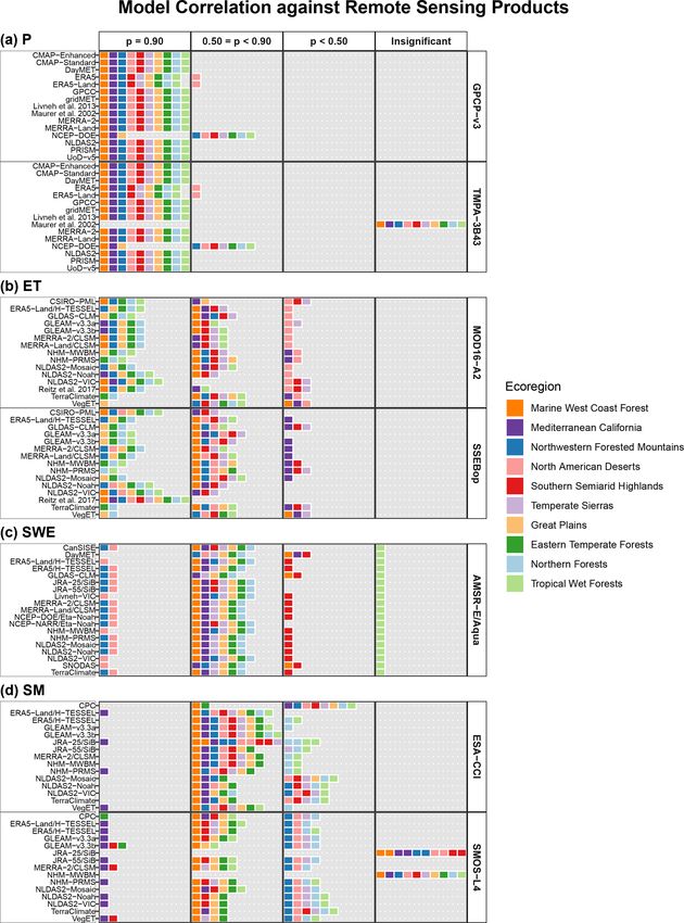
S. Saxe et al.: A comparison of publicly available, CONUS-extent hydrologic component estimates                                           1533

Table 2. Sizes of study ecoregions in square kilometers (km2 ) and              R) were derived by summing monthly values to WYs, and
percent (%) of study domain.                                                    storage terms were derived by averaging monthly values by
                                                                                WY. Incomplete WYs (n months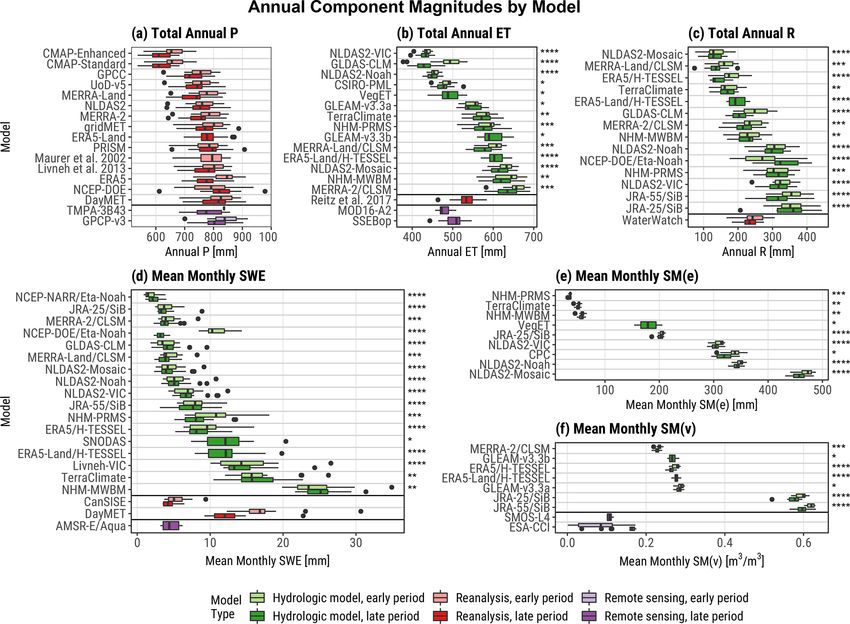
1534                   S. Saxe et al.: A comparison of publicly available, CONUS-extent hydrologic component estimates

Figure 1. Distribution of the 10 ecoregions covering the CONUS study domain.

are converted to a scale of 50 % to 100 % with the following:        increases. With a n : c ranging from 11 : 3 to 16 : 3, maxi-
                                                                     mum possible u in this trend analysis is approximately 0.71.
            p+            p+ > 50

                                                                        Spearman’s rho (Spearman, 1904) is applied to quantify
pD =                               ,                         (3)
            100 % − p +   p + < 50                                   the correlation between RS components P , ET, SWE, and
                                                                     SM and the analogous components of hydrologic models
where pD is the directionalized percent direction colored ac-        and remote sensing data sets. Spearman’s rho (ρ), a non-
cording to the dominant direction value. Positive pD uses a          parametric rank correlation metric, is used to estimate corre-
green gradient, and negative pD uses a purple gradient.              lation, producing values on a −1 to 1 scale, where 1 is perfect
                                                                     positive correlation and −1 is perfect negative correlation, as
2.3.3   Interannual trend                                            follows:
                                                                                 6 di2
                                                                                   P
Both the Mann–Kendall trend test (τ ; Kendall, 1938) and             ρ =1−                 ,                                     (4)
Sen’s slope estimator (Sen, 1968) are used to identify and                      n(n2 − 1)
measure monotonic trends in annual values over WYs 1982–             where d is the difference between ranks, and n is the sam-
2010. Trend significance is evaluated using p values (p) in a        ple size. A binary significance test is used to test correlation
binary significance test, assuming an alpha (α) of 0.05 and a        statistics, assuming α = 0.05, and a null hypothesis that there
null hypothesis of no monotonic trend. Under the condition           is no relationship between data sets. If pα, the null hypothesis is not rejected. Dis-        Correlation is computed and assessed along the monthly time
agreement in the presence of a significant trend and trend di-       step, requiring a minimum of 48 months of temporal overlap
rection is quantified using the unalikeability coefficient (u),      between the modeled estimates and remote sensing data set.
which measures how often categorical variables differ on
a 0 ≤ u ≤ 1 scale, with 0 and 1 being complete agreement             2.3.4     Water budget imbalances
and disagreement, respectively (Kader and Perry, 2007). This
study compares trends between 11 to 16 different products            Water budgets are calculated assuming a steady-state system
(11 ≤ n ≤ 16), depending on water budget component, and              and are solved for imbalances by the following:
uses categorical values (c) of (a) significant negative trend,       P = AET + R + ε,                                             (5)
(b) significant positive trend, and (c) no significant trend, de-
                                                                     ε = P − AET − R,                                             (6)
rived from the direction (sign) and significance (α = 0.05) of
τ . When n>c, maximum possible u decreases from one ex-              where ε is imbalances. Imbalances, ε, cannot be accurately
ponentially to an asymptote of two-thirds as the ratio of n : c      defined as residuals. In reality, ε is the sum of excluded fluxes

Hydrol. Earth Syst. Sci., 25, 1529–1568, 2021                                         https://doi.org/10.5194/hess-25-1529-2021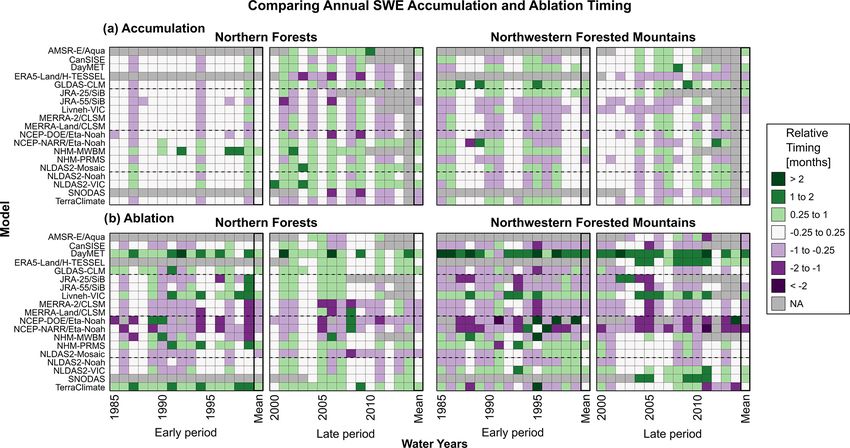
S. Saxe et al.: A comparison of publicly available, CONUS-extent hydrologic component estimates                                  1535

in addition to model uncertainty (residuals). Excluded fluxes
include both natural (e.g., groundwater recharge and changes
to long-term storage) and anthropogenic (e.g., groundwater
extraction) hydrologic processes. Relative imbalances (Rε)
are calculated to better compare water budget results between
regions of varying hydrologic flux by weighting water budget
ε against the total input P as follows:
Rε = (ε/P ) × 100 %.                                       (7)
Water budget relative imbalances were calculated from
summed P , ET, R, and ε over the 10 water year period of
2001–2010 for 15 P , 15 ET, and 13 R estimates (noted in Ta-
ble 1) with temporally continuous monthly data for 10 ecore-
gions. Each ecoregion yielded 2925 water budgets by iter-
ating through all possible combinations of models, totaling
29 250 water budgets in primary regions of the CONUS. In
addition, a single water budget was calculated for each of
the eight ecoregions using the ensemble means of the model        Figure 2. Mean annual (a) standard deviation (σ ) and (b) coefficient
estimates over the same period.                                   of variation (CV) calculated between CONUS-extent modeled esti-
                                                                  mates of hydrologic components precipitation (P ), evapotranspira-
                                                                  tion (ET), runoff (R), snow water equivalent (SWE), soil moisture
3     Results                                                     in equivalent water depth (SM(e)), and soil moisture in volumetric
                                                                  water content (SM(v)). Whiskers on each bar represent the standard
3.1     CONUS domain average                                      deviation of annual values.

3.1.1    Magnitude variability

Uncertainties between annual estimates of states and fluxes       However, soil water profiles can change significantly with
of the hydrologic cycle are substantial when averaged over        depth, so attributing model differences strictly by root zone
the CONUS for each studied component (Fig. 2). The ac-            depth definition is more difficult.
tual magnitude of model estimate differences averaged by             Box plots of modeled estimates by water budget com-
water budget component, measured as σ , is similar for P ,        ponent (Fig. 3) demonstrate the annual ranges of magni-
ET, and R (Fig. 2a) and low (6.6 mm per year) for SWE.            tude generated by various products. Precipitation models
However, comparing uncertainty relative to mean magni-            (Fig. 3a) exhibit low overall variability, with median magni-
tude (Fig. 2b), measured as CV, shows that the vertical,          tudes falling within a distinct 100 mm per year (700–800 mm
atmospheric-controlled fluxes of P and ET demonstrate             per year) range. The exceptions to this are the CMAP reanal-
lower intermodel uncertainty than the horizontal flux of R or     ysis data sets, which have a median 647 mm per year.
storage components SWE and SM. The CV statistic shows                Variability among ET estimates (Fig. 3b) is higher, falling
how, due to the low overall magnitude of SWE, small dif-          within a 200 mm per year (435–650 mm per year) range,
ferences in estimates have a substantial effect on magnitude.     though attributing differences to model type (e.g., LSMs
SM, which is often a large overall storage term in the wa-        vs. CMs) is difficult. Generally, CMs (MERRA-2/CLSM,
ter budget, also shows high CV, indicating that uncertainty in    MERRA-Land/CLSM, and NHM-PRMS) and conceptual
estimates of this component may have the largest impact on        WBMs (NHM-MWBM, GLEAM, and TerraClimate) pro-
hydrologic analyses.                                              duce greater annual rates of ET compared to LSMs
   Unfortunately, high-magnitude differences in SM (Fig. 3e,      (NLDAS2-VIC, GLDAS-CLM, and NLDAS2-Noah). Ex-
f) are likely strongly controlled by model-defined soil layer     ceptions to this are the LSMs NLDAS2-MOSAIC and H-
depth and, thus, limit the utility of disagreement statistics.    TESSEL that are more similar in annual ET flux to CMs and
For example, the TerraClimate and NLDAS2-Noah mod-                WBMs. The RS data sets agree more at the CONUS extent
els apply spatially invariant root zone soil depth across the     with lower-magnitude estimates.
model domains (Abatzoglou et al., 2018; Xia et al., 2012a),          Estimates of R show three distinct clusters of CONUS
whereas the NHM-PRMS assumes a variable depth accord-             magnitudes (Fig. 3c) of 130–190, 220–242, and 310–345 mm
ing to vegetative and geophysical parameters (Regan et al.,       per year. The NLDAS2-Noah and NLDAS2-VIC LSMs,
2018). SM(e) estimates are directly controlled by soil depth,     which produced some of the lowest ET rates, fall within
returning values of equivalent water depth. SM(v) differ-         the higher-magnitude R clusters, as do the JRA-driven SiB
ences are likely to be less influenced by soil depth due to in-   models and NHM-PRMS model. The lowest magnitude
herent measurements of fractional volume rather than depth.       estimates are the NLDAS2-Mosaic and ERA5-driven H-

https://doi.org/10.5194/hess-25-1529-2021                                       Hydrol. Earth Syst. Sci., 25, 1529–1568, 2021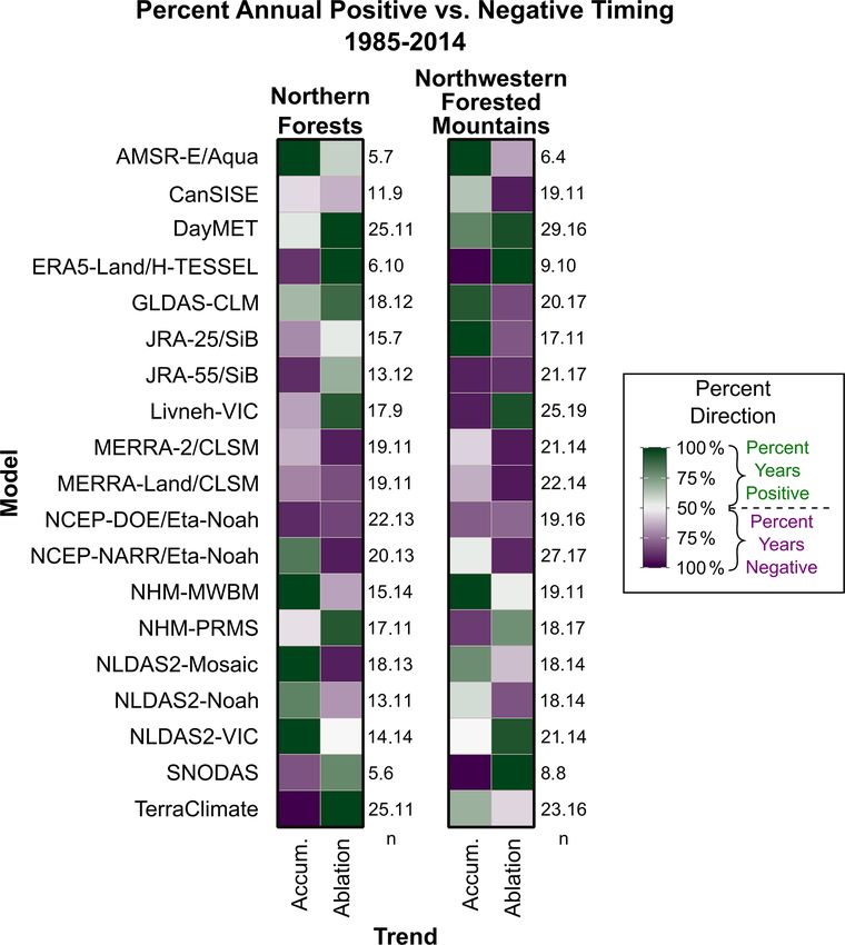
1536                    S. Saxe et al.: A comparison of publicly available, CONUS-extent hydrologic component estimates

Figure 3. Box plots of annual water year magnitudes of all study model estimates averaged over the CONUS extent for hydrologic com-
ponents (a) precipitation (P ), (b) evapotranspiration (ET), (c) runoff (R), (d) snow water equivalent (SWE), (e)soil moisture in units of
equivalent water depth (SM(e)), and (f) soil moisture in units of volumetric water content (SM(v)). Data set magnitudes are subdivided into
two periods, i.e., 1985–1999 (top) and 2000–2014 (bottom), for each model. Flux component estimates (P , ET, and R) are summed from
monthly values to calculate annual water year rates. Storage component estimates (SWE, SM(e), and SM(v)) are averaged from monthly
values to calculate annual water year average storage values. Box lower limits, midlines, and upper limits represent the 25th, 50th (median),
and 75th percentiles, respectively, of the associated data. Whiskers represent 1.5 times the interquartile range. Box color denotes data set
categories of hydrologic model, reanalysis, or remote sensing derived. Asterisks are used to identify the following hydrologic models types:
land surface models (∗∗∗∗ ), catchment models (∗∗∗ ), water balance models (∗∗ ), and miscellaneous (∗ ).

TESSEL LSMs, which are grouped with the CM MERRA-                        or as part of a larger model (e.g., NCEP-NARR/Eta-Noah),
Land/CLSM and WBM TerraClimate. LSMs are more likely                     all estimate lower SWE relative to other data sets. The two
to estimate greater R than WBMs or CMs.                                  VIC LSMs show contrasting median monthly SWE magni-
   Box plots of annually averaged SWE monthly values                     tude over the CONUS, with the Livneh-VIC median exceed-
(Fig. 3d) show that WBMs, notably the NHM-MWBM, gen-                     ing the NLDAS2-VIC median by more than 200 %. The RS
erate much higher SWE than most other data sets. Alterna-                AMSR-E/Aqua product agrees more with lower-magnitude
tively, there are few discernible patterns between the remain-           estimates at the CONUS extent.
ing products, with LSMs and CMs interspersed through-                       Across all water budget components, most data sets
out the gamut of median values. To generalize, the LSMs                  demonstrate lower-magnitude values in the late period (WYs
Noah, GLDAS-CLM, and NLDAS2-Mosaic produce lower-                        2000–2014) compared to the early period (WYs 1985–1999).
magnitude estimates of monthly SWE. A total of three dif-                Within the P flux, almost all data sets agree on a decrease
ferent Noah estimates, driven with different meteorologi-                in the magnitude of hydrologic fluxes from the early to late
cal forcings and run both independently (NLDAS2-Noah)                    periods. This is similarly reflected in the flux estimates of

Hydrol. Earth Syst. Sci., 25, 1529–1568, 2021                                              https://doi.org/10.5194/hess-25-1529-2021
S. Saxe et al.: A comparison of publicly available, CONUS-extent hydrologic component estimates 1537
ET and R, and, to a less uniform extent, the storage compo- Estimates of R (Fig. 5c) generally exceed 29 % variability
nents of SWE and SM. Several data sets, however, exhibit in- throughout the study ecoregions, with median values reach-
creased estimates from the early to late periods. For example, ing or exceeding 72 % in arid, snow-sparse western ecore-
the NCEP–DOE reanalysis precipitation, and corresponding gions of North American Deserts, Southern Semiarid High-
runoff derived by forcing the Noah LSM within the Eta at- lands, and Temperate Sierras, as well as in Tropical Wet
mospheric model, show increased median annual flux rates Forests influence by tropical storm systems. In the large
from the early to late periods. Northwestern Forested Mountains and Great Plains ecore-
gions, median data set variability is 28 % to 55 % and 47 %
3.1.2 Trends to 81 %, respectively.
SWE estimate uncertainty is highlighted for the snow-
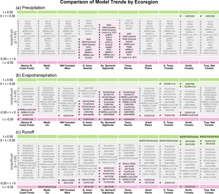
Only 19 out of 87 component estimates exhibit statistically dominated Northwestern Forested Mountains and Northern
significant CONUS average domain trends, evaluated with Forests ecoregions (Fig. 5d), where annual peak SWE val-
Sen’s slope, from 1982 to 2010 (Fig. 4). Within most com- ues exceed estimated snowpack in the remaining ecoregions
ponents, one or more data sets produced a significant slope by up to 700 % (Fig. B2). Of primary interest is the North-
western Forested Mountains ecoregion that contains the
that is contradicted by one or more data sets. For example,
the R estimates from LSMs GLDAS-CLM, JRA-55/SiB, and snowmelt-dominated regimes of the Rocky, Sierra Nevada,
ERA5/H-TESSEL each show a significant negative trend in and Cascade mountain ranges that are strong contributors
annual values across the CONUS over the 1982–2010 period. to water supply for population centers such as Denver, Los
Conversely, the NCEP–DOE/Eta-Noah LSM shows a signif- Angeles, San Francisco, Portland, and Seattle. In this ecore-
icant positive trend over the same period, and the remaining gion, modeled estimates of monthly mean SWE storage vary
data sets, a mix of hydrologic and reanalysis models, show by 76 % to 84 %, equating to median equivalent water depth
no significant trend. While the NCEP–DOE reanalysis pre- standard deviations as high as 48 mm per month.
cipitation trend matches that of the NCEP–DOE forced Eta- SM(e) estimate uncertainty (Fig. 5e) is greatest, 66 %–
Noah, model estimates of SWE indicate a significant nega- 96 %, in arid western ecoregions, though other regions fall
tive trend. within a 64 %–83 % uncertainty range. SM(v) shows lower
overall uncertainty (Fig. 5f), with less dramatic differences
between regions, ranging from 36 % to 57 %, with the great-
3.2 Ecoregions est uncertainty (44 %–57 %) in central and eastern CONUS
ecoregions. As mentioned previously, uncertainty in SM es-
3.2.1 Magnitude variability timates, most importantly SM(e), is strongly influenced by
model-defined root zone soil thickness. Spatial differences
Uncertainty in modeled hydrologic component estimates in in SM(e) uncertainty measured as CV, therefore, are pro-
each ecoregion is presented in terms of CV (Fig. 5) and σ nounced in regions with lower water content because CV, a
(Appendix A). Ecoregions are organized from west to east measure of relative variability, is more strongly affected by
within each figure. Results and discussion of uncertainty are magnitude differences. Because the range of values is con-
focused primarily on CV due to the disparity in annual wa- strained from 0 to 1 in m3 per cubic meter, uncertainty in
ter flux between regions. By component, P and ET estimates SM(v) is less influenced by spatial variability in soil water
demonstrate lower uncertainty compared to other hydrologic magnitudes and is therefore a better measure for understand-
components (Fig. 5a, b). P estimates typically range in me- ing regional soil water estimate disagreement. Following this
dian uncertainty from 5 % to 14 % in the eastern CONUS logic, SM(v) uncertainty is greater in Tropical Wet Forests,
and 11 % to 21 % in the western CONUS. P uncertainty is Northern Forests, and Great Plains ecoregions, with an av-
highest in mountainous regions with more variable topogra- erage CV of 53 % compared to an average of 42 % for the
phy (e.g., Northwestern Forested Mountains and Temperate remaining ecoregions.
Sierras) and lowest in more humid, topographically homoge-
neous regions (e.g., Eastern Temperate Forests). 3.2.2 SWE accumulation and ablation
The median uncertainties of ET estimates typically range
from 13 % to 22 % in the eastern CONUS ecoregions and Timing of SWE estimates is presented in terms of relative
14 % to 26 % in the western CONUS. Uncertainty is great- timing (Figs. B3 and B4). Figures are divided by Northern
est along the Pacific coast and northerly ecoregions and arid Forests and Northwestern Forested Mountains ecoregions,
and semiarid ecoregions that are heavily influenced by an- trends of accumulation and ablation, and early and late pe-
thropogenic water use. Of the four largest ecoregions (Ta- riods. Negative (positive) values in purple (green), identify
ble 2), Northwestern Forested Mountains and North Amer- models for which accumulation or ablation begins more than
ican Deserts demonstrate mean uncertainties of 21 % and 1 month earlier (later) than the mean of other data sets. Dis-
19 %, respectively, and the Great Plains and Eastern Tem- tributions of relative timing by year are presented in Fig. B3
perate Forests demonstrate mean uncertainties of 14 % each. and summarized as the percentage of years that are positive
https://doi.org/10.5194/hess-25-1529-2021 Hydrol. Earth Syst. Sci., 25, 1529–1568, 2021
1538                    S. Saxe et al.: A comparison of publicly available, CONUS-extent hydrologic component estimates

Figure 4. Forest plot of interannual (water year) component estimate Sen’s slope from 1982 to 2010 for components of precipitation (P ),
evapotranspiration (ET), snow water equivalent (SWE), soil moisture in units of equivalent water depth (SM(e)), and soil moisture in units of
volumetric water content (SM(v)). Insignificant trends (p>0.05) are gray. Significant trends are colored based on direction, where negative
trends are gold and positive trends are green. Data sets without complete data during the study period are represented with hollow points,
and the temporal extent is noted under “Years in Period” column.

Hydrol. Earth Syst. Sci., 25, 1529–1568, 2021                                              https://doi.org/10.5194/hess-25-1529-2021
S. Saxe et al.: A comparison of publicly available, CONUS-extent hydrologic component estimates                                          1539

Figure 5. Box plots of uncertainty, measured as annual coefficient of variation (CV), between component estimates at 10 ecoregions. CV
distributions are subdivided into late and early periods, i.e., 1985–1999 and 2000–2014. Box lower limits, midlines, and upper limits represent
the 25th, 50th (median), and 75th percentiles, respectively, of the associated data. Whiskers represent 1.5 times the interquartile range. Box
colors denote the ecoregion and correspond to the map colors in Fig. 1. Components displayed are precipitation (P ), evapotranspiration (ET),
runoff (R), snow water equivalent (SWE), soil moisture in units of equivalent water depth (SM(e)), and soil moisture in units of volumetric
water content (SM(v)). Results for SWE uncertainty are omitted for ecoregions with limited annual snowpack.

or negative in Fig. B4. In both ecoregions, uncertainty among             much earlier ablation times, often 1–2 months after the mean
data sets is greater in ablation timing than accumulation tim-            antecedent month (Fig. B3). Uncertainty in ablation timing is
ing, and overall uncertainty is greater in the Northwestern               typically much higher in the Northwestern Forested Moun-
Forested Mountains ecoregion than in the Northern Forests.                tains ecoregion than in the Northern Forests. The Daymet,
   Relative timing between models can be similar between                  ERA5-Land/H-TESSEL, Livneh-VIC, NLDAS2-VIC, and
ecoregions (Figs. B3a and B4), especially regarding accu-                 SNODAS models commonly estimate a later start to ablation
mulation. For instance, the AMSR-E/Aqua RS and NHM-                       than the remaining models.
MWBM CM consistently show later accumulation start dates                     Models that predict earlier (later) accumulation timing
than other data sets in both ecoregions, while the ERA5-                  and later (earlier) ablation timing represent longer (shorter)
Land/H-TESSEL, JRA-55/SiB, and SNODAS models esti-                        periods of growing or available snowpack (Fig. B4). The
mate earlier accumulation dates. Conversely, the JRA-25/SiB               ERA5-Land/H-TESSEL, Livneh-VIC, and SNODAS mod-
and TerraClimate models show different trends in accumula-                els estimate longer snowpack periods than other models in
tion timing between regions with earlier SWE accumulation                 both ecoregions. The AMSR-E/Aqua, JRA-55/SiB, NHM-
in Northern Forests but later accumulation in Northwestern                PRMS, and TerraClimate models estimate longer snow-
Forested Mountains.                                                       pack periods in only one ecoregion. The NCEP-NARR/Eta-
   Regarding ablation, outliers are much more common when                 Noah, NLDAS2-Mosaic, and NLDAS2-Noah models esti-
comparing models (Figs. B3b and B4). For example, the                     mate shorter snowpack periods in the Northern Forests ecore-
Daymet model consistently estimates a much later start                    gion while the GLDAS-CLM and JRA-25/SiB models esti-
of spring ablation while the Eta-Noah models driven with                  mate shorter snowpack periods in the Northwestern Forested
NCEP–DOE and NCEP-NARR reanalyses typically estimate                      Mountains ecoregion.

https://doi.org/10.5194/hess-25-1529-2021                                               Hydrol. Earth Syst. Sci., 25, 1529–1568, 2021
1540                  S. Saxe et al.: A comparison of publicly available, CONUS-extent hydrologic component estimates

   Attributing the relative timing of SWE to model type is        sets show no significant trend (Fig. B5d). Trend agreement is
difficult at the monthly scale. LSMs estimate both earlier        better among SM data sets (mean u = 0.25), though higher
and later accumulation and ablation antecedences, and the         u is noted in the Northwestern Forested Mountains, North
two WBMs in this study show opposing timing trends. Simi-         American Deserts, and Northern Forests and is caused by
larly, grouping by organization does not yield significant sim-   conflicting negative and insignificant τ values. Ecoregions
ilarities. For example, the timing of NLDAS2-driven LSMs          with low u typically show no significant τ values in SM data
from the National Aeronautics and Space Administration            sets, except for the Southern Semiarid Highlands where most
(NASA) is dissimilar from that of the MERRA-2-driven and          data sets show a significant negative τ .
MERRA-Land-driven CLSM, which are also from NASA.                    Generally, τ disagreement is highest in the North Amer-
Forcing data also do not yield useful information for identi-     ican Deserts and Northern Forests ecoregions and lowest
fying controlling variables. Only the NLDAS2-driven mod-          in the Mediterranean California, Eastern Temperate Forests,
els from NASA tend to all show later (earlier) accumula-          Marine West Coast Forest, and Tropical Wet Forests ecore-
tion (ablation) timing. Even the Eta-Noah LSMs, driven by         gions. Trend disagreement is almost always caused by con-
the NCEP–DOE reanalysis and the corresponding higher-             flicting negative and insignificant trends, indicating that dis-
resolution version for North America NCEP-NARR show               agreement is due to the occurrence, and not the direction,
different relative timing values in both ecoregions.              of the trend. That is to say, higher u values are caused by
                                                                  disagreement over whether there is or is not a significant
3.2.3   Trend                                                     trend present in the data, as opposed to higher u values be-
                                                                  ing caused by disagreement between significant negative and
Interannual trend analyses performed with the Mann–               significant positive trends.
Kendall trend test (τ ) over water years 1982–2010 show
varying degrees of agreement and disagreement between             3.2.4   Correlation with remote sensing
ecoregions. Figures showing explicit distributions of trends
with model names are supplied in the appendix (Fig. B5).          Spearman’s rho (ρ) correlation was calculated for all hydro-
Model disagreement in trend direction is quantified using the     logic models and reanalysis data sets against remote sens-
unalikeability coefficient (u; Fig. 6), with 0 and 1 being com-   ing products with 48 or more months of intersecting tempo-
plete agreement and disagreement, respectively.                   ral extents (Fig. 7; Table 3). Precipitation data sets (Fig. 7a,
   Precipitation estimates demonstrate the lowest u, showing      b), correlated against the GPCP-v3 and TMPA-3B43 prod-
no (u = 0) to low (u = 0.13) disagreement in eight ecore-         ucts, show high correlation compared against 13 data sets
gions where data sets show no significant τ (Fig. B5a). Dis-      (ρ = 0.93–0.99) with no statistically insignificant values.
agreement is higher in North American Deserts and Temper-         Variability in P estimate correlations are low (± 0.01–0.09).
ate Sierras ecoregions (u = 0.41–0.49) where most data sets       ET data sets correlated against the MOD16-A2 and SSE-
show a negative τ , and all data sets show a negative τ in the    Bop products (Fig. 7c, d) show poorer correlation in west-
Southern Semiarid Highlands. Coefficient u is higher among        ern ecoregions, with mean ρ ranging from 0.59 to 0.91. Ex-
ET data sets than P data sets, averaging 0.21 across ecore-       treme cases are found when correlating against MOD16-
gions, notably in the North American Deserts and Marine           A2 in North American Deserts (ρ = −0.28) and SSEBop
West Coast Forest ecoregions (u = 0.46 and 0.53), where           in Mediterranean California (ρ = 0.25), where four data sets
negative and insignificant τ values are present (Fig. B5b).       show insignificant ρ. The exception in the western CONUS
All data sets identify negative ET τ in the Southern Semi-        is in Northwestern Forested Mountains, where models cor-
arid Highlands and Temperate Sierras. Data sets show pos-         relate against both RS data sets well (MOD16-A2 ρ = 0.91
itive, negative, and insignificant τ in the Eastern Temperate     and SSEBop ρ = 0.89). Correlation against both products is
Forests (u = 0.31) and Northern Forests (u = 0.53). Runoff        high in eastern ecoregions, ranging from ρ = 0.88 to 0.96,
data sets show the most consistent spatial distribution of u>0    with standard deviation decreasing as ρ increases.
across the study ecoregions. Disagreement in the western             SWE data sets correlated against the AMSR-E/Aqua prod-
ecoregions is caused by conflicting negative and insignif-        uct are highlighted for the Northwestern Forested Mountains
icant Rτ (Fig. B5c), with the greatest u in the Southern          and Northern Forests ecoregions (Fig. 7e). Modeled esti-
Semiarid Highlands (u = 0.50) and Temperate Sierras (u =          mates correlate better in the Northwestern Forested Moun-
0.49). Eastern ecoregion τ is generally caused by conflicting     tains (ρ = 0.91) than Northern Forests (ρ = 0.80). SM data
positive, negative, and insignificant τ values (u = 0.26–44).     sets show worse and more variable ρ against remote sens-
Ecoregions with good agreement (u = 0–0.35) are generally         ing products ESA-CCI and SMOS-L4 (Fig. 7f, g) than
due to most data sets showing no significant trend.               other components. At the CONUS scale, estimates corre-
   SWE data sets, limited in this study to the Northwestern       late very poorly against the ESA-CCI product (ρ = 0.17) and
Forested Mountains and Northern Forests, show disagree-           only moderately well against SMOS-L4 (ρ = 0.68). Gen-
ment, i.e., u = 0.42 and 0.40, respectively, mostly caused        erally, correlation is best in the Mediterranean California
by conflicting negative and insignificant τ , though most data    and Eastern Temperate Forests ecoregions (ρ = 0.74–0.92).

Hydrol. Earth Syst. Sci., 25, 1529–1568, 2021                                      https://doi.org/10.5194/hess-25-1529-2021
Table 3. Spearman’s rho (ρ) correlation of monthly hydrologic model and reanalysis data set estimates against remote sensing products quantifying hydrologic components precipitation
(P ), evapotranspiration (ET), snow water equivalent (SWE), and soil moisture (SM). Correlation was calculated at 10 ecoregions and at the CONUS extent. The number of modeled
data sets correlated against remote sensing products is shown as (n = X) for each column. Mean and standard deviation (σ ) of ρ are provided for each ecoregion and remote sensing
products as ρ ± σ . Counts of statistically insignificant correlations (Y ) are denoted when n>0 as (Y ). SM combines data sets produced in units of equivalent water depth (SM(e) in
text) and volumetric soil moisture water content (SM(v) in text). Correlation of SWE products is included only for regions of high annual mean SWE storage. Hydrologic model and
reanalysis data sets (Table 1) used in each column are listed in the footnotes.
P AET SWE RZSM
https://doi.org/10.5194/hess-25-1529-2021
GPCP-v3a TMPA-3B43b MOD16-A2c SSEBopc AMSR-E/Aquad ESA-CCIe SMOS-L4f
Ecoregion (n = 15) (n = 14) (n = 15) (n = 15) (n = 18) (n = 15) (n = 13)
Marine West Coast Forest 0.99 ± 0.01 0.99 ± 0.01 0.82 ± 0.18 0.80 ± 0.19 –g 0.72 ± 0.09 0.78 ± 0.09
Mediterranean California 0.98 ± 0.01 0.97 ± 0.02 0.71 ± 0.20 0.25 ± 0.42 (4) –g 0.79 ± 0.13 0.92 ± 0.04
Northwestern Forested Mountains 0.97 ± 0.05 0.96 ± 0.05 0.91 ± 0.06 0.89 ± 0.08 0.91 ± 0.07 0.58 ± 0.10 0.27 ± 0.12 (2)
North American deserts 0.95 ± 0.05 0.94 ± 0.05 −0.28 ± 0.17 (4) 0.81 ± 0.13 –g 0.61 ± 0.18 0.28 ± 0.11 (2)
Southern Semiarid Highlands 0.97 ± 0.04 0.96 ± 0.05 0.67 ± 0.17 0.64 ± 0.17 –g 0.63 ± 0.20 0.79 ± 0.16
Temperate Sierras 0.97 ± 0.04 0.96 ± 0.04 0.59 ± 0.15 0.68 ± 0.18 –g 0.51 ± 0.19 0.43 ± 0.21 (1)
Great Plains 0.99 ± 0.02 0.98 ± 0.01 0.92 ± 0.02 0.93 ± 0.03 –g 0.62 ± 0.15 0.69 ± 0.06
Eastern Temperate Forests 0.95 ± 0.09 0.94 ± 0.07 0.96 ± 0.03 0.94 ± 0.03 –g 0.74 ± 0.10 0.83 ± 0.08
Northern Forests 0.96 ± 0.03 0.93 ± 0.02 0.94 ± 0.03 0.94 ± 0.02 0.80 ± 0.03 0.44 ± 0.08 0.12 ± 0.21 (10)
Tropical Wet Forests 0.97 ± 0.03 0.96 ± 0.03 0.88 ± 0.05 0.88 ± 0.09 –g 0.40 ± 0.19 (1) 0.57 ± 0.16
CONUSh 0.94 ± 0.07 0.91 ± 0.06 0.95 ± 0.02 0.95 ± 0.03 0.91 ± 0.03 0.17 ± 0.05 (4) 0.68 ± 0.09
a CMAP enhanced and standard, Daymet, ERA5, ERA5-Land, GPCC, gridMET, Livneh et al. (2013), Maurer et al. (2002), MERRA-2, MERRA-Land, NCEP–DOE, NLDAS2, PRISM, and UoD-v5.
b CMAP enhanced and standard, Daymet, ERA5, ERA5-Land, GPCC, gridMET, Livneh et al. (2013), MERRA-2, MERRA-Land, NCEP–DOE, NLDAS2, PRISM, and UoD-v5.
c CSIRO-PML, ERA5-Land/H-TESSEL, GLDAS-CLM, GLEAM-v3.3a and v3.3b, MERRA-2 and MERRA-Land/CLSM, NHM-MWBM and NHM-PRMS, NLDAS2-Mosaic, NLDAS2-Noah, NLDAS2-VIC,
Reitz et al. (2017), TerraClimate, and VegET.
d CanSISE, Daymet, ERA5-Land/H-TESSEL, GLDAS-CLM, JRA-25 and JRA-55/SiB, Livneh-VIC, MERRA-2 and MERRA-Land/CLSM, NCEP–DOE and NCEP-NARR/Eta-Noah, NHM-MWBM and
NHM-PRMS, NLDAS2-Mosaic, NLDAS2-Noah, and NLDAS2-VIC, SNODAS, and TerraClimate.
e CPC, ERA5-Land and ERA5/H-TESSEL, GLEAM-v3.3a and v3.3b, JRA-25 and JRA-55/SiB, MERRA-2/CLSM, NHM-MWBM and NHM-PRMS, NLDAS2-Mosaic, NLDAS2-Noah and NLDAS2-VIC,
TerraClimate, and VegET.
f CPC, ERA5-Land and ERA5/H-TESSEL, GLEAM-v3.3a and v3.3b, JRA-55/SiB, MERRA-2/CLSM, NHM-PRMS, NLDAS2-Mosaic, NLDAS2-Noah, and NLDAS2-VIC, TerraClimate, and VegET.
g Regions omitted.
S. Saxe et al.: A comparison of publicly available, CONUS-extent hydrologic component estimates
h Calculated from data sets spatially aggregated by weighted area mean at the CONUS extent (Fig. 1) and not as a mean of individual ecoregion ρ estimates above.
Hydrol. Earth Syst. Sci., 25, 1529–1568, 2021
15411542 S. Saxe et al.: A comparison of publicly available, CONUS-extent hydrologic component estimates
Figure 6. Bar plots summarizing the disagreement in Mann–Kendall trend (τ ) direction using the unalikeability coefficient (u) after cate-
gorizing τ as significant negative trend, significant positive trend, or no significant trend for 10 ecoregions from 1982 to 2010. Trends were
assumed to be significant if pc, maximum possible u is approximately 0.71 (dotted red line). Text to the
right of each bar shows, in order, the u value and the number of data sets showing the negative, insignificant, or positive trend. Bars are color
matched to ecoregion colors from Fig. 1 and are ordered from west (top) to east (bottom). Results are provided for water balance components
of precipitation (P ), evapotranspiration (ET), runoff (R), snow water equivalent (SWE), and soil moisture (SM) in units of either equivalent
water depth or volumetric water content.
Correlation is worst in Northwestern Forested Mountains, eastern ecoregions of the Great Plains and Eastern Temper-
North American Deserts, and Northern Forests (ESA-CCI ate Forests (11 %, 19 %, 29 %, and 31 % of the CONUS area,
ρ = 0.44–0.61; SMOS-L4 ρ = 0.12–0.28). Explicit distribu- respectively).
tions of correlation for each data set by ecoregion are pro- Of these larger domains, water budget Rε values in the
vided in Fig. B6. eastern ecoregions show much lower variability (Table 4),
with the Great Plains and Eastern Temperate Forests yield-
3.2.5 Case study – impact of model selection on water ing σ values of 18.2 percentage points and 14.3 percent-
budget imbalances age points, respectively, and medians of 3.9 % and −0.4 %,
respectively. Similarly, the 10th and 90th percentiles (P10
A case study calculating 2925 10 year water budgets (WY and P90) are −23.2 % and 23.6 % for the Great Plains and
2001–2010) using 15 P , 15 ET, and 13 R estimates for each −19.9 % and 17.2 % for the Eastern Temperate Forests. In
of the 10 ecoregions was performed to demonstrate quantita- contrast, the major western ecoregions exhibit much higher
tively how model selection can affect research results. Each variability, with Northwestern Forested Mountains and North
water budget was solved for a relative imbalance (Rε) with American Desert σ values of 45.6 % and 27.0 %, respec-
Eq. (7), which estimated the model error as a fraction of total tively, and medians of −6.7 % and 4.7 %, respectively. P10
water flux in P . and P90 are higher than eastern regions as well, yielding
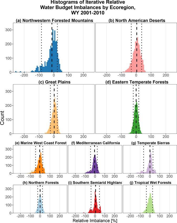
Histograms of the results, overlain with box plots (Fig. 8), −83.3 % and 23.8 % for the Northwestern Forested Moun-
demonstrate the range and distribution of potential water tains and −33.2 % and 36.6 % for the North American
budget Rε values. In most ecoregions, Rε values exhibit an Deserts. Smaller ecoregions (Fig. 8e–j) yield similar spatial
approximately normal distribution. The following four ecore- trends in variability, with the eastern Northern Forests ecore-
gions dominating the area of the CONUS (Fig. 8a–d), con- gion showing lower σ and P10 and P90 than the western Ma-
stituting 90 % of the CONUS area (Table 2), are the focus rine West Coast Forest and Mediterranean California ecore-
of these results: the western ecoregions of the Northwest- gions.
ern Forested Mountains and North American deserts and the
Hydrol. Earth Syst. Sci., 25, 1529–1568, 2021 https://doi.org/10.5194/hess-25-1529-2021S. Saxe et al.: A comparison of publicly available, CONUS-extent hydrologic component estimates 1543
Figure 7. Spearman’s rho (ρ) correlation values of hydrologic model and reanalysis data set component estimates against remote-sensing-
derived products for components of precipitation (P ), evapotranspiration (ET), soil moisture in units of both equivalent water depth (SM(e))
and volumetric water content (SM(v)), and snow water equivalent (SWE). The title of each sub-plot (e.g., Fig. 7a) provides the hydrologic
component (e.g., P ) and the remote sensing product against which the data set was correlated (e.g., GPCP-v3). Statistically significant ρ
values (p0.05) are shown as black squares. Horizontal bars within each
ecoregion denote mean ρ. Point and bar colors correspond to ecoregions, as shown in Fig. 1. Each point or square corresponds to a single
modeled data set, with points sorted by descending ρ value. More detailed information can be found in Fig. B6.
The Northwestern Forested Mountains region, accounting uncertainty of ET estimates in arid, semiarid, and mountain-
for 11 % of the CONUS area, is unique among ecoregions ous regions, as well as lower uncertainty in eastern regions.
in this study. It exhibits the greatest magnitude of variability Haddeland et al. (2011) found that LSMs underestimate R
in iterative water budget Rε, P10–P90 Rε ranges, skewness partitioning relative to global hydrologic models (not used in
(−1.6), and kurtosis (3.7). Furthermore, the difference be- this paper). Here, we find that LSMs are more likely to esti-
tween the ensemble water budget Rε and median iterative mate greater R than either WBMs or CMs. Xia et al. (2012a,
water budget Rε is greater than any other ecoregion (−6.3 b) noted greater model disagreement in R estimates between
points). several LSMs in the northeastern and western mountainous
regions of the CONUS. This paper, using CV as a measure of
relative uncertainty, alternatively shows that modeled runoff
4 Discussion uncertainty is higher in the arid and semiarid regions of the
western CONUS where annual R rates are lower.
Results of model comparisons demonstrate the effect
Previous analyses of modeled SWE estimates focused
that model disagreement can have on both regional- and
largely on the validation of winter snowpack magnitudes
continental-scale research. Comparisons of P estimates
against the SNODAS model or on the timing of accumulation
agree with previous findings (Derin and Yilmaz, 2014; Guir-
and ablation periods. Broxton et al. (2016) found that LSMs
guis and Avissar, 2008; Sun et al., 2018), noting increased
estimated earlier ablation timing than observational measure-
uncertainty between products in regions of complex topog-
ments, in contrast with the results of Essery et al. (2009) and
raphy. ET comparisons showed that LSMs are more likely to
Rutter et al. (2009), who noted later timing in LSMs. Our re-
produce lower annual ET than CMs and WBMs, similar to re-
sults indicate the alternative argument that neither snow ac-
sults found by Mueller et al. (2011), and that model disagree-
cumulation nor ablation timing can be accurately attributed
ment is higher in Pacific regions, similar to the comparison
solely to model design and note differences in relative timing
and validation of MOD16-A2, NLDAS2-Noah, and ALEXI
of as much as 2 months between LSMs. In contrast to the ar-
by Carter et al. (2018). However, this paper finds some differ-
guments by Murdryk et al. (2015) and Broxton et al. (2016),
ences from the work of Carter et al. (2018) and notes a higher
https://doi.org/10.5194/hess-25-1529-2021 Hydrol. Earth Syst. Sci., 25, 1529–1568, 2021You can also read