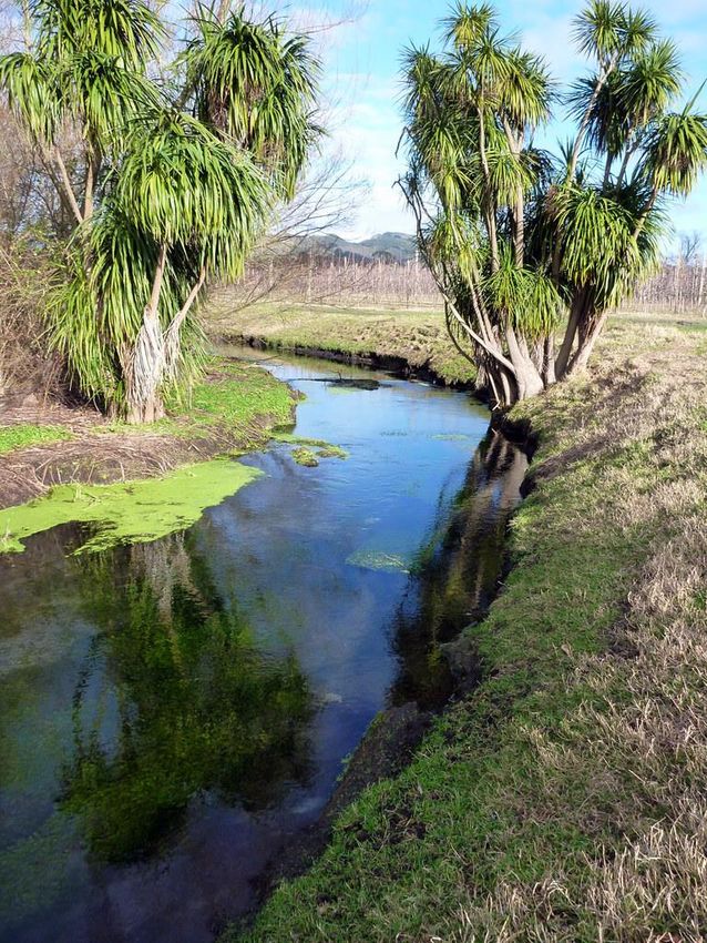
Heretaunga Springs Gains and groundwater on the Heretaunga Plains losses of stream - Hawke's Bay Regional Council
←
→
Page content transcription
If your browser does not render page correctly, please read the page content below
Heretaunga Springs
Gains and losses of stream flow to
groundwater on the Heretaunga Plains
June 2018
HBRC Report No. RM18-13 – 4996

Environmental Science - Hydrology

Heretaunga Springs
Gains and losses of stream flow to
groundwater on the Heretaunga Plains
June 2018
HBRC Report No. RM18-13 – 4996

…………………………………………………………………….

Prepared By:
Thomas Wilding

Reviewed By:
Stephen Swabey

Approved By:
Iain Maxwell – Group Manager – Resource Management

.
Contents
Executive summary ....................................................................................................................... 5

1       Introduction ........................................................................................................................ 6
        1.1      Scope ................................................................................................................................... 6
        1.2      Flow gains and losses .......................................................................................................... 7
        1.3      Hydrogeology ...................................................................................................................... 8
        1.4      Climate .............................................................................................................................. 10

2       Methods............................................................................................................................ 11
        2.1      Locating Springs and Measuring Flow Gains..................................................................... 11
        2.2      Measuring Flow Losses ..................................................................................................... 18

3       Results .............................................................................................................................. 18
        3.1      Ngaruroro.......................................................................................................................... 18
        3.2      Lower Tukituki................................................................................................................... 29
        3.3      Tutaekuri ........................................................................................................................... 33
        3.4      Paritua-Karewarewa ......................................................................................................... 36
        3.5      Awanui .............................................................................................................................. 42
        3.6      Louisa and Te Waikaha ..................................................................................................... 44
        3.7      Irongate and Upper Southland ......................................................................................... 47
        3.8      Karamu .............................................................................................................................. 52
        3.9      Mangateretere .................................................................................................................. 61
        3.10 Raupare ........................................................................................................................... 65
        3.11 Maraekakaho .................................................................................................................... 69
        3.12 Waitio             ........................................................................................................................... 71
        3.13 Tutaekuri-Waimate ........................................................................................................... 72
        3.14 Other small streams .......................................................................................................... 77

4       Synthesis of results - springs of the Heretaunga Plains ........................................................ 81

5       Acknowledgements ........................................................................................................... 83

6       References ........................................................................................................................ 84

Appendix A           Spring locations and attributes ............................................................................ 87

Appendix B           Stable Isotope data ............................................................................................. 90

Heretaunga Springs
Heretaunga Springs
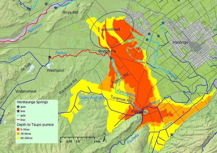
Executive summary

Springs are the link between groundwater use and stream flows. Managing water use for the protection of
stream ecosystems benefits from an understanding of spring inputs, because most water use on the
Heretaunga Plains is from groundwater. This groundwater is used for irrigation, industry and drinking water.

Springs of the Heretaunga Plains were investigated to help inform flow-ecology investigations and
groundwater modelling. This report is primarily a technical reference, focussing on the location of flow gains
and losses, as well as the methods used to quantify them. Readers looking for a general overview are directed
to Section 1 (Introduction) and Section 4 (Synthesis). The results (Section 3) provide details for specific sub-
catchments.

The location of springs was investigated using a range of methods, starting with aerial photographs to narrow
down the areas of interest. Spring locations and property access were then discussed with landowners before
walking or kayaking the length of targeted streams. Measuring electrical conductance often revealed spring
inputs that were sourced from larger catchments with less dissolved ions (e.g. Ngaruroro water). More
quantitative surveys included flow gauging and longitudinal surveys of electrical conductance. Stable
isotopes provided further insight into the source of spring water. Loss of flow to groundwater was estimated
from the difference in gauged flow between sites.

The investigation identified 64 springs throughout the Heretaunga Plains, which represents the largest
number of springs documented to date. This report does not provide a complete list of springs, instead
capturing the major gains and major losses for sub-catchments of the Heretaunga plains. Most of the major
flow losses to groundwater have been described previously, including losses from the Ngaruroro River that
continue through dry summers when the aquifer receives little recharge from local rainfall. During these
times, flow losses from the Ngaruroro River are vital for sustaining spring flow to the Raupare, Tutaekuri-
Waimate and Waitio streams. Likewise, flow losses from the Tutaekuri River probably sustain springs in
Moteo Valley (Tutaekuri-Waimate headwaters).

This investigation located large springs that contribute more than half of the low flow to the Karamu Stream.
The Tukituki River was probably the main source of spring inflows direct to the Karamu Stream and to the
Mangateretere Stream under low flow conditions on 3/3/2015. This changed in winter (23/8/2017), when
isotope results indicated that nearly half of the groundwater originated from the Ngaruroro River.

These investigations also revealed a tufa coating (calcite deposited from flowing water) on the bed of the
Paritua Stream. The Paritua Stream has run dry in summers past. This stream loses flow to groundwater
where it crosses unconfined alluvial gravels upstream of Bridge Pa. The tufa coating is important in extending
the length of flowing stream because it probably reduces the rate of flow loss to groundwater.

An extensive area of shallow Taupo pumice sands contributes groundwater to several streams, including the
Karewarewa, Louisa and Awanui. Little is known of the groundwater in this pumice sand layer because it is
not used for irrigation or domestic water supply. However, it may be an important source of flow and
nutrients for these streams, and hence deserves further investigation.

This report goes beyond describing where streams are, to also describe their location in the past. For
example, the Hawke’s Bay earthquake of 1931 changed the drainage patterns of the Heretaunga Plains,
including shifting the Paritua outflow from Irongate Stream to Karewarewa Stream. On alluvial plains such as
the Heretaunga, floods and channel processes generate a naturally dynamic river network. In addition to
these natural processes, people have made significant changes to the stream network to reduce flooding and
drain soils for horticulture.

Heretaunga Springs                                                                                      5
1       Introduction
1.1     Scope
Springs link groundwater use to surface water flows. Managing water use for the protection of stream
ecosystems benefits from a good understanding of spring contributions to the stream, because most of the
water use on the Heretaunga Plains is from groundwater (HBRC, 2014). Loss of river flow to groundwater is
important for the same reasons.

This report is primarily a technical reference, focussing on the location of springs and flow losses, as well as
the methods used to quantify them. These investigations were initiated for flow-ecology studies. In
particular, the spatial oxygen model was based on a hydrogeomorphic template that described flow patterns
across the Heretaunga Plains (Wilding, 2016). Additionally, the MODFLOW surface water-groundwater
models were constructed in part using the spring information presented here (Rakowski, in prep 2018).

This report is not intended to provide a complete list of springs on the Heretaunga plains. It is intended to
capture the major gains and losses for sub-catchments of the Heretaunga plains (sub-catchments as defined
by the Section 3 sub-headings). Investigations for this report focused on finding the springs that feed spring-
dominated streams, with less effort spent on locating springs feeding runoff-dominated streams. All streams
are fed from groundwater, including those that run dry. All streams also receive some degree of fast rainfall-
runoff. The distinction arises between streams where spring inflows dominate the flow for much of the year
(spring-dominated), and streams where most of the flow arrives as rainfall-runoff, or quickflow (runoff-
dominated). This simple dichotomy between spring and runoff dominated streams is adequate for this report.
However, it is a simplification of the many possible classes of flow regime (Pyne et al., 2016).

Within the spring-dominated streams, more effort was put into finding springs that may be fed from areas
outside the stream’s surface-water catchment (e.g. Raupare springs originating from Ngaruroro flow losses),
as these are more difficult to quantify from conventional investigations (e.g. catchment water-balance
models). Tributaries that contributed a larger proportion of mainstem flows were further prioritised. Losses
from stream flow to groundwater aquifers were also a priority, including their location and magnitude.
Springs emerging offshore, or within estuaries, were not investigated.

The type of information that is presented for each sub-catchment depends on what methods were known
and available at the time. Some methods were developed over the course of this investigation, hence were
not applied consistently across the sub-catchments.

Information from wells (e.g. lithology, water elevation, chemistry) is critical for understanding how
groundwater and surface water interact. Information from springs (location, elevation, flow, chemistry)
provides another piece of the puzzle. Springs offer a different perspective on surface water-groundwater
interactions, compared to wells. The springs reflect groundwater processes closer to the surface, with a larger
outflow that integrates groundwater processes over a larger area of the aquifer, compared to a single well.
Well samples offer less spatial representation, but better specificity of results, representing a known location
and depth within the aquifer. Patterns in spring location, elevation, flow and chemistry are therefore
complementary to groundwater well information for developing conceptual models of surface-groundwater
interactions. Information from this report is therefore intended to aid refinements of the conceptual models
for surface-groundwater interactions for the Heretaunga Plains.

In describing the pattern of springs and streams, it is also important to understand their history. For example,
the Hawke’s Bay earthquake of 1931 changed the drainage patterns of the Heretaunga Plains, including
shifting the Paritua outflow from Irongate Stream to Karewarewa Stream. On alluvial plains such as the
Heretaunga, floods and channel processes generate a naturally dynamic river network (Hauer et al., 2016;

Heretaunga Springs                                                                                      6
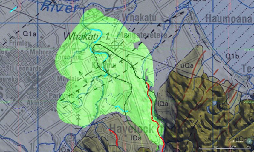
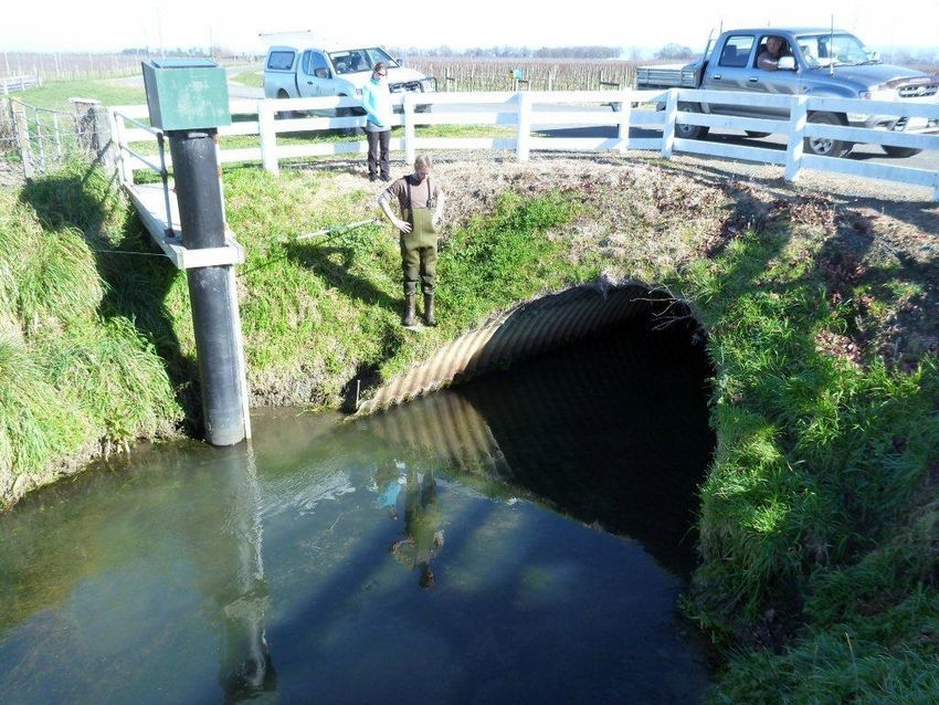
Wakefield et al., 2012). In addition to these natural processes, people have made significant changes to the
stream network in order to reduce flooding and drain soils for horticulture (HBRC, 2004). This report
therefore goes beyond describing where streams are, to also describe their location in the past.

1.2     Flow gains and losses
Just as streams can gain flow from groundwater, via springs, the reverse can also occur with a net loss of
stream flow to groundwater. As groundwater levels drop, spring flow diminishes (Figure 1-1). If groundwater
levels continue to drop below the streambed elevation, then the same hole through which spring water
emerged can become a hole through which water is lost from the stream to groundwater (when there is
surface water to be lost). For many springs, the outflow does not stop, reflecting groundwater levels that
remain above stream level (e.g. Raupare spring). Conversely, there are some streams where we have only
ever measured a loss (e.g. Ngaruroro upstream of Fernhill).

Considering the full length of a stream, dry sections can transition to gaining sections where the streambed
intersects the groundwater level (Figure 1-1). If layers of gravel connect the stream to groundwater, then
spring inflows will be more diffuse/spread out. In contrast, the more discrete, point-springs with boiling sands
occur where clay confining-layers separate the stream from the groundwater, and the connection to the
stream is via discrete holes in the confining layer. Those holes can take the form of gravel and sand
interspersed through the confining layer (Harper & Hughes, 2009). The length of diffuse springs can increase
during winter when groundwater levels are higher, compared to the fixed location of point-springs.

Between the two extremes of a point spring emerging through a discrete hole, and a diffuse spring emerging
through unconfined gravels, exists a gradation of intermediate springs. For example, sand and gravel or tree
roots interwoven through the thin edge of the confining clays can create a series of small point springs that
together form a relatively diffuse input to stream flow.

Heretaunga Springs                                                                                      7

diffuse springs

                                                              point spring

                    recharge      diffuse springs
    winter                      (longer in winter)
    groundwater level
                                                                                    Point spring
    groundwater level
    summer

                                     gravel aquifer

Figure 1-1: Diffuse and point springs. The length of diffuse springs can increase during winter when groundwater
levels are higher, compared to the fixed location of point-springs, as demonstrated in this stylised diagram. Example
photographs from the Raupare catchment show diffuse springs (left) and a point spring (right).

1.3        Hydrogeology
The Heretaunga Plains have been built up by the outflow of gravel from the three major rivers – Ngaruroro,
Tukituki and Tutaekuri (Dravid & Brown, 1997; Harper & Hughes, 2009; Lee et al., 2014). The bedload of
gravel that was eroded from the ranges (e.g. Ruahine, Kaweka) exceeded the carrying capacity of these rivers
as they crossed the plains. Deposited gravel has pushed the river into new flowpaths and, in doing so,
gradually spread the sediment across the plains. Old flowpaths eventually became buried (Figure 1-2). Some
of these palaeochannels have larger spaces between the gravel and cobbles, providing a preferential
flowpath for faster movement of groundwater.

Sea level rise between glaciations pushed the tidal estuaries further inland, creating depositional
environments where the finest river silts were deposited (Lee et al., 2014). Over time, enough fine-silt
accumulated to form a thick confining layer of blue clay (Figure 1-2). The series of confining layers do not
reach all the way across the plains, instead thinning out at the upper limit of sea level rise (about Twyford to
Bridge Pa), (Dravid & Brown, 1997; Harper & Hughes, 2009). The most recently deposited confining-layer has
capped groundwater within the Heretaunga aquifer (albeit an imperfect cap). Springs more often arise near

8                                                                                             Heretaunga Springs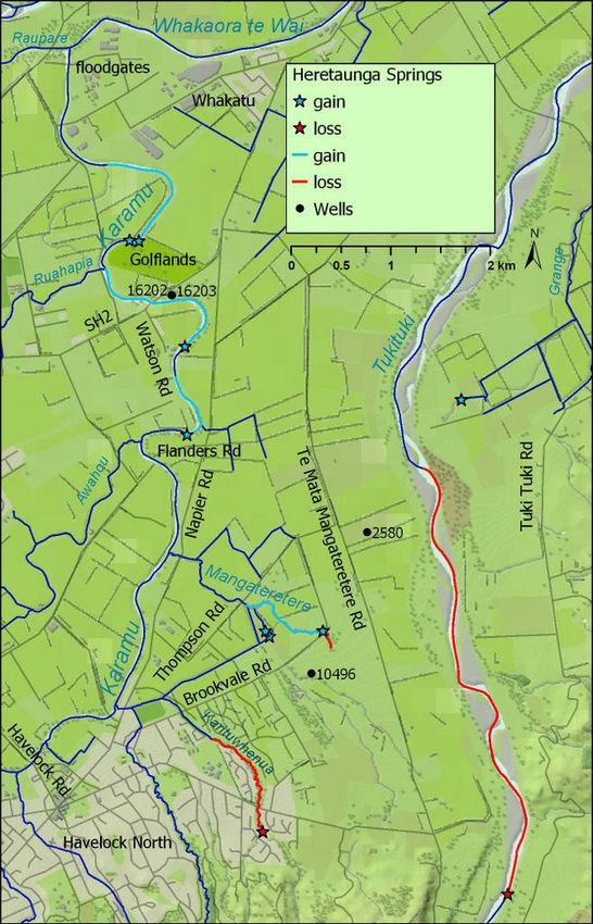
the edge of this confining layer, as well as from holes and fractures close to the edge. Those holes can take
the form of gravel and sand interspersed through the confining layer, creating a semi-confined aquifer
(Harper & Hughes, 2009). Inland of the confining layers, the uncapped gravels can receive recharge water
from the Ngaruroro, Tukituki and Tutaekuri rivers (detailed in this report), in addition to direct rainfall
recharge.
The formation of hard pans can inhibit the movement of rainfall recharge down through the soil profile. Three
types of pan could be present on the Heretaunga Plains:
pan cemented by lime (calcium carbonate) that is weathered from adjacent limestone hill-country;
wind-blown silt (loess);
duripan with silica from Taupo airfall ash (Griffiths, 2001).
In addition to the airborne ash, the Ngaruroro River delivered a large load of alluvial pumice from more recent
Taupo eruptions (e.g. 177 AD). This formed a shallow deposit of pumice sand over extensive areas of the
Heretaunga Plains (Grant, 1996; Griffiths, 2001), providing a conduit for shallow groundwater. Another
conduit for shallow groundwater is provided by river gravels deposited on top of the confining layer by more
recent flowpaths. For example, Rabbitte (2011) proposed that flow losses from the Ngaruroro River could be
conveyed to adjacent springs via shallow sand or gravel above the confining layer. Where hard pans are
lacking from the soil, these conduits for shallow groundwater are open to rainfall recharge and nutrient
leachate.
Earthquakes are also an important physical driver, buckling the hill country around the plains, and fracturing
the rock in a way that controls groundwater flow (Cameron et al., 2011). Earthquakes have also tilted the
Heretaunga Plains themselves (Lee et al., 2014). The 1931 earthquake lifted large areas sufficient to change
the flowpath of some streams, and new springs have emerged after smaller earthquakes (e.g. via fracturing
of the confining layer).The complexity of these interacting physical drivers creates a diverse array of habitats
both on land and in streams (Hauer et al., 2016; Wakefield et al., 2012).
Heretaunga Springs 9
Figure 1-2: Groundwater beneath the Heretaunga Plains. The movement of groundwater through gravel layers
(blue layers) is contained within confining layers of clay (brown layers). This figure provides a stylised representation
of these elements, rather than a geological map. Artwork by Chris Davidson, 4art.co.nz.

1.4      Climate
The Heretaunga Plains have a maritime-temperate climate, with approximately 800 mm of rainfall and 2150
sunshine hours each year (Chappell, 2013). The seasonality of rainfall is small compared to the high
evaporation rates through summer, which increase water demand for irrigation. The ranges west of the
Heretaunga Plains (e.g. Ruahine, Kaweka) capture high rainfall from westerly weather systems. The colder
and wetter climates in the ranges generate higher flows in the mainstem rivers (Ngaruroro, Tukituki,
Tutaekuri), compared to lowland areas, and this contrast is more pronounced through summer and autumn.

The low rainfall increases the dependence of horticulture on irrigation. Most irrigation water for the
Heretaunga Plains is sourced from groundwater (HBRC, 2014). Intensive development of the Heretaunga
gravel aquifers provides irrigation water for orchards, vineyards and crops, alongside town and industrial
water supplies.

10                                                                                               Heretaunga Springs
2       Methods
2.1     Locating Springs and Measuring Flow Gains
Aerial photographs were used as a first step to narrow down where each stream started flowing. Talking to
landowners was often the next step. People who have lived on the land often have the best local knowledge
of springs in the area and their history. Having narrowed down the areas of interest, walking the length of
headwater streams provided valuable information on the location of springs, and the start point for the
stream network (Wilding, 2016). The location of each spring (NZTM easting and northing) was recorded from
a handheld GPS (e.g. Garmin GPSMap64, Garmin eTrex).

The location of a spring will change little over time if it is a point spring that arises through a hole in a confining
layer. However, the start location of a diffuse headwater spring will change, with spring flow arising further
upstream during the wetter months when groundwater levels are higher. The timing of spring surveys is
therefore important. This study targeted dry conditions (e.g. the 2013 drought) for spring surveys because
the focus was on perennial streams and their flow requirements (Wilding, 2016).

Only high-priority streams were surveyed on foot. This included streams where flow was spring-dominated;
where groundwater was probably fed from outside the surface water catchment, and springs that
contributed a large proportion of flow to the Heretaunga streams (Paritua-Karewarewa, Irongate,
Mangateretere, Karamu, Tutaekuri-Waimate, Raupare). For other streams, spring mapping relied more
heavily on aerial photographs. A time-series of aerial photographs was available from Google Earth. These
provided visible indicators, including ponded water in adjacent paddocks during dry periods, more wetland
vegetation (e.g. riparian willows, Batelaan et al., 2003), and intensified drainage of adjacent paddocks. A
change in soil classification (Griffiths, 2001) was sometimes observed. Often these indicators can only be
seen from the air, rather than when standing in the stream. Therefore, aerial photographs are
complementary to walking the reach. A time-series of images from Google Street View could distinguish dry
from wet channels at road crossings (winter and summer).

Not all spring inputs can be seen with the naked eye. Diffuse spring inputs to flowing streams are not visible,
and even the large, discrete springs can be masked within large rivers. Therefore, measurements are needed
to detect the start or end of spring inflows in the flowing part of the stream, and these methods are described
in Sections 2.1.1 to 2.1.5.

2.1.1 Direct Flow Measurement (Gauging methods)
The flow measurements that were used in the estimation of flow gains and losses span more than 60 years.
Mechanical flow meters were mostly replaced with acoustic Doppler velocity sensors in the late 2000s. Most
flow measurements undertaken specifically for this study used the Sontek Flowtracker mounted on a wading
rod. Velocity and depths were typically sampled from at least 20 offsets/locations across the channel.
Velocity was sampled for a period of 40 seconds at each offset, and typically sampled at 60% of depth to
approximate mean water column velocity. Site selection and gauging methods otherwise followed guidance
from the National Environmental Monitoring Standards in pursuit of a “fair” quality code (i.e. QC 500),
(Willsman et al., 2013). The data were checked then stored on Hawke’s Bay Regional Councils hydrometric
database (Hilltop Manager).

Other methods were used as and when required. For example, when the stream was not wadable, a boat
mounted acoustic Doppler current profiler (ADCP) was used to measure flow (Sontek M9). Between 4 and 8
passes were typically made, and the flow estimates from replicate passes were averaged to provide a flow
estimate in pursuit of a “fair” quality code (Willsman et al., 2013).

Heretaunga Springs                                                                                           11
Conventionally, spring inflows are detected by gauging the flow at points along the stream, then determining
if there is a change in flow that cannot be explained by tributary inflows. However, relying on stream gauging
imposes limitations on the spatial resolution of the survey, as the number of points along a stream where
flow can be accurately measured is limited, and the smaller the flow change that we seek to detect the more
accurate those measurements need to be. For instance, in braided rivers, several kilometres can separate
suitable gauging locations (i.e. uniform straight runs). For weedy streams, suitable gauging locations may
only exist at road crossings (e.g. culvert outlets), where the distortion of the velocity profile by weed beds is
minimised. This distance between sites will limit our ability to resolve where springs start and end. Other
methods were therefore used to enhance and extend the detection of spring inflows, including the change
in electrical conductance and the change in water temperature from spring inflows.
Flow measurements for this study were generally conducted during periods of steady flow. Periods of rainfall
produce rapid changes in flow that reduce comparability with other sites gauged on the same day. A lot of
the flow data used in this report was not collected specifically for this study. Unless noted otherwise, these
flow data were filtered to remove periods of rapid flow change. Flow was considered rapidly changing if the
difference between daily maximum and daily minimum flow was more than 30% of minimum flow for the
previous 3 days.
2.1.2 Longitudinal Electrical Conductance
The inflow of spring water can be estimated using the downstream change in electrical conductance, if the
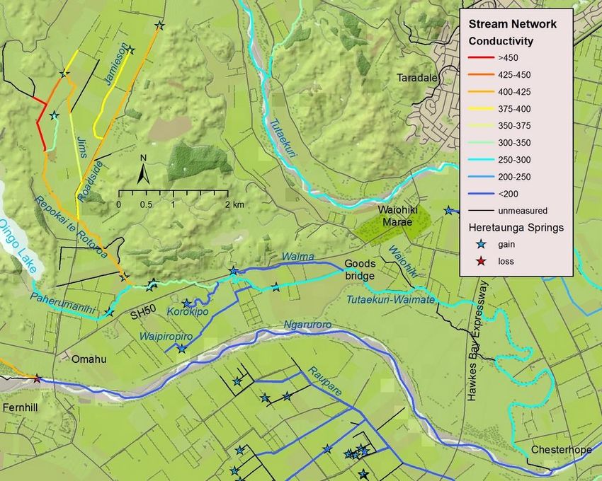
spring water has a different conductance to the river flow. This situation arises in the Karamu Stream and
Tutaekuri-Waimate Stream. These streams are also large enough to be kayaked, with electrical conductivity
sensors (standardised to specific conductance at 25°C) mounted on the kayak, together with synchronised
GPS tracking to provide a location for each measurement. If combined with flow gaugings at the start and
end of the study reach, the downstream change in conductance can then be converted to a flow-profile using
Equation 2-1.
Equation 2-1: Estimating flow gain from electrical conductance. Flow at stream location i is estimated using the
change in EC (Electrical Conductance, µS/cm at 25 °C) between location i and the previous location (i-1), calculated as
a mass flow (EC x Flow L/s). This also requires an estimate of electrical conductance for the spring inflow (ECspring) from
Equation 2-2.
Flowi Flowi 1 Flowi 1 ECi 1 Flowi 1 ECi ECi EC spring
The average conductance of the spring inflow was estimated for each survey, using same-day gaugings
upstream and downstream of the gaining section (Equation 2-2). This assumed the conductance of spring
water did not change significantly over the gaining reach. For example, if spring conductance was actually
lower in downstream reaches, then the relative contribution of downstream springs would be over-
estimated. The measured length of gaining sections likely extended beyond the actual spring inputs because
of the added distance needed to achieve complete mixing (both vertically and horizontally).
Equation 2-2: Estimating spring electrical conductance. The average EC (Electrical Conductance, µS/cm at 25 °C) of
inflowing spring water was estimated using this mass balance equation, using flow (L/s) and electrical conductance
measurements downstream (Flowdown and ECdown, respectively) and upstream (Flowup and ECup, respectively) of the
gaining reach.
EC spring Flowdown EC down Flowup ECup Flowdown Flowup
12 Heretaunga SpringsThe distance between each measurement was estimated from the metric GPS data (NZTM) (Equation 2-3). This was then converted to a distance downstream of the starting point by accumulating the distances between measuring points. The close spacing of measurements (typically
too deep to wade and has too much aquatic plant growth for a boat-mounted flow-meter (ADCP). Only two
suitable locations, with less plants and a more stable bed (exposed cobble at Watson Rd; coarse sand at
Flanders Rd), were identified during the kayak survey. Considerable time was still required to clear weed, and
the deeper areas were marginal for wading, even under low-flow conditions. A good flow estimate was
obtained at Flanders Rd, with four passes by the M9 ADCP (mounted on the hydroboard) providing flow
estimates within 5% of the mean. The flow measurements at Watson Rd were more variable (within 22% of
mean, from 8 passes).

A third kayak conductance survey was completed 5/2/2015 between Flanders Road and the Raupare
confluence (Hach HQ40d, Garmin GPSMap60). The Karamu was gauged the day before, both at floodgates
and at Havelock Road. Flow from rated stage was used to estimate inflow from the Mangateretere Stream.
Data from a fourth run at higher flows (10/11/2016) could not be used because the GPS memory card filled
up (1 second readings generated too much data) and because a large unaccounted flow was entering the
Karamu via the Karituwhenua Stream (Brookvale municipal well testing).

A similar longitudinal conductance survey was completed for the Tutaekuri-Waimate Stream. Conductance
was surveyed between Swamp Rd and the Goods Bridge monitoring site (6.2 km, Figure 3-35), and this was
intended to delineate gains downstream of the reach surveyed by GNS using Distributed Temperature
Sensing (Moridnejad, 2015). The electrical conductance survey was completed on 4/12/2015, with a sampling
interval of 10 seconds for conductance and temperature (Hach HQ40d) and every 5 seconds for GPS location
(Garmin GPSMap64, with GPS & GLONASS receiver). The conductance clock was 2 seconds faster than the
GPS clock, and this offset was removed in post-processing. The conductance sensor was calibrated against a
1413 µS/cm standard on 2/12/2015, and was checked against the same standard after the survey (measured
1430 in the 1413 µS/cm standard, after 1 hour for temperature stabilisation). Flow gaugings were completed
2 days prior to the kayak survey on 2/12/2015 both upstream (Roadside Drain plus Repokai te Rotoroa) and
downstream (Goods Bridge) of the survey reach. Stage monitoring at Goods Bridge confirmed negligible flow
change between flow and conductance measurements (0.1% change in rated flow). The flow magnitude from
each tributary through the survey reach was calculated from dilution of their measured conductance
(Paherumanihi, Korokipo, Waipiropiro, Waima).

2.1.3 Spot Conductance
The use of electrical conductance is not limited to intensive studies. It can also be used as a screening tool,
before committing to more intensive investigations. Spot measurements of electrical conductance at easily
accessible locations (or archived data) can quickly identify large changes in chemistry. For example, a single
visit to Waitio Stream revealed a large drop in conductance between the hill country and Ohiti. This was then
used to define the section of stream targeted for closely spaced measurements of conductance and flow.
Prior to this investigation commencing, spot measurements of electrical conductivity were used to
investigate spring inputs to the Tutaekuri-Waimate Stream (Rabbitte, 2011).

The electrical conductance method will only reveal spring inflows if there is sufficient contrast in conductance
between the stream inflows and the groundwater springs. The greater the spring input (as a proportion of
stream flow), the smaller the contrast in conductance required to detect the spring input.

2.1.4 Longitudinal Temperature
Groundwater temperatures are typically stable (e.g. 15 ± 0.5 °C across seasons), compared to stream
temperatures that can increase 10 °C from night to day. This provides an opportunity for detecting spring
inflows using temperature, in much the same way as electrical conductance. Compared to using electrical
conductance, the benefit of using temperature is that it does not depend on different sources feeding the
stream and groundwater (e.g. to achieve a contrast in major ions). However, the difficulty with using

14                                                                                      Heretaunga Springs
temperature is that stream water temperature increases through the day, and along the length of the stream,
making interpretation of temperature changes between spot measurements difficult. GNS (Institute for
Geological and Nuclear Sciences) overcame this problem by using a 1 km long fibre optic cable that was laid
on the bed of the river. This measures temperature at hundreds of points along its length at the same time,
and repeats all these measurements day and night to capture the largest temperature contrast. This
specialised DTS (distributed temperature sensing) equipment was deployed by GNS in the Tutaekuri-
Waimate to quantify flow gains upstream of State Highway 50. See the GNS reports for more detailed
methods (Moridnejad, 2015). Deployments were also made by GNS in the Ngaruroro River, though the results
are not yet available.
2.1.5 Stable Isotopes of Water
The origins of groundwater, and the springs fed by groundwater, are concealed from view. In large alluvial-
valleys, like the Heretaunga Plains, flowpaths can cross surface catchment boundaries via underground gravel
channels deposited by prehistoric rivers (i.e. palaeochannels). Measuring the isotope ratios of a given spring
can offer clues to where the water has come from, especially if each potential source has a unique isotope
ratio (Taylor et al., 1989).
Stable isotopes of water are naturally occurring, do not degrade in groundwater, and are inexpensive to
sample and analyse (Stewart & Taylor, 1981). These isotopes are useful for spring investigations because
each river can have a unique isotope ratio (or isotopic signature). For example, a river draining cool mountain
ranges will have more negative values of δ18O and δ2H, compared to a stream draining warm lowland areas
(Stewart & Taylor, 1981).
The heavy water isotopes are less likely to evaporate from the ocean, and more likely to fall as rain. Cold
temperatures affect the isotopes’ movement from ocean, to clouds, to rain - more so than normal water. The
net effect of this discriminatory movement is measured using δ18O and δ2H, with ocean water producing
values close to zero, compared to rain that produces more negative values. Rainfall in colder areas, and areas
further inland, produce more negative values again. For a more detailed description of these physical
processes, and other applications for isotope tracers, see Stewart and Morgenstern (2001). The heavy
isotopes of water were used as tracers for this report, including:
δ18O – the isotope ratio of heavy oxygen 18O to normal oxygen 16O, divided by the standard isotope
ratio for seawater (Vienna Standard Mean Ocean Water). Units are ‰ (parts per thousand).
δ2H – the isotope ratio of heavy hydrogen 2H (deuterium) to normal hydrogen 1H, divided by the
standard isotope ratio for seawater (Vienna Standard Mean Ocean Water). Units are ‰.
Isotope sampling for this spring investigation was an add-on to water tracing and aging investigations
initiated for groundwater modelling of the Heretaunga Plains (Morgenstern et al., 2018). Some additional
springs, streams and wells were sampled for this report, focussing on the spring inflows to the Karamu and
Mangateretere streams whose origin was in question. Most warm-season sampling was conducted 3 and 4
March 2015 (Appendix B), when river levels were extremely low (e.g. flow for Ngaruroro at Fernhill was less
than half the mean annual low flow). This sampling run covered the Karamu Stream, Mangateretere Stream,
and the potential recharge rivers (see Appendix B for sites and results). Sampling of some additional springs
and shallow wells (well number 2580 and 16202) was conducted 6 and 12 March 2016, again under extreme
low-flow conditions. A second round of sampling for stable isotopes was completed in winter to help
understand seasonal changes in groundwater origin. This was completed 23/8/2017, targeting winter
baseflow conditions. A subset of sites was chosen to represent the lower Karamu Stream and upper
Tutaekuri-Waimate. Additional sites were sampled to represent potential source water (Appendix B).
Heretaunga Springs 15The stable isotopes reported here did not require special sample handling. Wells were purged to flush stagnant water from the casing, using casing volume and pumping rate to estimate the pumping time required. Electrical conductance was also monitored using a hand held probe to confirm the purged water had reached static levels before sampling. Samples were collected in bottles supplied by the GNS Stable Isotope Laboratory, who analysed the samples using isotope ratio mass spectrometry with reported precisions of 0.1 ‰ for δ18O and 1.0 ‰ for δ2H (Morgenstern et al., 2018). Chemistry samples were collected at the same time, and sent to Hill Laboratories for analysis of major ions and nutrients. For rivers and streams, flow measurements were made within 24 hours of sampling, under prevailing stable- flow conditions (see Section 2.1.1 for gauging methods). The two exceptions were warm-season sampling of the Mangateretere Stream and Tukituki River, for which flow was calculated from rated water level, which is not as accurate as gauged flow. Where isotope samples were collected directly from the spring head, flow was not measured. Rain falling directly onto the Heretaunga Plains is a potential source of the groundwater that feeds springs, in addition to the river recharge sources described in the results (Sections 3.1, 3.2 and 3.3). The isotope signature of local rainfall was not sampled for this study because the high variability of heavy-water isotopes in rainfall (between seasons and rainfall events) necessitates long-term monitoring to adequately characterise this source (Stewart & Taylor, 1981). Data were obtained from GNS (Baisden et al., 2016) for two locations at low-elevations close to the Heretaunga Plains (station 29509, Lat. -39.425 Long. 176.825, n=33, station 30050 Lat. -39.725 Long. 176.975, n=30). These were sampled monthly between 2007 and 2010, revealing the more negative δ18O from winter rainfall compared to summer (Figure 2-1). Bias towards months that were sampled more often over the three year period was removed by first averaging all January samples across years, and so on for other months, before averaging over the 12 calendar months. The long- term mean δ18O was -5.9‰ (δ2H -36.0‰) for site 30050. The mean δ18O was more negative for the other site (station 29509), with δ18O of -6.7‰ (δ2H -42.4‰). However, an outlier in April (Figure 2-1) had high leverage on this mean (excluding outlier δ18O -6.3‰, δ2H -39.5‰). An estimate for rainfall for the unconfined recharge area of the Heretaunga Aquifer was calculated using the isoscape model developed by Baisden et al. (2016). This predicted a long-term mean δ18O of -5.0‰ (δ2H -36.0‰) for the selected Virtual Climate Station (station 28640, Lat. -39.625, Long. 176.775, elevation 19 m, period July 2013 to June 2015). 16 Heretaunga Springs
Figure 2-1: Stable isotopes in rainfall by month. The δ18O for rainfall samples collected at two sites (30050 and
29509) close to the Heretaunga Plains. Samples were collected for a separate study (Baisden et al., 2016) between
2007 and 2010, and are over-plotted by calendar month.

Understanding the isotopic signature of rainwater is the first step in understanding the isotopic signature of
groundwater originating from local rainfall recharge (Gat, 1995; Stewart & Taylor, 1981). Small rain events
falling on dry soils can evaporate or run off before reaching groundwater, producing a seasonal bias to
recharge in winter and spring. But, in addition to seasonal bias, the water that is recharged has been
fractionated by evaporation of lighter isotopes from plant and soil surfaces (Gat, 1995). Hence, the bias
toward more negative δ18O from winter recharge is countered by a bias to less negative δ18O as a
consequence of evaporative fractionation (Gat, 1995). In the absence of lysimeter isotope data, an
appreciation of the net effect of these, and other, physical processes on the isotopic signature of rainfall
recharge (i.e. the isotopic transfer function) is provided by streams draining low-elevation sub-catchments,
particularly those lacking inter-basin groundwater connections and lakes. The least negative isotope
signatures were observed in such catchments, with δ18O in the range of -5.8‰ to -6.0‰ and δ2H of -35‰ to
-38‰ (e.g. Paritua at water wheel 4/3/2015, Kaikora upstream of Papanui confluence 17/4/2015,
synthesized Awanui upstream of Karewarewa 3/3/2015). Not all low-elevation catchments were this high.
For example, the stream draining the highest elevation sub-catchment had a δ18O of -6.8‰ and δ2H of -41‰
on 5/3/2015 (Te Waikaha Stream at Mutiny Road drains Mt Erin). In the absence of direct measurements
from lysimeters, this report used interim δ18O of -6.0‰ and δ2H of -39‰ to characterise rainfall recharge on
the Heretaunga Plains (average Awanui, Karewarewa, Paritua and Kaikora streams during low flow
conditions).

Heretaunga Springs                                                                                         17
2.2     Measuring Flow Losses
The physical processes by which spring inflows from groundwater enter streams are the same, in many
respects, to flow losses from streams to groundwater. The change from a gain to a loss occurs when the
groundwater level drops below the stream level. However, there are fewer options for measuring a loss of
flow from a stream, compared to measuring a gain. For example, the downstream change in electrical
conductance cannot be used to measure a flow loss because the concentration of major ions is not affected
by a flow loss (i.e. major ions are lost along with the flow). For this investigation, measuring a flow loss
required direct measurement of the stream flow at discrete locations along the river (the change in flow
equating to the net loss). As described in Section 2.1, the number of points along a stream where flow can
be accurately measured is limited. This distance between suitable sites will limit our ability to resolve where
losses start and end.

In some cases, it was possible to refine the end of a losing section using an estimate of groundwater level
(i.e. where stream level was the same as the adjacent groundwater level). Indicators of adjacent groundwater
level include recorded water level from nearby wells, or the elevation of adjacent springs. These do not give
an exact representation of the groundwater level directly below the riverbed. However, this information can
improve the delineation compared to gaugings spaced several kilometres apart. Other evidence that was
useful for locating springs (e.g. wetland vegetation), were sometimes also useful in narrowing down the end
of a losing reach (see Section 2.1).

3       Results
In total, 64 spring locations were mapped for this report (Appendix A). These are described separately for
each sub-catchment.

3.1     Ngaruroro
Flow losses to groundwater
The lower Ngaruroro River typically loses more than 4000 L/s to groundwater. This recharges the Heretaunga
aquifer which, in turn, feeds many of the springs on the Heretaunga Plains. The Ngaruroro is the most
intensively gauged river on the Heretaunga Plains (Dravid & Brown, 1997; Grant, 1965), with flow losses
measured from 336 concurrent gaugings dating back to 1952. This is in addition to the 1392 gaugings at
monitoring sites on the Ngaruroro River (Whanawhana, Fernhill and Chesterhope). Flow gaugings are the
only way to measure flow losses at present (Section 2.2), because the loss of water has little effect on the
chemical characteristics of the water (compared to spring inputs).

Most of the flow loss from the Ngaruroro occurs between Roys Hill and Fernhill (Dravid & Brown, 1997; Grant,
1965), with a median loss of 4250 L/s (107 concurrent gaugings at median gauged flow of 7020 L/s at Fernhill).
This 5 km length of river is termed the “major loss” reach (Figure 3-4). The material underlying this reach
includes unconfined gravels (see Section 1.3). The concurrent gaugings demonstrate some variability in the
amount of water lost from the river (interquartile range 3900 to 4600 L/s loss). Some of this variability is
attributable to measurement error, and the L/s of measurement error increases with flow (e.g. 10% error
equates to ±100 L/s error at 1,000 L/s river flow, or ±10,000 L/s error at 100,000 L/s river flow). In addition,
the true loss from the river can change over time. When groundwater levels are lower, more water may be
lost from the Ngaruroro River (Dravid & Brown, 1997). Higher river flows can also increase the amount of
flow lost, by increasing the pressure head and the area of wetted gravel through the losing reaches. However,
there was a lack of correlation between flow loss and the total river flow, or groundwater level (R2 = 0.02 and

18                                                                                      Heretaunga Springs
0.01 respectively). Likewise, lower groundwater levels did not increase the likelihood of more loss (odds ratio
0.8 for flow loss >4250 L/s at groundwater levels
Figure 3-1: Ngaruroro flow-loss downstream of Fernhill. The magnitude of flow loss was variable and, when there
was a loss, it typically occurred within 3 km downstream of Fernhill. To demonstrate this, Fernhill flow was subtracted
from each gauging on the same day. Therefore, Fernhill is plotted as zero flow change, and negative values represent
a flow loss. Each site is represented on the x-axis by its distance downstream of Fernhill, so Fernhill Bridge is at 0 km
and Chesterhope Bridge is at 10.7 km. These dates were selected for this plot because multiple sites were gauged
downstream of Fernhill (excluded gauging dates covered fewer sites). The flow increase at 10.7 km (Chesterhope)
reflects the inflow from the Tutaekuri-Waimate Stream (see map, Figure 3-4).

An additional “minor loss” reach may also occur upstream of the major-loss reach (Figure 3-4). Dravid and
Brown (1997) estimated the minor loss at 800 L/s. A similar magnitude of loss was estimated for this report,
using different methods. The inflows located upstream of Ohiti were measured, including from the mainstem
(Ngaruroro at Whanawhana), in addition to tributaries between Whanawhana and Ohiti (Poporangi,
Otamauri, Mangatahi, Kikowhero, Maraekakaho, Figure 3-4). Using eight concurrent gaugings that included
sites on all tributaries, the median loss was 450 L/s (interquartile range 350 to 750 L/s), (Figure 3-2). The
actual loss would be higher if there were additional seepages from valleys draining directly to the river
mainstem. Conversely, the actual loss would be lower if some of the flow that is lost subsequently returns to
the Ngaruroro downstream of Ohiti (e.g. via Waitio Stream).

The location of this minor loss is uncertain. For example, Dravid and Brown (1997) defined the minor loss
zone as the reach between Maraekakaho to Roys Hill (Figure 3-4), despite using concurrent gaugings from
more than 10 km further upstream (Mangatahi) in estimating the magnitude of loss. The small number of

20                                                                                              Heretaunga Springs
concurrent gaugings between Whanawhana and Ohiti, together with the small proportion of flow that is lost
or gained, prevents better spatial definition of where the gains and losses occur.

Another outstanding issue is the potentially large subsurface flow proposed by Grant (1965). It is reasonable
to expect some water to travel as groundwater through the alluvial gravels, in addition to the surface flow.
But the magnitude of subsurface flow proposed by Grant (1965) is surprisingly high (30% of flow). Grant
(1965) observed that the flows for the Ngaruroro at Mangatahi exceeded the sum of inflows, and concluded
that additional flow was missed at upstream sites (e.g. Whanawhana) because it travelled as subsurface flow.
It is unclear why this subsurface flow would resurface at Mangatahi, given this sites alluvial valley setting,
compared to Whanawhana, which is confined within a bedrock canyon. A closer look at the concurrent
gaugings indicates that the higher flows observed at Mangatahi might be attributable to gauging error. Grant
(1965) based his conclusions on two concurrent gaugings (28/11/1961 and 13/2/1964). Subsequent gaugings
instead indicate that, at most sites on most occasions, the measured Ngaruroro flow is equivalent to, or less
than, the summed inflows (Ngaruroro at Whanawhana plus gauged tributaries). Of 73 gaugings along the
Ngaruroro, 68 measurements were equivalent to, or less than, the estimated sum of inflows, allowing for a
10% margin of gauging error (Figure 3-3). It is possible that those five (out of 73) gaugings with higher than
expected flows reveal a large sub-surface flow. However, it is a weak evidence in its own right.

Figure 3-2: Ngaruroro flow losses upstream of Ohiti. The flow measured at Ohiti is plotted against the flow
expected if there were no losses, which was estimated from gaugings at Whanawhana, plus all major tributaries
(Poporangi at Ohara Station, Otamauri at Whanawhana Rd, Mangatahi at Aorangi Rd, Kikowhero at Crownthorpe Rd,
Maraekakaho downstream of Tait Rd). Each point is a concurrent gauging run, with all major tributaries gauged on
eight occasions (28/11/1961, 13/2/1964, 11/11/2009, 16/12/2009, 20/1/2010, 24/3/2010, 14/4/2010, 28/4/2010,
5/3/2013). A linear trend line is fitted to all eight dates (solid line, with equation). Points below the dotted-line (1:1)
indicate a net flow loss to groundwater.

Heretaunga Springs                                                                                                 21
Figure 3-3: Ngaruroro measured flow versus summed inflows. Flows for Ngaruroro at Mangatahi (red dots)
exceeded the sum of inflows (x-axis) on several occasions (red points above solid line), leading Grant (1965) to
conclude that large subsurface flows were reappearing at this site. The alternative explanation is that the higher flows
recorded at Mangatahi were attributable to measurement error. To investigate the alternative, this plot demonstrates
the small number of flow measurements that exceeded summed inflows by more than a 10% margin of error. The
inflows were gauged on 8 occasions, and inflows for other occasions were estimated from correlations of tributary
inflows with Whanawhana. Points above the solid black line had measured flow that exceeded the sum of inflows. The
dotted-lines delineate a nominal 10% margin of measurement error (QC500, Willsman et al., 2013).

22                                                                                             Heretaunga Springs
413
                                                                                                                                          Puketapu
                                                                                                                                                                 Napier

              Whanawhana

                                                                                                                                                               Brookfields Bridge
                                                                                                                          Fernhill
                                         Mangatahi
                                                                                                                               Variable
                                                                                                 Ohiti
                                                                                                                                 loss
                                                                                                                                                     Chesterhope
                                                                                                                                                        Bridge

                                                                                                                                                                  Karamu Stream
                                                                                                           Roys Hill

                                                                         Maraekakaho
                                                                                                                                                 Hastings

Figure 3-4: Ngaruroro River. Map of the Ngaruroro River showing the location of flow monitoring sites (e.g. Whanawhana, Fernhill and Chesterhope Bridge), reaches
that lose flow to groundwater (Major loss and Variable loss) and the fish-habitat survey reach (Johnson, 2011a). The location of the “Minor loss” reach upstream of Roys
Hill is uncertain (see text). The section of river that was diverted to a constructed channel is also labelled (“diversion”), in addition to the approximate Ngaruroro
flowpath prior to the 1867 flood. Selected monitoring wells (black dots) are labelled with the well number.

Heretaunga Springs                                                                                           23
Stable isotopes of water The major loss of flow from the Ngaruroro River to the Heretaunga aquifer makes it a likely source for many of the groundwater springs in neighbouring catchments. Stable isotopes can be used to trace groundwater originating from the Ngaruroro, provided it has an isotope signature that is distinct from other sources (Section 2.1.5). For example, Taylor noted more negative values of δ18O for Ngaruroro water (Section 7.8 in (Dravid & Brown, 1997). Stable isotope ratios for river water can vary seasonally, and in response to rainfall (Stewart & Taylor, 1981). Wells that are located close to the river recharge source typically provide a less variable isotope ratios that better typify the groundwater originating from that recharge source, compared to a single river sample (Scott, 2014). To determine the isotope signature of Ngaruroro sourced groundwater, samples of groundwater were collected from a shallow well closer to the Ngaruroro major loss reach (well no. 10340, 17 m deep, 2.5 km from river, Figure 3-4). This groundwater had a mean δ18O value of -7.6‰ (-7.5‰ on 23/6/2014 and -7.7‰ on 23/8/2017). Groundwater wells with a δ18O value of -7.5‰ to -7.7‰ were widespread across the Heretaunga Plains (e.g. -7.6‰ from well 1459 at 53 m, -7.6‰ from well 15003 at 55 m, -7.7‰ from well 16361 at 23 m). However, other wells that are also likely to be sourced from the Ngaruroro had more negative δ18O between -7.8‰ and -8.2‰, and these occurred at a range of depths (e.g. -7.8‰ from well 16360 at 65 m, -8.0‰ from well 5915 at 38 m, -8.2‰ from well 1674 at 38 m). Results from the river itself help shed light on some this variability (Figure 3-5). Samples collected for this study ranged from -7.4‰ in March (mean of two sites sampled 3/3/2015) to -8.1‰ in August (mean of four sites sampled 23/8/2017). Previous monitoring of isotopes from the Ngaruroro River (Morgenstern et al., 2018) produced a wider range of δ18O values (Figure 3-5). To maximise the generality of sampling to date, the relationship between δ18O and ocean temperature was used to predict mean δ18O for a longer period of time (Figure 3-5). This relationship was based on the mean sea-surface temperature for the Tasman Sea for the month prior to isotope sampling (www.bom.gov.au/cgi-bin, data accessed 31/10/2017). In addition to affecting evaporation from the sea surface, the temperature of the ocean also affects the weather patterns that drive local rainfall and evaporation. These predictions from ocean temperature demonstrate the inter- year climate variability that contribute to the spatial variability of δ18O in groundwater (Figure 3-6). For example, well 413 in Napier (Figure 3-4) was estimated to have a mean residence time of 110 years (Morgenstern et al., 2018). The more negative δ18O of -8.08‰ for this well corresponds with more negative river δ18O of -8.16‰ predicted for 110 years prior to sampling. The climate was generally cooler then, and hence river water from recent years is predicted to have a less negative δ18O of -7.9‰ (-7.90‰ for 2013- 2017, -7.92‰ for 2008-2017, -7.93‰ for 1998-2017). Heretaunga Springs 24
Figure 3-5: Oxygen stable isotopes in river water. The data for stable isotopes of oxygen (δ18O) from Morgenstern
et al. (2018) for the period 2009-2010 (Ngaruroro at Chesterhope, Tukituki at Red Bridge) are plotted together with
samples collected for this study in March 2015 and August 2017 (Ngaruroro, Tutaekuri and Tukituki). Over-plotting the
datasets by calendar month demonstrates both the seasonal and the inter-annual variability in δ18O. This also
demonstrates the consistent pairwise difference between the Ngaruroro and Tukituki rivers (paired t-test P
Figure 3-6: Predicting long-term δ18O using sea surface temperature. The upper plot shows the relationship
between river samples of δ18O (Tukituki and Ngaruroro) and mean surface temperate of the Tasman Sea for the
month prior to each sample. This excludes two sample dates when flow fluctuations were high (July 2010, October
2010). Using the equation from the upper plot, δ18O was predicted for other years for which we have sea-surface
temperature (annual mean for the water year).

26                                                                                         Heretaunga Springs
Adopting a δ18O signature of -7.9‰ for Ngaruroro River water still leaves a shortfall in explaining the many
wells with δ18O closer to -7.6‰. Morgenstern et al. (2018) concluded that these wells with a less negative
δ18O were influenced by local rainfall recharge, going so far as to suggest a δ18O of -7.6‰ may represent the
isotope signature of rainfall recharge. In the absence of lysimeter samples, or similar, to characterise rainfall
recharge on the Heretaunga Plains, this report adopted an interim δ18O of -6.0‰ (Section 2.1.5). This rainfall
signature provides a strong contrast with the value of -7.6‰ seen in many wells, suggesting rainfall made a
minor contribution to groundwater recharge. For example, if local rainwater recharge has a mean δ18O
of -6.0‰ (see Section 2.1.5) and Ngaruroro sourced groundwater had a mean δ18O of -7.9‰, then a mix of
river water with 15% rainfall recharge would be required to produce a mean δ18O of -7.6‰, as observed in
many wells. Seasonal bias in the transfer of river water to groundwater is minimised by the low variability for
the major-loss reach (interquartile range 3900 to 4600 L/s loss).

The contrast between the Tukituki and Ngaruroro river water was sufficient to differentiate the two sources
(Figure 3-5), with a mean difference of -1.1‰ between 17 paired samples (paired sample T-test P
You can also read