A comparison of catchment travel times and storage deduced from deuterium and tritium tracers using StorAge Selection functions

Page created by Clayton Mclaughlin
 
CONTINUE READING
A comparison of catchment travel times and storage deduced from deuterium and tritium tracers using StorAge Selection functions
Hydrol. Earth Syst. Sci., 25, 401–428, 2021
https://doi.org/10.5194/hess-25-401-2021
© Author(s) 2021. This work is distributed under
the Creative Commons Attribution 4.0 License.

A comparison of catchment travel times and storage deduced from
deuterium and tritium tracers using StorAge Selection functions
Nicolas Björn Rodriguez1,2 , Laurent Pfister1 , Erwin Zehe2 , and Julian Klaus1
1 Catchment    and Eco-hydrology Research Group, Environmental Research and Innovation Department,
Luxembourg Institute of Science and Technology, Belvaux, Luxembourg
2 Institute of Water Resources and River Basin Management, Karlsruhe Institute of Technology, Karlsruhe, Germany

Correspondence: Nicolas Björn Rodriguez (nicolas.bjorn.rodriguez@gmail.com)

Received: 25 September 2019 – Discussion started: 14 October 2019
Revised: 23 September 2020 – Accepted: 8 November 2020 – Published: 27 January 2021

Abstract. Catchment travel time distributions (TTDs) are an       5 years. The travel time differences between the tracers were
efficient concept for summarizing the time-varying 3D trans-      small compared to previous studies in other catchments, and
port of water and solutes towards an outlet in a single func-     contrary to prior expectations, we found that these differ-
tion of a water age and for estimating catchment storage by       ences were more pronounced for young water than for old
leveraging information contained in tracer data (e.g., deu-       water. The found differences could be explained by the calcu-
terium 2 H and tritium 3 H). It is argued that the preferential   lation uncertainties and by a limited sampling frequency for
use of the stable isotopes of O and H as tracers, compared to     tritium. We conclude that stable isotopes do not seem to sys-
tritium, has truncated our vision of streamflow TTDs, mean-       tematically underestimate travel times or storage compared
ing that the long tails of the distribution associated with old   to tritium. Using both stable and radioactive isotopes of H
water tend to be neglected. However, the reasons for the          as tracers reduced the travel time and storage calculation un-
truncation of the TTD tails are still obscured by method-         certainties. Tritium and stable isotopes both had the ability
ological and data limitations. In this study, we went be-         to reveal short travel times in streamflow. Using both tracers
yond these limitations and evaluated the differences between      together better exploited the more specific information about
streamflow TTDs calculated using only deuterium (2 H) or          longer travel times that 3 H inherently contains due to its ra-
only tritium (3 H). We also compared mobile catchment stor-       dioactive decay. The two tracers thus had different informa-
age (derived from the TTDs) associated with each tracer.          tion contents overall. Tritium was slightly more informative
For this, we additionally constrained a model that success-       than stable isotopes for travel time analysis, despite a lower
fully simulated high-frequency stream deuterium measure-          number of tracer samples. In the future, it would be useful to
ments with 24 stream tritium measurements over the same           similarly test the consistency of travel time estimates and the
period (2015–2017). We used data from the forested head-          potential differences in travel time information contents be-
water Weierbach catchment (42 ha) in Luxembourg. Time-            tween those tracers in catchments with other characteristics,
varying streamflow TTDs were estimated by consistently us-        or with a considerable fraction of stream water older than
ing both tracers within a framework based on StorAge Se-          5 years, since this could emphasize the role of the radioac-
lection (SAS) functions. We found similar TTDs and sim-           tive decay of tritium in discriminating younger water from
ilar mobile storage between the 2 H- and 3 H-derived esti-        older water.
mates, despite statistically significant differences for cer-
tain measures of TTDs and storage. The streamflow mean
travel time was estimated at 2.90 ± 0.54 years, using 2 H, and
3.12 ± 0.59 years, using 3 H (mean ± 1 SD – standard devia-       1   Introduction
tion). Both tracers consistently suggested that less than 10 %
of the stream water in the Weierbach catchment is older than      Sustainable water resource management is based upon a
                                                                  sound understanding of how much water is stored in catch-

Published by Copernicus Publications on behalf of the European Geosciences Union.
A comparison of catchment travel times and storage deduced from deuterium and tritium tracers using StorAge Selection functions
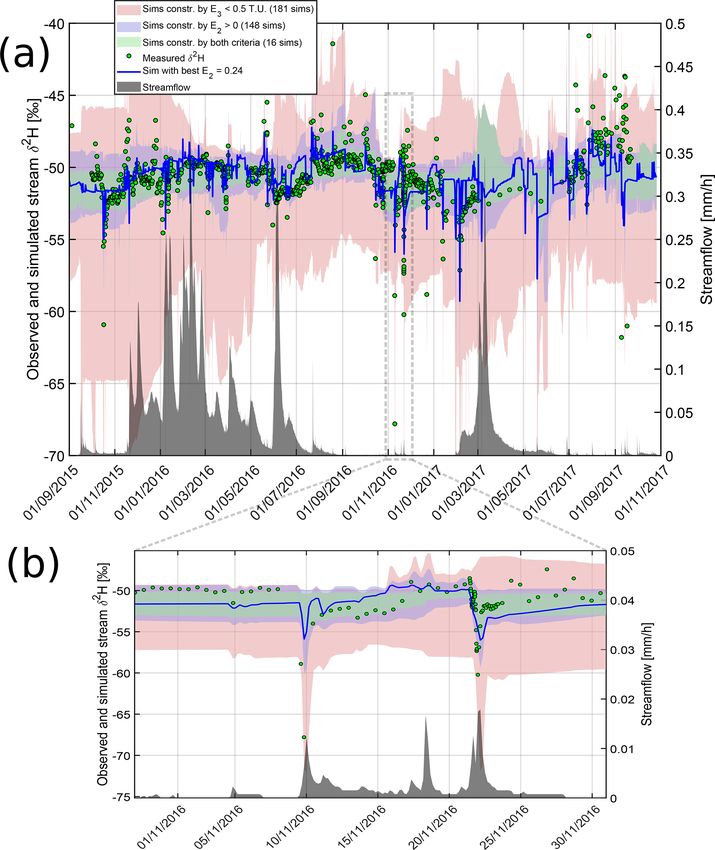
402                                                N. B. Rodriguez et al.: Travel times from deuterium and tritium tracers

ments and how it is released to the streams. Isotopic tracers     ing to Stewart et al. (2012); Stewart and Morgenstern (2016),
such as deuterium (2 H), oxygen 18 (18 O), and tritium (3 H)      the limited use of 3 H may have cause a biased or truncated
have become the cornerstone of several approaches for tack-       vision of stream TTDs in which the long TTD tails remain
ling these two critical questions (Kendall and McDonnell,         mostly undetected by stable isotopes. Longer mean travel
1998). For instance, hydrograph separation, using the sta-        times (MTTs) were inferred from 3 H than from stable iso-
ble isotopes of O and H (Buttle, 1994; Klaus and McDon-           topes in several studies employing both tracers (Stewart et al.,
nell, 2013), has unfolded the difference between catchments       2010). Longer MTTs may have profound consequences for
hydraulic response (i.e., streamflow) and chemical response       catchment storage, which is usually estimated from TTDs as
(e.g., solutes; Kirchner, 2003) related to the different con-     S = Q × MTT (with Q as the flux through the catchment),
cepts of water celerity and water velocity (McDonnell and         assuming steady-state flow conditions (i.e., S(t) = S(t) =
Beven, 2014). Isotopic tracers have also been the backbone        S, Q(t) = Q(t) = Q, MTT(t) = MTT(t) = MTT; McGuire
for unraveling water flow paths in soils (Sprenger et al.,        and McDonnell, 2006; Soulsby et al., 2009; Birkel et al.,
2016) and distinguishing between soil water going back to         2015; Pfister et al., 2017). Under this assumption, a truncated
the atmosphere and flowing to the streams (Brooks et al.,         TTD would result in an underestimated MTT and, thus, an
2010; McDonnell, 2014; McCutcheon et al., 2017; Berry             underestimated catchment storage. A different perspective on
et al., 2018; Dubbert et al., 2019).                              catchment storage and on its relation with travel times may,
   The determination of travel time distributions (TTDs) is       however, be adopted by calculating storage from unsteady
the method that relies the most on isotopic tracers (McGuire      TTDs.
and McDonnell, 2006). TTDs provide a concise summary                 A water molecule that reached an outlet has only one
of water flow paths to an outlet by leveraging the informa-       travel time, which is defined as the duration between entry
tion on storage and release contained in tracer input–output      and exit. The use of different methods of travel time analy-
relationships. TTDs are essential for linking water quantity      sis for stable isotopes of O and H and for 3 H (e.g., ampli-
to water quality (Hrachowitz et al., 2016), for example, by       tudes of seasonal variations vs. radioactive decay) was first
allowing calculations of stream solute dynamics from a hy-        pointed out as a main reason for the discrepancies in MTT
drological model (Rinaldo and Marani, 1987; Maher, 2011;          (Stewart et al., 2012). Further research is thus needed to de-
Benettin et al., 2015a, 2017a). TTDs are commonly calcu-          velop mathematical frameworks that coherently incorporate
lated from isotopic tracers in many subdisciplines of hy-         stable isotopes of O and H and 3 H in travel time calculations.
drology and, thus, have the potential to link the individual      Moreover, several limiting assumptions were used in previ-
studies focused on the various compartments of the critical       ous studies that employed 3 H to derive the MTT, which is
zone (e.g., groundwater and surface water; Sprenger et al.,       in itself an insufficient statistic for describing various aspects
2019). 3 H has been used as an environmental tracer since         (e.g., shape, modes, and percentiles) of the TTDs. For exam-
the late 1950s (Begemann and Libby, 1957; Eriksson, 1958;         ple, the steady-state flow assumption has been used in almost
Dinçer et al., 1970; Hubert et al., 1969; Martinec, 1975), and    all 3 H travel time studies (McGuire and McDonnell, 2006;
it gained particular momentum in the 1980s with its use in        Stewart et al., 2010; Cartwright and Morgenstern, 2016; Du-
diverse TTD models (Małoszewski and Zuber, 1982; Stew-            vert et al., 2016; Gallart et al., 2016). Yet, time variance is
art et al., 2010). It is argued that 3 H contains more informa-   a fundamental characteristic of TTDs (Botter et al., 2011;
tion on travel times than stable isotopes due to its radioac-     Rinaldo et al., 2015), and it has been acknowledged in simu-
tive decay (Stewart et al., 2012). For example, low tritium       lations of stream 3 H only very recently (Visser et al., 2019).
content generally indicates old water in which most of the        Hydrological recharge models or tracer-weighting functions
3 H from nuclear tests has decayed. Despite its potential, 3 H    have also been employed to account for the influence of the
is used only rarely in travel time studies nowadays (Stew-        mixing of precipitation tracer values in the unsaturated zone
art et al., 2010), most likely because high-precision analy-      and for the influence of the seasonal (hence, time-varying)
ses are laborious (Morgenstern and Taylor, 2009) and rather       losses to the atmosphere via ET(t) (e.g., Małoszewski and
expensive. In contrast, the use of stable isotopes in travel      Zuber, 1982) on the catchment inputs in 3 H (Stewart et al.,
time studies has soared in the last 30 years (Kendall and         2007). However, these methods do not explicitly represent
McDonnell, 1998; McGuire and McDonnell, 2006; Fenicia             the influence of the TTD of ET on the age-labeled water
et al., 2010; Heidbuechel et al., 2012; Klaus et al., 2015a;      balance and, thus, represent indirect approximations. In con-
Benettin et al., 2015a; Pfister et al., 2017; Rodriguez et al.,   trast, explicit considerations of ET and of the influence of its
2018). This is notably due to the fast and low-cost analyses      TTD on the streamflow TTD are becoming common for sta-
provided by recent advances in laser spectroscopy (e.g., Lis      ble isotopes (van der Velde et al., 2015; Visser et al., 2019).
et al., 2008; Gupta et al., 2009; Keim et al., 2014) and the      Finally, more guidance on the calibration of the TTD models
associated technological progress in the sampling techniques      against 3 H measurements is needed (see, for example, Gallart
of various water sources (Berman et al., 2009; Koehler and        et al., 2016). The uncertainties of 3 H-inferred travel times, in
Wassenaar, 2011; Herbstritt et al., 2012; Munksgaard et al.,      particular, may have been overlooked, while these could ex-
2011; Pangle et al., 2013; Herbstritt et al., 2019). Accord-

Hydrol. Earth Syst. Sci., 25, 401–428, 2021                                          https://doi.org/10.5194/hess-25-401-2021
A comparison of catchment travel times and storage deduced from deuterium and tritium tracers using StorAge Selection functions
N. B. Rodriguez et al.: Travel times from deuterium and tritium tracers                                                        403

plain the differences in the stable isotope-inferred travel time   (deuterium 2 H) for which we have more precise measure-
estimates.                                                         ments than for oxygen-18 (18 O). A transport model based
   Besides methodological problems, the reasons for the            on TTDs was recently developed and successfully applied to
travel time differences (hence the apparent storage or mix-        simulate a 2-year, high-frequency (subdaily) record of δ 2 H
ing) are still not well understood because little is known         in the stream (Rodriguez and Klaus, 2019). Here, we ad-
about the difference in the information content of 3 H com-        ditionally constrain the same model within the same math-
pared to stable isotopes when determining TTDs. First, 3 H         ematical framework against 24 stream samples of 3 H col-
sampling in catchments typically differs from stable isotope       lected during highly varying flow conditions over the same
sampling in terms of frequency and flow conditions. Stable         period as for 2 H. We do not assume steady-state flow con-
isotope records in precipitation and in the streams have lately    ditions and we employ StorAge Selection functions (SAS)
shown an increasing resolution, covering a wide range of           to account for the type of and the variability in the TTDs
flow conditions (McGuire et al., 2005; Benettin et al., 2015a;     in Q and ET that affect the water age balance in the catch-
Birkel et al., 2015; Pfister et al., 2017; von Freyberg et al.,    ment. The tracer input–output relationships and the 3 H ra-
2017; Visser et al., 2019; Rodriguez and Klaus, 2019). Tri-        dioactive decay are accounted for in this method, which re-
tium records in precipitation and streams are, on the other        duces 3 H-derived travel time ambiguities usually due to simi-
hand, usually at a monthly resolution in many places around        lar tritium activities between recent precipitation and the wa-
the globe (IAEA and WMO, 2019; IAEA, 2019; Halder et al.,          ter recharged since the 1980s. We provide guidance on how
2015). Only a handful of travel time studies employing 3 H re-     to jointly calibrate the model to both tracers and on how to
port more than a dozen stream samples for a given site and         derive likely ranges of storage estimates and travel time mea-
for conditions other than baseflow (e.g., Małoszewski et al.,      sures other than the MTT. This work addresses the following
1983; Visser et al., 2019). This general focus on baseflow 3 H     related research questions:
sampling introduces, by design, a bias towards older water.
Second, the natural variability in 3 H compared to that of sta-        – Are the travel times and storage inferred from a com-
ble isotopes has rarely been documented. 3 H in precipitation            mon transport model for 2 H and 3 H in disagreement?
has returned to prebomb levels, and like stable isotopes, it
                                                                       – Are the travel time information contents of 2 H and 3 H
shows a clear yearly seasonality (e.g., Stamoulis et al., 2005;
                                                                         similar?
Bajjali, 2012). However, ambiguous travel time estimates
may still be obtained with 3 H in the Northern Hemisphere
because the current precipitation has similar 3 H concentra-       2     Methods
tions to water recharged in the 1980s (Stewart et al., 2012).
Higher sampling frequencies of precipitation 3 H are almost        2.1    Study site description
nonexistent. Rank and Papesch (2005) revealed a short-term
variability in precipitation 3 H, which is likely due to dif-      This study is carried out in the Weierbach catchment, which
ferent air masses. This variability was also observed dur-         has been the focus of an increasing number of investi-
ing complex meteorological conditions, such as hurricanes          gations in the last few years about streamflow generation
(Östlund, 2013). 3 H in streams also exhibits yearly seasonal-     (Glaser et al., 2016, 2019; Scaini et al., 2017, 2018; Carrer
ity (Różański et al., 2001; Rank et al., 2018), but short-term   et al., 2019; Rodriguez and Klaus, 2019), biogeochemistry
dynamics are not understood well because high-frequency            (Moragues-Quiroga et al., 2017; Schwab et al., 2018), and
data sets are limited. Dinçer et al. (1970) showed that short-     pedology and geology (Juilleret et al., 2011).
term stream tritium variations can be caused by the melting           The Weierbach catchment is a forested headwater catch-
of the snowpack from the current and the previous winters.         ment of 42 ha located in northwestern Luxembourg (Fig. 1).
In addition, the seasonally higher values of precipitation 3 H     The vegetation consists mostly of deciduous hardwood trees
in spring could explain some of the 3 H peaks observed in the      (European beech and oak) and conifers (Picea abies and
large rivers (Rank et al., 2018). More studies employing both      Pseudotsuga menziesii). Short vegetation covers a riparian
3 H and stable isotopes and comparing their travel time infor-     area that is up to 3 m wide and surrounds most of the stream.
mation content are therefore crucial for understanding travel      The catchment morphology is a deep v-shaped valley in a
times in catchments from a multi-tracer perspective.               gently sloping plateau. The geology is essentially Devonian
   In this study, we go beyond the previous work and as-           slate of the Ardennes massif, phyllite, and quartzite (Juilleret
sess the differences between streamflow TTDs and the as-           et al., 2011). Pleistocene periglacial slope deposits (PPSDs)
sociated catchment storage (considering their uncertainties)       cover the bedrock and are oriented parallel to the slope
when those are inferred from stable isotopes or from 3 H           (Juilleret et al., 2011). The upper part of the PPSDs (∼ 0–
measurements used in a coherent mathematical framework             50 cm) has higher drainable porosity than the lower part of
for both tracers. For this, we use high-frequency isotopic         the PPSDs (∼ 50–140 cm; Martínez-Carreras et al., 2016).
tracer data from an experimental headwater catchment in            Fractured and weathered bedrock lies from ∼ 140 cm depth
Luxembourg. Here, we focus on the stable isotope of H              to ∼ 5 m depth on average. Below ∼ 5 m depth lies the fresh

https://doi.org/10.5194/hess-25-401-2021                                           Hydrol. Earth Syst. Sci., 25, 401–428, 2021
A comparison of catchment travel times and storage deduced from deuterium and tritium tracers using StorAge Selection functions
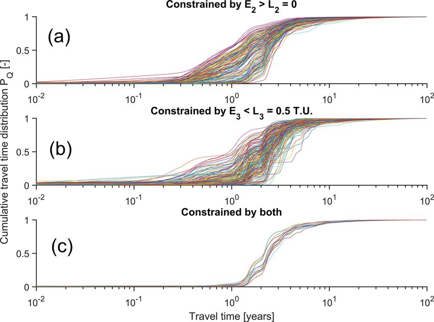
404                                                     N. B. Rodriguez et al.: Travel times from deuterium and tritium tracers

                                                                       near-stream soils, and by infiltration excess overland flow in
                                                                       the riparian area. The second peaks are generated by delayed
                                                                       lateral subsurface flow. The lateral fluxes are assumed higher
                                                                       at the PPSD/bedrock interface due to the hydraulic conduc-
                                                                       tivity contrasts (Glaser et al., 2016, 2019; Loritz et al., 2017).
                                                                       Lateral subsurface flows are, thus, accelerated when ground-
                                                                       water rises after a rapid vertical infiltration through the soils
                                                                       (Rodriguez and Klaus, 2019). The model based on travel
                                                                       times presented in this study was developed in a step-wise
                                                                       manner, based on this hypothesis of streamflow generation,
                                                                       and the consistency between simulated and observed δ 2 H
                                                                       points toward a robust representation of the key processes.
                                                                       Water flow paths and streamflow-generation processes in this
                                                                       catchment are, however, not completely resolved. Other stud-
                                                                       ies carried out in the Colpach catchment (containing the
                                                                       Weierbach) suggested that the first peaks are caused by a lat-
                                                                       eral subsurface flow through a highly conductive soil layer,
                                                                       and that second peaks are caused by groundwater flow in the
                                                                       bedrock (Angermann et al., 2017; Loritz et al., 2017). This is
                                                                       contrary to the conclusions from other studies in the Weier-
                                                                       bach catchment (Glaser et al., 2016, 2020), showing that the
                                                                       key processes are still under debate.

                                                                       2.2   Hydrometric and tracer data

                                                                       In this study, we use precipitation (J ; in mm h−1 ),
                                                                       ET (mm h−1 ), Q (mm h−1 ), and δ 2 H (‰) and 3 H (tri-
                                                                       tium units – TUs) measurements in precipitation (CP,2 and
                                                                       CP,3 , respectively) and streamflow (CQ,2 and CQ,3 , respec-
Figure 1. Map of the Weierbach catchment and its location in           tively). Here, the subscript 2 indicates deuterium (2 H) and the
Luxembourg. The weir is located at coordinates (5◦ 470 4400 E,         subscript 3 indicates tritium (3 H). The analysis in this study
49◦ 490 3800 N). SRS is the sequential rainfall sampler. AS is the     focuses on the period October 2015–October 2017 (Fig. 2).
stream autosampler. The elevation lines increase by 5 m, from          Details on the hydrometric data collection (J , ET, and Q),
460 m above sea level (a.s.l.) downstream close to the weir location
                                                                       and on the 2 H sample collection and analysis are given in
to 510 m a.s.l. at the northern catchment divide.
                                                                       Rodriguez and Klaus (2019).
                                                                          The 1088 stream grab samples analyzed for 2 H were
                                                                       instantaneous samples collected manually or automatically
bedrock that can be considered impervious. The climate is              with an autosampler (AS; Fig. 1), resulting in samples taken,
temperate and semi-oceanic. The flow regime is governed by             on average, every 15 h over October 2015–October 2017.
the interplay of seasonality between precipitation and evap-           These stream samples represent most flow conditions in the
otranspiration. Precipitation is fairly uniformly distributed          catchment in terms of frequency of occurrence (Fig. 3). The
over the year and averaged 953 mm yr−1 over 2006–2014                  525 precipitation samples analyzed for 2 H were collected ap-
(Pfister et al., 2017). The runoff coefficient over the same pe-       proximately every 2.5 mm rain increment (i.e., every 23 h on
riod is 50 %. Streamflow (Q) is double peaked during wetter            average) with a sequential rainfall sampler (SRS) and, in ad-
periods (Martínez-Carreras et al., 2016) and single peaked             dition, as cumulative bulk samples on an approximately bi-
during drier periods that normally occur in summer when                weekly basis (but ranging from 1 to 4 weeks in some occa-
evapotranspiration (ET) is high.                                       sions). Both the sequential rainfall samples and the cumu-
   Based on previous modeling (e.g., Fenicia et al., 2014;             lative bulk samples represent a precipitation-weighted aver-
Glaser et al., 2019) and experimental studies (e.g., Martínez-         age δ 2 H over different time intervals (approximately daily
Carreras et al., 2016; Juilleret et al., 2016; Scaini et al., 2017;    intervals for sequential rainfall samples and approximately
Glaser et al., 2018), Rodriguez and Klaus (2019) proposed a            biweekly intervals for bulk samples). The samples were an-
perceptual model of streamflow generation in the Weierbach             alyzed at the Luxembourg Institute of Science and Technol-
catchment. In this model, the first and flashy peaks of double-        ogy (LIST), using a Los Gatos Research (LGR) isotope wa-
peaked hydrographs are generated by precipitation falling              ter analyzer, yielding an analytical accuracy of 0.5 ‰ (equal
directly into the stream, by saturation excess flow from the           to the LGR standard accuracy) for 2 H and a precision-

Hydrol. Earth Syst. Sci., 25, 401–428, 2021                                               https://doi.org/10.5194/hess-25-401-2021
A comparison of catchment travel times and storage deduced from deuterium and tritium tracers using StorAge Selection functions
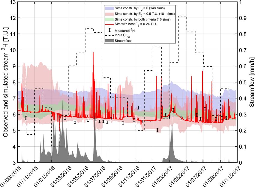
N. B. Rodriguez et al.: Travel times from deuterium and tritium tracers                                                                       405

Figure 2. Data used in this study – 3 H in precipitation (CP,3 ), the corresponding tritium activities accounting for radioactive decay un-
           ∗ ), δ 2 H in precipitation C
til 2017 (CP,3                                                                                      3
                                         P,2 (inset), precipitation J (inset), streamflow Q (inset), H measurements in the stream (CQ,3 – both
plots), and δ 2 H in the stream (CQ,2 ; inset). The period contained in the inset is represented as a rectangle in the bigger plot. The dashed line
visually represents the increasing trend in CP,3∗ that emerges as the effect of bomb peak tritium disappears (i.e., C (t − T ) stops decreasing
                                                                                                                        P,3
                                         ∗ (T , t) = C (t − T )e−αT starts decreasing with increasing T ).
approximately from the year 2000 on, so CP,3          P,3

                                                                            tion was not based on flows ranked by exceedance proba-
                                                                            bilities but rather on the streamflow time series itself. The
                                                                            selected samples represent various hydrological conditions
                                                                            (e.g., the beginning of a wet period after a long dry spell or
                                                                            small but flashy streamflow responses) based on data avail-
                                                                            able for this catchment (see Sect. 2 and Rodriguez and Klaus,
                                                                            2019). The 24 tritium samples cover a wide portion of the
                                                                            flow frequencies (see Fig. 3; all sampled flow conditions
                                                                            occurred more than 90 % of the time). This number of 3 H
                                                                            samples is one of the highest used in travel time studies
                                                                            (see Małoszewski and Zuber, 1993; Uhlenbrook et al., 2002;
                                                                            Stewart et al., 2007; Gallart et al., 2016; Gabrielli et al., 2018;
                                                                            Visser et al., 2019), and it is limited by the analytical costs.
                                                                            The samples were analyzed by the GNS Science water dat-
                                                                            ing laboratory (Lower Hutt, New Zealand), which provides
                                                                            high-precision tritium measurements using electrolytic en-
                                                                            richment and liquid scintillation counting (Morgenstern and
                                                                            Taylor, 2009). The precision of the stream samples varies
                                                                            from roughly 0.07 TU to roughly 0.3 TU, but it is usually
Figure 3. Distribution of stream samples (3 H and δ 2 H) along the
flow exceedance probability curve defined as the fraction of stream-        around 0.1 TU. 3 H in the precipitation was obtained for the
flows exceeding a given value over 2015–2017.                               Trier station (Global Network of Isotopes in Precipitation,
                                                                            GNIP, station; 60 km away from the Weierbach) until 2016
                                                                            from the WISER database of the International Atomic En-
                                                                            ergy Agency (IAEA; IAEA and WMO, 2019; Stumpp et al.,
maintained < 0.5 ‰ (quantified as 1 standard deviation of                   2014). The 2017 values were obtained from the radiology
the measured samples and standards).                                        group of the Bundesanstalt für Gewässerkunde (Schmidt
   The 24 stream samples analyzed for 3 H were instanta-                    et al., 2020). 3 H in precipitation before 1978 was calcu-
neous grab samples selected from manual biweekly sampling                   lated by regression with data from Vienna, Austria (Stew-
campaigns to cover various flow ranges. The manual selec-

https://doi.org/10.5194/hess-25-401-2021                                                      Hydrol. Earth Syst. Sci., 25, 401–428, 2021
A comparison of catchment travel times and storage deduced from deuterium and tritium tracers using StorAge Selection functions
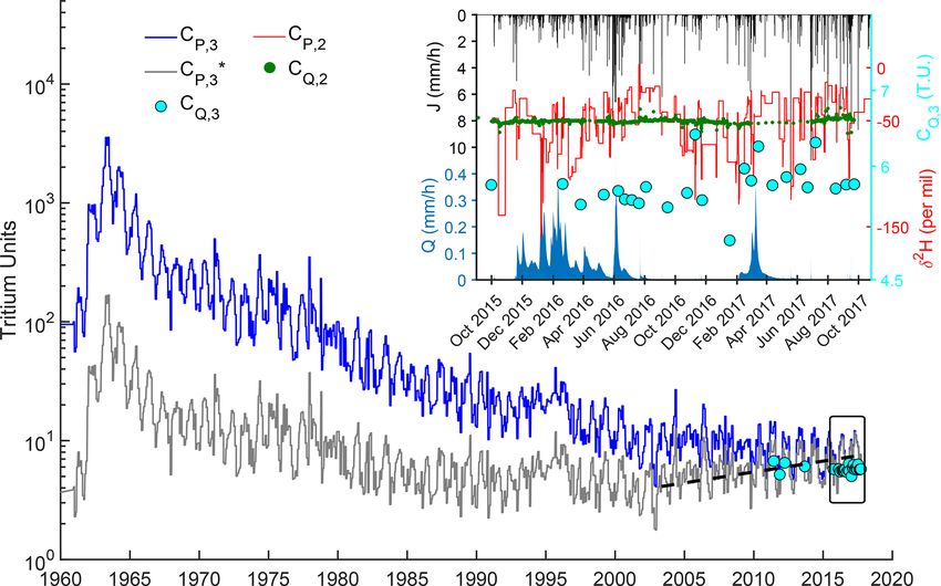
406                                                 N. B. Rodriguez et al.: Travel times from deuterium and tritium tracers

art et al., 2017). 3 H in precipitation obtained from the IAEA     at time t with travel time T (this parcel was in the inflow
corresponds to monthly integrated sampling made with an            at time t − T ). The concentrations in this equation need to
evaporation-free rain totalizer, as described in the GNIP sta-     be flux concentrations, i.e., representative of the tracer mass
tion operations manual.                                            fluxes in inflows and outflows (see Sect. 2.2). This equation is
   Since the stream grab samples were collected over a short       always true for the exact (usually unknown) TTD because it
time interval (seconds to minutes) using a weir, the associ-       simply expresses the fact that the stream concentration is the
ated concentrations, CQ,2 (t) and CQ,3 (t), represent the in-      volume-weighted arithmetic mean of the concentrations of
stantaneous value of the deuterium and tritium concentra-          the water parcels with different travel times at the outlet (the
tions in the stream at time t, equivalent to the concept of flux   weighting of tracer concentrations by hydrological fluxes is
                                                                                     ←
concentrations in Kreft and Zuber (1978) and Małoszewski           thus implicit in pQ (T , t)). Thus, contrary to most of the past
and Zuber (1982). For both 2 H and 3 H, the time series of         travel time studies using a steady-state version of Eq. (1),
tracer in precipitation was interpolated between two consec-       no weighting of the concentrations by fluxes is necessary
                                                                                                         ←
utive samples (e.g., A and B) as being equal to the value of       because the time-varying TTD pQ (T , t) already accounts
the next sample (i.e., B). This was necessary in order to ob-      for the time-varying fractions of precipitation not reaching
tain a continuous tracer input time series (required for Eq. (1)   the stream (due to either ET or storage; see Sect. 2.4) and
to work). For 2 H, the signal obtained from cumulative bulk        for time-varying streamflow rates. CP∗ (T , t) depends on T
samples was continuous by design and, thus, used as a base-        and t as separate variables if the tracer concentration of
line representing the steps of constant δ 2 H over 2 weeks         a water parcel in the catchment changes between injection
on average. Then, the discontinuous signal with higher fre-        time t − T and observation time t. For solutes like silicon
quency variations provided by the sequential rainfall sam-         and sodium, the concentration can increase with travel time
ples was inserted into the continuous baseline for the pe-         (Benettin et al., 2015a). For 3 H, radioactive decay with a con-
riods when sequential rainfall samples were available (this        stant α = 0.0563 yr−1 implies CP,3  ∗ (T , t) = C (t −T )e−αT ,
                                                                                                                    P,3
higher frequency signal is not continuous because of the pe-       where CP,3 (t − T ) is the concentration in precipitation mea-
riods of the absence of samples when the SRS failed). There-       sured at t − T . For 2 H, CP,2∗ (T , t) = C (t − T ). Thus, the
                                                                                                               P,2
fore, in this study, CP,2 (t) represents the instantaneous value   streamflow TTD simultaneously verifies Eqs. (2) and (3) as
of δ 2 H in precipitation at time t, equal to the precipitation-   follows:
weighted average value over varying time intervals. Also,
                                                                              Z+∞
CP,3 (t) represents the instantaneous value of 3 H in precip-                     ∗          ←
itation at time t, equal to the precipitation-weighted average     CQ,2 (t) =    CP,2 (T , t)pQ (T , t)dT
value over monthly intervals. Assuming uniform precipita-                    T =0
tion over the catchment, CP,2 (t) and CP,3 (t) are also equiv-                 Z+∞
                                                                                                 ←
alent to flux concentrations (Małoszewski and Zuber, 1982).                =        CP,2 (t − T )pQ (T , t)dT .                (2)
Since no measurements of J , Q, ET, and CP,2 are available
                                                                             T =0
before 2010, we periodically looped back their values from
                                                                               Z+∞
the period of October 2010–October 2015 for the time period                          ∗         ←
                                                                   CQ,3 (t) =       CP,3 (T , t)pQ (T , t)dT
before 2010 as a best estimate of their past values (Figs. S16
and S17). We aggregated the input data (J , ET, Q, CP,2 , and                T =0
CP,3 ) to a resolution 1t = 4 h, which is small enough to cap-                 Z+∞
                                                                                                        ←
ture the variability in the flows and tracers in the input and             =        CP,3 (t − T )e−αT pQ (T , t)dT .           (3)
simulate the variability in the flows and tracers in the output.             T =0

2.3   Mathematical framework                                       Practically, when measurements of 2 H and 3 H are used to in-
                                                                   versely deduce the TTD by using Eqs. (2) and (3), different
Mathematically, the streamflow TTD is related to the stream        TTDs may be found. These different TTDs may be called
tracer concentrations CQ (t), according to the following            ←         ←                               2      3
                                                                   p Q,2 and p Q,3 for instance, referring to H and H, respec-
Eq. (1):                                                           tively. To avoid introducing more variables and to avoid con-
                                                                                                         ←       ←
         Z+∞                                                       fusion, we do not use the names pQ,2 and pQ,3 , and we in-
                       ←                                           stead refer to the TTDs constrained by a given tracer using a
CQ (t) =    CP∗ (T , t)pQ (T , t)dT ,                       (1)                        ←
                                                                   common symbol pQ . We do this also to stress that the exact
         T =0
                                                                   (true) TTD must simultaneously verify both Eqs. (2) and (3),
                                                                                                   ←         ←
where T is the travel time (the age of water at the outlet),       and that two different TTDs pQ,2 and pQ,3 cannot physically
t is time of observation, CQ (t) is the stream tracer concentra-   exist. This is a fundamental difference from previous work
       ←
tion, pQ (probability distribution function – pdf) is the stream   that assumed two different TTDs, using for example Eq. (3)
backward TTD (Benettin et al., 2015b), and CP∗ (T , t) is the      for 3 H and another method for 2 H (the sine wave approach;
tracer concentration of the water parcel reaching the outlet       e.g., Małoszewski et al., 1983). The framework in this study

Hydrol. Earth Syst. Sci., 25, 401–428, 2021                                           https://doi.org/10.5194/hess-25-401-2021
A comparison of catchment travel times and storage deduced from deuterium and tritium tracers using StorAge Selection functions
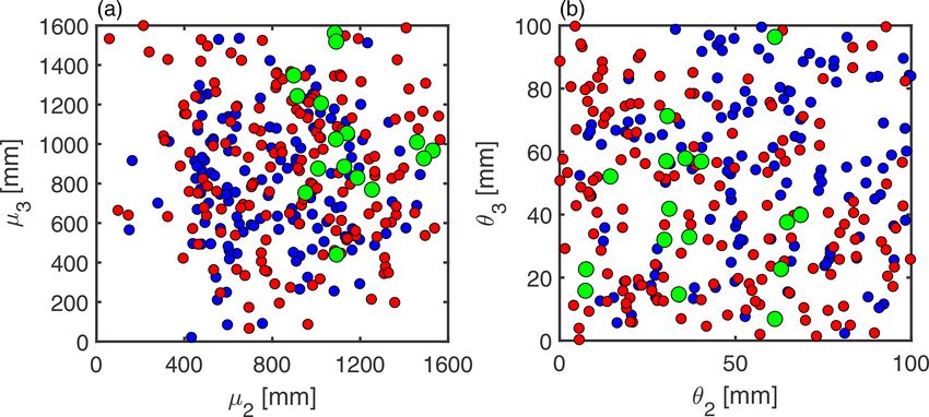
N. B. Rodriguez et al.: Travel times from deuterium and tritium tracers                                                           407

also uses the fact that the same functional form of stream-        The partial derivative with respect to travel time T ensures
flow TTD needs to simultaneously explain both tracers to be        the transition from cdf to pdf. Assuming a parameterized
valid, unlike previous work that used different TTD models         form for Q and ET , and calibrating their parameters us-
for different tracers (Stewart and Thomas, 2008).                  ing the framework defined in Sect. 2.3, yields time-varying
                                                                   TTDs constrained by the tracers in the outflows. In this study,
2.4   Transport model based on TTDs                                the parameters of Q are directly calibrated by using Eq. (1)
                                                                   for CQ . Since no tracer data CET are available, the param-
                                                                   eters of ET are indirectly deduced from Eq. (1) using the
Most of the previous travel time studies using tritium as-
                                                                   tracer measurements in streamflow only. This is made possi-
sumed steady-state flow conditions and an analytical shape
                                                                   ble by the indirect influence of ET on the tracer partition-
for the streamflow TTD and fitted the parameters of the an-
                                                                   ing between Q and ET and on the tracer mass balance (Ap-
alytical function using the framework described in Sect. 2.3.
                                                                   pendix A2).
In this study, the TTDs are unsteady (i.e., time varying or
                                                                      We assumed that ET is a function of only ST , and it is
transient) and cannot be analytically described. Still, they
                                                                   gamma distributed with a mean parameter µET (in millime-
can be calculated by numerically solving the master equation
                                                                   ters) and a scale parameter θET (in millimeters). Rodriguez
(Botter et al., 2011). This method has been applied in several
                                                                   and Klaus (2019) showed that, in the Weierbach catch-
recent studies (e.g., van der Velde et al., 2015; Harman, 2015;
                                                                   ment, a weighted sum of three components in the stream-
Benettin et al., 2017b) and is described in more detail by
                                                                   flow SAS function is more consistent with the superposition
Benettin and Bertuzzo (2018). The numerical method used
                                                                   of streamflow-generation processes (i.e., saturation excess
to solve this equation in this study is described by Rodriguez
                                                                   flow, saturation overland flow, and lateral subsurface flow;
and Klaus (2019). The biggest difference, compared to many
                                                                   see Sect. 2.1) than a single component. This means that Q is
previous travel time studies, is that time-varying TTDs can
                                                                   written as a weighted sum of three cdf’s (see Appendix A1;
be obtained from the master equation without using tracer
                                                                   Rodriguez and Klaus, 2019) as follows:
information (i.e., Eqs. 2 and 3). In this case, tracer equations
(Eqs. 2 and 3) simply become a constraint on the solutions
                                                                   Q (ST , t) = λ1 (t)1 (ST ) + λ2 (t)2 (ST ) + λ3 (t)3 (ST ) . (5)
found by solving the master equation.
   Essentially, the master equation is a water balance equa-
                                                                   λ1 (t), λ2 (t), and λ3 (t) are time-varying weights summing
tion in which storage and fluxes are labeled with age cat-
                                                                   to one. λ1 (t) is parameterized to sharply increase during
egories. The master equation is thus a partial differential
                                                                   flashy streamflow events, using parameters λ∗1 , f0 , Sth (in
equation. It expresses the fact that the amount of water in
                                                                   millimeters), and 1Sth (in millimeters; see Appendix A1).
storage, with a given residence time, changes with calendar
                                                                   λ2 (t) = λ2 is calibrated, and λ3 (t) is just deduced by dif-
time. This change is due to new water introduced by pre-
                                                                   ference. 1 is a cumulative uniform distribution over ST
cipitation J (t), water aging, and losses to catchment out-
                                                                   in [0, Su ] (with Su a parameter in millimeters). 1 repre-
flows ET(t) and Q(t). Solving the master equation requires
                                                                   sents the young water contributions associated with short
knowledge (or an assumption about the shape) of the SAS
                                                                   flow paths during flashy streamflow events. We chose rather
functions Q and ET of outflows Q and ET, which con-
                                                                   low values of λ∗1 (see Table 1), such that λ1 (t) is gener-
ceptually represent how likely it is that water ages in stor-
                                                                   ally the smallest weight (because λ1 (t) ≤ λ∗1 ). The lower
age (residence times) are to be present in the outflows at
                                                                   values of λ1 (t) compared to other weights are consistent
a given time. Solving the master equation yields the distri-
                                                                   with tracer data, suggesting limited contributions of event
bution of residence times in storage at every moment that
                                                                   water to streamflow (Martínez-Carreras et al., 2015; Wrede
can be represented in a cumulative form with age-ranked
                                                                   et al., 2015). 1 corresponds to the following processes in
storage ST . It is defined as the amount of water in storage
                                                                   the near-stream area: saturation excess flow, saturation over-
(e.g., 10 mm) younger than T (e.g., 1 year) at time t. T → ST
                                                                   land flow, and rain on the stream (Rodriguez and Klaus,
is just a mathematical change of a variable, and it has no
                                                                   2019). 2 and 3 are gamma distributed, with mean pa-
meaning respective to the location or depth of a water parcel
                                                                   rameters µ2 and µ3 (in millimeters) and scale parameters θ2
with a certain residence time in the catchment. By definition
                                                                   and θ3 (in millimeters), respectively. 2 and 3 represent
  lim ST = S(t), where S(t) is catchment storage. Q and
T →+∞                                                              older water that is always contributing to the stream. This
ET are functions of ST and cumulative distributions func-         older water consists of groundwater stored in the weathered
tions (cdf’s) for numerical convenience. SAS functions are         bedrock that flows laterally in the subsurface. Note that we
closely linked to TTDs, such that one can be found from the        used the same functional form of Q (ST , t) for 2 H and 3 H to
other using the following expression (here it has been used        keep the functional form of the TTDs consistent between the
for Q, but it is also valid for other outflows):                   tracers. Although composite SAS functions may consider-
                                                                   ably increase the complexity of the model compared to tradi-
←                ∂                                                tional SAS functions, they are necessary to account for differ-
p Q (T , t) =      Q (ST , t) .                            (4)    ent streamflow-generation processes (Rodriguez and Klaus,
                ∂T

https://doi.org/10.5194/hess-25-401-2021                                            Hydrol. Earth Syst. Sci., 25, 401–428, 2021
A comparison of catchment travel times and storage deduced from deuterium and tritium tracers using StorAge Selection functions
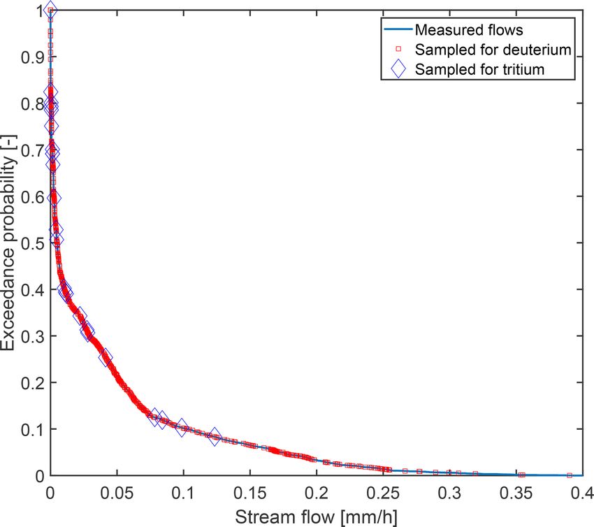
408                                                  N. B. Rodriguez et al.: Travel times from deuterium and tritium tracers

2019). These processes are potentially associated with con-            Unlike our previous modeling work in this catchment (Ro-
trasting flow path lengths and/or water velocities, hence the       driguez and Klaus, 2019), we fixed the initial storage in the
contrasting travel times. The accurate representation of these      model Sref (to 2000 mm). We did this to reduce the degrees of
contrasting travel times is most likely vital for reliable simu-    freedom when sampling the parameter space in order to limit
lations of stream chemistry (Rodriguez et al., 2020).               the impact of numerical errors on the calibration. These er-
                                                                    rors are due to the numerical truncation of Q (ST , t) when
2.5   Model initialization and numerical details                    a considerable part (e.g., a few percent) of its tail extends
                                                                    above S(t). This occurs when parameters µ2 , µ3 , θ2 , and
Numerically solving the master equation requires an estima-         θ3 are too large compared to Sref when the latter is also ran-
tion of catchment mobile storage S(t). Here, S(t) represents        domly sampled. Choosing a constant large value for Sref thus
the sum of dynamic (or active) storage and inactive (or pas-        guarantees the absence of truncation errors. Sref has little in-
sive) storage (Fenicia et al., 2010; Birkel et al., 2011; Soulsby   fluence on the storage deduced from travel times, since the
et al., 2011; Hrachowitz et al., 2013). In this study, the model    ages sampled from storage by streamflow are governed only
is initialized with storage S(t = 0) = Sref = 2000 mm. This         by µ2 , µ3 , θ2 , and θ3 . These parameters are independent
initial value is chosen to be large enough to sustain Q and ET      of Sref as long at it allows sufficiently old water to reside in
during drier periods and to store water that is sufficiently        storage, which is ensured by its large value and by the long
old to satisfy Eq. (1). S(t) is then simply deduced from the        spin-up period we used (100 years).
                                  Rt                                   The first step in the Monte Carlo procedure consisted of
water balance as S(t) = Sref + (J (x) − Q(x) − ET(x))dx.
                                x=0                                 randomly sampling parameters from the uniform prior dis-
The initial residence time distribution in storage pS (T , t) is    tributions with the ranges defined in Table 1. A total of
exponential with a mean of 1.7 years, the mean residence            12 096 sets of the 12 calibrated parameters were sampled
time (MRT) by Pfister et al. (2017). Initial conditions need        as a Latin hypercube (LHS; Helton and Davis, 2003). This
not be specified for the SAS functions, since these are di-         sampling technique has the advantages of a stratified sam-
rectly calculated from the initial state variables (ST (t = 0) =    pling technique and the simplicity and objectivity of a purely
           RT                                                       random sampling technique (Helton and Davis, 2003). It was
S(t = 0)      pS (x, t = 0)dx), assuming a parametric form          chosen to make sure that the parameter samples are as evenly
         x=0
and a set of parameter values. The model is then run with           distributed as possible, despite their relatively small number
the time steps 1t = 4 h and age resolution 1T = 8 h. In this        with respect to the high number of dimensions (due to com-
way, the computational cost is balanced with the resolution of      putational constraints enhanced by the required long spin-
the simulations in δ 2 H. A 100-year spin-up is used to numer-      up period). The model was then run over the 100-year spin-
ically allow the presence of water of up to 100 years old in        up followed by October 2015–October 2017, and its perfor-
storage and to avoid a numerical truncation of the TTDs. This       mance was evaluated over October 2015–October 2017. We
spin-up is also long enough to completely remove the impact         evaluated model performance in a multi-objective manner, by
of the initial conditions. This means that Sref and the initial     using separate objective functions for 2 H and 3 H. For deu-
residence time distribution in storage do not influence the re-     terium, we used the Nash–Sutcliffe efficiency (NSE) as fol-
sults over October 2015–October 2017. ET(t) is taken to be          lows:
equal to potential evapotranspiration PET(t), except that it                      N2                           2
                                                                                       CQ,2 (tk ) − δ 2 H (tk )
                                                                                  P
tends nonlinearly towards 0 (using a constant smoothing pa-
rameter n) when storage S(t) decreases below Sroot (in mil-                       k=1
                                                                    E2 = 1 −                                        ,           (6)
                                                                                    N2                        2
limeters) and where Sroot is a parameter accounting for the
                                                                                         
                                                                                          δ 2 H (tk ) − δ 2 H
                                                                                    P
water amount accessible by ET (Appendix A2).                                       k=1

2.6   Model calibration                                             where N2 = 1016 is the number of deuterium observations
                                                                    in the stream. For tritium, we used the mean absolute error
The parameters of the SAS functions and the other model             (MAE) as follows:
parameters were calibrated using a Monte Carlo technique.
                                                                           N3
In total, 12 parameters were calibrated (Table 1). The ini-                X
                                                                                  CQ,3 tj − 3 H tj ,
                                                                                                 
                                                                    E3 =                                                        (7)
tial ranges were selected based on parameter feasible val-                 j =1
ues (e.g., f0 between 0 and 1 by definition), on previous
estimations (e.g., Sth ), on hydrological data (e.g., Su and        where N3 = 24 is the number of tritium observations in the
1Sth deduced from average precipitation depths), and on             stream. We used the MAE for tritium because it is com-
initial tests done on the parameter ranges (e.g., µ and θ ).        mon to report errors in TU and because of the limited vari-
These ranges allow a wide range of shapes of SAS functions,         ance in stream 3 H (due to the limited number of samples
while minimizing numerical errors (occurring, for example,          and the low variability), making the NSE less appropriate
for ST > S(t)).                                                     (Gallart et al., 2016). The behavioral parameter sets that are

Hydrol. Earth Syst. Sci., 25, 401–428, 2021                                               https://doi.org/10.5194/hess-25-401-2021
N. B. Rodriguez et al.: Travel times from deuterium and tritium tracers                                                                                                                  409

Table 1. Model parameters.

  Symbol         Type               Unit       Initial range        Descriptiona
  Sth            Calibrated         mm             [20, 200]        Storage threshold relative to Smin separating dry and wet periods
  1Sth           Calibrated         mm              [0.1, 20]       Threshold in short-term storage changes identifying first peaks in hydrographs
  Su             Calibrated         mm                [1, 50]       Range of the uniformly distributed 1
  f0             Calibrated         –                   [0, 1]      Young water coefficient for the dry periods
  λ∗1            Calibrated         –                 [0, 1]b       Maximum value of the weight λ1 (t)
  λ2             Calibrated         –                   [0, 1]      Constantc value of the weight λ2 (t)
  µ2             Calibrated         mm             [0, 1600]        Mean parameter of the gamma-distributed 2
  θ2             Calibrated         mm               [0, 100]       Scale parameter of the gamma-distributed 2
  µ3             Calibrated         mm             [0, 1600]        Mean parameter of the gamma-distributed 3
  θ3             Calibrated         mm               [0, 100]       Scale parameter of the gamma-distributed 3
  µET            Calibrated         mm             [0, 1600]        Mean parameter of the gamma-distributed ET
  θET            Calibrated         mm               [0, 100]       Scale parameter of the gamma-distributed ET
  Sroot          Constant           mm                   150        Water amount accessible by ET
  m              Constant           –                   1000        Smoothing parameter for the calculation of λ1 (t)
  n              Constant           –                     20        Smoothing parameter for the calculation of ET(t) from PET(t)
  1t ∗           Constant           h                      8        Width of the moving time window used to calculate short-term storage variations 1S(t)
a Details about the equations involving these parameters are given in Appendix A1 and in Rodriguez and Klaus (2019). b λ∗ is, in fact, uniformly sampled between 0 and
                                                                                                                               1
                            3
                               λk (t) = 1. This also ensures that values close to 0 are more often sampled than values close to 1 for λ∗1 . c λ1 (t) varies, λ2 is constant, and λ3 (t) varies,
                           P
1 − λ2 ≤ 1 to ensure that
                          n=1
and it is deduced using λ3 (t) = 1 − λ2 − λ1 (t).

used for uncertainty calculations and further analysis were                                        and posterior parameter distributions, using the Shannon en-
selected based on threshold values L2 and L3 for the perfor-                                       tropy H as follows:
mance measures E2 and E3 , respectively (Beven and Binley,
                                                                                                               nI
1992). Parameter sets were considered behavioral for deu-
                                                                                                             X
                                                                                                   H X|i H = −    f (Ik ) log2 f (Ik ) .                                                  (8)
terium simulations, if E2 > L2 = 0, and behavioral for tri-                                                                k=1
tium simulations, if E3 < L3 = 0.5 TU. We subsequently re-
fer to these parameter sets and corresponding simulations as                                       In this equation, the parameter X (e.g., µ2 ) takes values
constrained by deuterium, constrained by tritium, and con-                                         (e.g., 125 mm) falling in intervals Ik (e.g., [100, 150] mm)
strained by both when both performance criteria were used.                                         that do not intersect each other and which union ∪nk=1      I
                                                                                                                                                                  Ik
We chose these constraints to obtain reasonable model fits to                                      equals IX , the total interval of values on which X is defined
the data, to obtain a comparable number of behavioral param-                                       (e.g., [50, 500] mm). The definitions of the nI intervals Ik for
eter sets for 2 H and 3 H, and to maximize the amount of infor-                                    each parameter depend on the binning of the parameter val-
mation gained about the parameters when adding a constraint                                        ues (given in Table 2). The distribution f defines the proba-
on the model performance for a tracer. This information gain                                       bility of the parameter X to be in a certain state (i.e., to take
was assessed with the Kullback–Leibler divergence DKL be-                                          a value falling in an interval Ik ) when constrained by the cri-
tween the parameter distributions inferred from various com-                                       terion E2 > L2 (i = 2) or E3 < L3 (i = 3) (posterior distribu-
binations of constraints L2 and L3 (Sect. 2.7).                                                    tion) or none of those (prior distribution). f can also be cal-
                                                                                                   culated for a combination of these criteria (H(X|(2 H∩ 3 H))).
2.7     Information contents of 2 H and 3 H                                                        When using the logarithm of base 2, H is expressed in bits of
                                                                                                   information contained in the distribution f . The uniform dis-
                                                                                                   tribution over IX has the maximum possible entropy. Lower
Loritz et al. (2018, 2019) recently used information theory to
                                                                                                   values of H thus indicate that the distribution is not flat;
detect the hydrological similarity between hillslopes of the
                                                                                                   hence, it is less uncertain than the uniform prior distribution.
Colpach catchment and to compare topographic indexes in
                                                                                                   In general, lower values of H indicate lower parameter un-
the Attert catchment in Luxembourg. Thiesen et al. (2019)
                                                                                                   certainty. Lower values of H for the posteriors also indicate
used information theory to build an efficient predictor of
                                                                                                   that information on travel times was extracted from the tracer
rainfall–runoff events. In this study, we leverage information
                                                                                                   time series. We used the Kullback–Leibler divergence DKL
theory to evaluate our model parameter uncertainty (Beven
                                                                                                   to precisely evaluate the information gain from prior to pos-
and Binley, 1992) and to assess the added value of δ 2 H
                                                                                                   terior distributions as follows:
and 3 H tracers for information gains on travel times. First,
we calculated the expected information content of the prior

https://doi.org/10.5194/hess-25-401-2021                                                                                  Hydrol. Earth Syst. Sci., 25, 401–428, 2021
410                                                 N. B. Rodriguez et al.: Travel times from deuterium and tritium tracers

                nI
            X                 f (Ik )
DKL X|i H, X =     f (Ik ) log2         ,                   (9)
               k=1
                                g (Ik )

where f is the posterior distribution constrained by E2 > L2
and/or E3 < L3 , and g is the prior distribution. DKL is ex-
pressed in bits of information gained when the knowledge
about a parameter distribution is updated by using tracer data.
Summing the DKL (X|i H, X) for all the parameters and for a
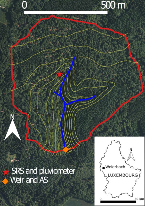
given tracer (i = 2 or i = 3) yields the total amount of infor-    Figure 4. Distributions of SAS function mean (µ; a) and scale (θ ; b)
mation learned on travel times from that tracer. We also used      behavioral parameters directly controlling the selection of longer
the Kullback–Leibler divergence DKL to evaluate the gain of        travel times by streamflow, constrained by deuterium (148 blue
information when 3 H is used in addition to 2 H to constrain       dots) or tritium (181 red dots) or both (16 green dots).
model predictions, or vice versa, in the following:
                            nI
                      X                 f (Ik )
DKL X| 2 H ∩ 3 H , X|i H =     f (Ik ) log2         , (10)         the gamma components in Q . These parameters thus have
                                            g (Ik )
                           k=1                                     a direct influence on the catchment storage inferred via age-
                                                                   ranked storage ST . The distributions of µ2 , θ2 , µ3 , and θ3 are
where f is the posterior distribution constrained by E2 > L2
                                                                   clearly not uniform. The distributions of the other parameters
and E3 < L3 , and g is the posterior distribution constrained
                                                                   are provided in the Supplement (Figs. S12 and S13). Most
only by E2 > L2 (i = 2) or only by E3 < L3 (i = 3). DKL is
                                                                   distributions are not uniform, indicating that the parameters
expressed in bits of information gained when the knowledge
                                                                   are identifiable.
about a parameter posterior distribution is updated by adding
                                                                      Essentially, the results (Table 2 and Fig. 4) reveal that the
another tracer. Calculating DKL also requires binning the pa-
                                                                   parameter ranges decreased by adding information on 2 H
rameter values to define the intervals Ik and calculate the dis-
                                                                   or 3 H or both. This effect is particularly noticeable for f0
tributions f and g. The binning for each parameter (Table 2)
                                                                   and λ∗1 , which saw their upper boundary decrease, and for µ2
was chosen such that the resulting histograms visually re-
                                                                   and µ3 , which saw their lower boundary increase consid-
veal the underlying structure of the parameter values, while
                                                                   erably. These results also show that the posterior distribu-
avoiding uneven features and irregularities (e.g., very spiky
                                                                   tions depart from the uniform prior distributions when con-
histograms).
                                                                   sidering 2 H alone or 3 H alone (i.e., H(X|i H) < H(X) and
                                                                   DKL (X|i H, X) > 0 in Table 2). This effect is not very pro-
3     Results                                                      nounced for most parameters, but it is clearly visible for λ∗1 ,
                                                                   µ2 and µ3 (e.g., uneven distributions of points in Fig. 4),
3.1    Calibration results                                         and for µET . The posterior distributions become considerably
                                                                   narrower when both tracers are considered, since H(X|(2 H∩
A total of 148 parameter sets were behavioral for deuterium        3 H)) is much lower than H(X), which is visually represented

simulations, with E2 ranging from L2 = 0 to 0.24. A total          by the distribution of points tending to cluster towards a cor-
of 181 parameter sets were behavioral for tritium simula-          ner in Fig. 4. Generally, more was learned about the likely pa-
tions, with E3 ranging from 0.24 to L3 = 0.5 TU. Addition-         rameter values by adding a constraint on 2 H simulations after
ally, 16 parameter sets were behavioral for both tritium and       constraining 3 H simulations to the opposite (i.e., generally
deuterium simulations, with E2 ranging from L2 = 0 to 0.19         DKL (X(2 H ∩ 3 H), X|3 H) ≥ DKL (X|(2 H ∩ 3 H), X|2 H)). No-
and E3 ranging from 0.36 to L3 = 0.5 TU. These solutions           ticeable exceptions to this are the parameters µ2 , θ2 , and θ3 ,
show that a reasonable agreement between the model fit to          which are more related to the longer travel times in stream-
2 H and the model fit to 3 H can be found.                         flow and to catchment storage than the other parameters.
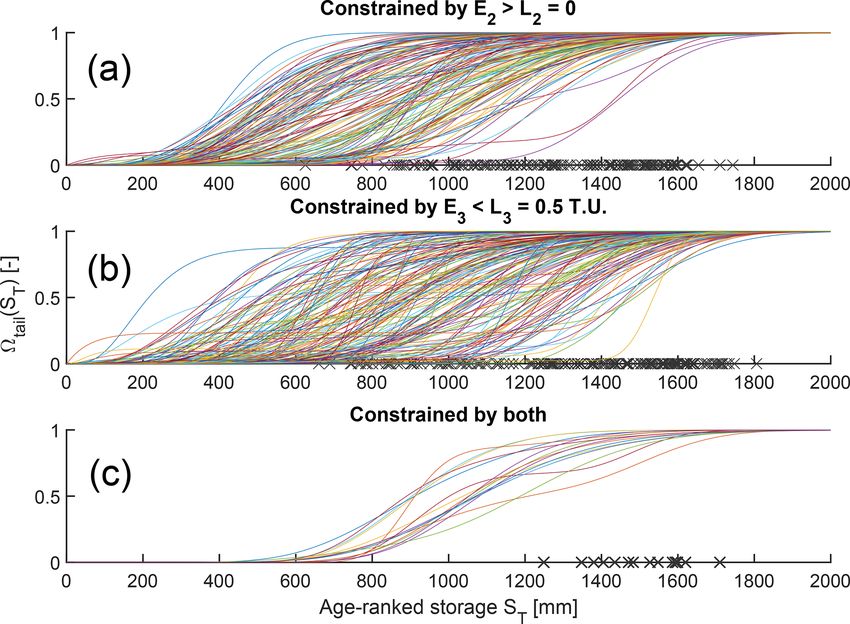
   The behavioral posterior parameter distributions con-              Simulations of stream δ 2 H captured both the slow and
strained by deuterium or tritium or by both generally had          the fast dynamics of the observations when constrained by
similar ranges to their prior distributions, except, notably,      E2 > 0 (blue bands and blue curve in Fig. 5a), although
for µ2 , θ2 , µ3 , and θ3 (Table 2). To assess the reduction in    some variability is not fully reproduced. The Nash–Sutcliffe
parameter uncertainty, we calculated and compared the en-          efficiency (E2 ) is limited to 0.24 despite visually satisfy-
tropy of the prior and of the posterior distributions (Table 2).   ing simulations (Sect. 4.4.2). Most flashy responses in δ 2 H
A visual inspection of the posterior distributions was also        (associated with flashy streamflow responses) were repro-
made. Here, we show only the parameters µ2 , θ2 , µ3 , and θ3      duced to some extent by the behavioral simulations (the
(Fig. 4) that directly control the range of longer travel times    very thin peaks of the blue bands in Fig. 5a; more visi-
in streamflow, since they act mostly on the right-hand tail of     ble in Figs. S1–S9 in the Supplement). Nevertheless, about

Hydrol. Earth Syst. Sci., 25, 401–428, 2021                                            https://doi.org/10.5194/hess-25-401-2021
N. B. Rodriguez et al.: Travel times from deuterium and tritium tracers                                                                                                                                                                                                                                                                                                                                                                                                                        411

                                                                                                                                                                                                                                                                                                                                                                                                                                   3 % of δ 2 H data points were visibly underestimated, point-

                                                                                                                                  mm
                                                                                                                              [1, 99]
                                                                                                                             [1, 100]
                                                                                                                              [3, 98]
                                                                                                                       [0 : 10 : 100]
                                                                                                                                 3.32
                                                                                                                                 3.24
                                                                                                                                 3.22
                                                                                                                                 2.48
                                                                                                                                 0.09
                                                                                                                                 0.10
                                                                                                                                 0.84
                                                                                                                                 0.72
                                                                                                                                 0.75
                                                                                                           θET
                                                                                                                                                                                                                                                                                                                                                                                                                                   ing at a partial limitation of the composite SAS functions
                                                                                                                                                                                                                                                                                                                                                                                                                                   to simulate the variability in the streamflow TTD at these
                                                                                                                                                                                                                                                                                                                                                                                                                                   few instances (see Sect. 4.4.2). Behavioral simulations that
                                                                                                                                   mm                                                                                                                                                                                                                                                                                              were selected using the other performance criterion instead
                                                                                                                             [51, 926]
                                                                                                                              [0, 959]
                                                                                                                             [51, 120]
                                                                                                                       [0 : 50 : 1600]
                                                                                                                                     5
                                                                                                                                  2.77
                                                                                                                                  1.53
                                                                                                                                   0.7
                                                                                                                                  2.22
                                                                                                                                  3.45
                                                                                                                                  4.30
                                                                                                                                  1.29
                                                                                                                                  2.04
                                                                                                           µET

                                                                                                                                                                                                                                                                                                                                                                                                                                   (E3 < 0.5 TU; red bands in Fig. 5) did not match the δ 2 H ob-
                                                                                                                                                                                                                                                                                                                                                                                                                                   servations well. This shows that 3 H contains some informa-
                                                                                                                                                                                                                                                                                                                                                                                                                                   tion on travel times that is not in common with 2 H. Yet, these
                                                                                                                                                                                                                                                                                                                                                                                                                                   behavioral simulations are able to match all observed δ 2 H
                                                                                                                                  mm
                                                                                                                             [2, 100]
                                                                                                                             [0, 100]
                                                                                                                              [7, 96]
                                                                                                                       [0 : 10 : 100]
                                                                                                                                 3.32
                                                                                                                                 3.23
                                                                                                                                 3.25
                                                                                                                                 2.75
                                                                                                                                 0.10
                                                                                                                                 0.07
                                                                                                                                 0.57
                                                                                                                                 0.48
                                                                                                                                 0.37
                                                                                                           θ3

                                                                                                                                                                                                                                                                                                                                                                                                       KL are expressed in bits.
                                                                                                                                                                                                                                                                                                                                                                                                                                   flashy responses in amplitude, suggesting that, like δ 2 H, 3 H
                                                                                                                                                                                                                                                                                                                                                                                                                                   contains information on young water contributions to stream-
                                                                                                                                                                                                                                                                                                                                                                                                                                   flow (Sect. 4.3). Additionally, δ 2 H simulations that were con-
                                                                                                                                                                                                                                                                                                                                                                                                                                   strained by both criteria (green bands) have a smaller vari-
                                                                                                                                    mm
                                                                                                                             [21, 1561]
                                                                                                                             [67, 1600]
                                                                                                                           [440, 1561]
                                                                                                                       [0 : 100 : 1600]
                                                                                                                                      4
                                                                                                                                   3.59
                                                                                                                                   3.83
                                                                                                                                   2.91
                                                                                                                                   0.41
                                                                                                                                   0.17
                                                                                                                                   1.10
                                                                                                                                   0.75
                                                                                                                                   0.84
                                                                                                           µ3

                                                                                                                                                                                                                                                                                                                                                                                                                                   ability than those constrained only by E2 > 0, suggesting

                                                                                                                                                       a Binning is indicated as [a : b : c], where a is the left edge of the first bin, b is the bin width, and c is the right edge of the last bin. For instance, [7 : 2 : 11] indicates data sorted with the two bins [7, 9] and [9, 11]. b H and D
                                                                                                                                                                                                                                                                                                                                                                                                                                   that 3 H contains some information that is common with 2 H.
                                                                                                                                                                                                                                                                                                                                                                                                                                       Simulations of stream 3 H generally matched the obser-
                                                                                                                                                                                                                                                                                                                                                                                                                                   vations better in 2017 than before 2017 (red bands and red
                                                                                                                                                                                                                                                                                                                                                                                                                                   curve in Fig. 6). Some simulations (red bands) nevertheless
                                                                                                                                  mm
                                                                                                                             [6, 100]
                                                                                                                             [0, 100]
                                                                                                                              [7, 69]
                                                                                                                       [0 : 10 : 100]
                                                                                                                                 3.32
                                                                                                                                 3.25
                                                                                                                                 3.25
                                                                                                                                 2.18
                                                                                                                                 0.07
                                                                                                                                 0.07
                                                                                                                                 1.14
                                                                                                                                 1.03
                                                                                                                                 0.91
                                                                                                           θ2

                                                                                                                                                                                                                                                                                                                                                                                                                                   matched the observations before 2017 relatively well. Simi-
                                                                                                                                                                                                                                                                                                                                                                                                                                   lar to δ 2 H simulations, both the slow and the fast tracer re-
                                                                                                                                                                                                                                                                                                                                                                                                                                   sponses seemed necessary to reproduce the variability in 3 H
                                                                                                                                    mm
                                                                                                                           [149, 1530]
                                                                                                                             [58, 1564]
                                                                                                                           [897, 1530]
                                                                                                                       [0 : 100 : 1600]
                                                                                                                                      4
                                                                                                                                   3.44
                                                                                                                                   3.73
                                                                                                                                   2.48
                                                                                                                                   0.56
                                                                                                                                   0.27
                                                                                                                                   1.52
                                                                                                                                   1.23
                                                                                                                                   1.08
                                                                                                           µ2

                                                                                                                                                                                                                                                                                                                                                                                                                                   observations (especially in 2017), although additional stream
                                                                                                                                                                                                                                                                                                                                                                                                                                   samples would be needed to confirm that the model is ac-
                                                                                                                                                                                                                                                                                                                                                                                                                                   curate between the current measurement points. The higher
                                                                                                                                                                                                                                                                                                                                                                                                                                   stream 3 H values in 2017 that were better reproduced by the
                                                                                                                                                                                                                                                                                                                                                                                                                                   model correspond to an extended dry period during which
                                                                                                                                   –
                                                                                                                              [0, 1]
                                                                                                                              [0, 1]
                                                                                                                            [0.1, 1]
                                                                                                                       [0 : 0.1 : 1]
                                                                                                                               3.32
                                                                                                                                3.2
                                                                                                                               3.24
                                                                                                                               2.91
                                                                                                                               0.12
                                                                                                                               0.08
                                                                                                                               0.41
                                                                                                                               0.27
                                                                                                                               0.34
                                                                                                           λ2
       Table 2. Parameter ranges and information measures before and after calibration to isotopic data.

                                                                                                                                                                                                                                                                                                                                                                                                                                   streamflow responses were mostly flashy and short-lasting
                                                                                                                                                                                                                                                                                                                                                                                                                                   hydrographs. The 3 H values in 2017 were closer to precip-
                                                                                                                                                                                                                                                                                                                                                                                                                                   itation 3 H, mostly around 10 TU (see also Fig. S15). The
                                                                                                                                    –
                                                                                                                            [0, 0.76]
                                                                                                                            [0, 0.92]
                                                                                                                            [0, 0.76]
                                                                                                                       [0 : 0.05 : 1]
                                                                                                                                 3.71
                                                                                                                                 2.97
                                                                                                                                 3.23
                                                                                                                                 2.65
                                                                                                                                 0.27
                                                                                                                                 0.13
                                                                                                                                 0.60
                                                                                                                                 0.36
                                                                                                                                 0.33
                                                                                                           λ∗1

                                                                                                                                                                                                                                                                                                                                                                                                                                   stream reaction to those higher values suggests a consider-
                                                                                                                                                                                                                                                                                                                                                                                                                                   able influence of recent rainfall events on the stream. Steady-
                                                                                                                                                                                                                                                                                                                                                                                                                                   state TTD models relying only on tritium decay would prob-
                                                                                                                                                                                                                                                                                                                                                                                                                                   ably struggle to simulate these fast responses. This also sug-
                                                                                                                                   –
                                                                                                                              [0, 1]
                                                                                                                              [0, 1]
                                                                                                                          [0, 0.82]
                                                                                                                       [0 : 0.1 : 1]
                                                                                                                               3.32
                                                                                                                               3.22
                                                                                                                                3.3
                                                                                                                               2.91
                                                                                                                               0.10
                                                                                                                               0.02
                                                                                                                               0.42
                                                                                                                                0.3
                                                                                                                               0.42
                                                                                                           f0

                                                                                                                                                                                                                                                                                                                                                                                                                                   gests a stronger influence of old water in 2016 than in 2017
                                                                                                                                                                                                                                                                                                                                                                                                                                   (see Sect. 4.4.2). Simulations constrained by deuterium (blue
                                                                                                                                                                                                                                                                                                                                                                                                                                   bands) tended to overestimate stream 3 H. Simulations con-
                                                                                                                               mm
                                                                                                                         [1.4, 50]
                                                                                                                           [1, 50]
                                                                                                                          [11, 49]
                                                                                                                       [0 : 5 : 50]
                                                                                                                              3.32
                                                                                                                              3.29
                                                                                                                              3.31
                                                                                                                              2.53
                                                                                                                              0.04
                                                                                                                              0.01
                                                                                                                              0.76
                                                                                                                              0.75
                                                                                                                                0.8
                                                                                                           Su

                                                                                                                                                                                                                                                                                                                                                                                                                                   strained by both criteria (green bands) worked well in 2017,
                                                                                                                                                                                                                                                                                                                                                                                                                                   but they overestimated stream 3 H before 2017. Similar to
                                                                                                                                                                                                                                                                                                                                                                                                                                   δ 2 H simulations, this suggests that 2 H and 3 H have com-
                                                                                                                                                                                                                                                                                                                                                                                                                                   mon but also distinct information contents on travel times.
                                                                                                                               mm
                                                                                                                        [0.14, 20]
                                                                                                                         [0.1, 20]
                                                                                                                        [0.17, 20]
                                                                                                                       [0 : 2 : 20]
                                                                                                                              3.32
                                                                                                                              3.27
                                                                                                                                3.3
                                                                                                                              2.95
                                                                                                                              0.05
                                                                                                                              0.02
                                                                                                                              0.37
                                                                                                                              0.36
                                                                                                                              0.36
                                                                                                           1Sth

                                                                                                                                                                                                                                                                                                                                                                                                                                   The tendency of the model constrained by deuterium and/or
                                                                                                                                                                                                                                                                                                                                                                                                                                   by tritium to overestimate the tritium content in streamflow
                                                                                                                                                                                                                                                                                                                                                                                                                                   suggests a nonnegligible influence of the isotopic partition-
                                                                                                                                   mm
                                                                                                                            [21, 196]
                                                                                                                            [20, 200]
                                                                                                                            [25, 177]
                                                                                                                       [20 : 20 : 200]
                                                                                                                                  3.17
                                                                                                                                  3.12
                                                                                                                                   3.1
                                                                                                                                  2.52
                                                                                                                                  0.05
                                                                                                                                  0.07
                                                                                                                                  0.64
                                                                                                                                  0.39
                                                                                                                                  0.48
                                                                                                           Sth

                                                                                                                                                                                                                                                                                                                                                                                                                                   ing of inputs between Q and ET (Sect. 4.4.2; Appendix A2;
                                                                                                                                                                                                                                                                                                                                                                                                                                   Fig. S15).

                                                                                                                                                                                                                                                                                                                                                                                                                                   3.2   Storage and travel time results
                                                                                                                       Range for E2 > L2 and E3 < L3

                                                                                                                                                                                                                                                                                                                                                                                                                                                                                           ←
                                                                                                                                                                                                                                                                                                                                                                                                                                   For each behavioral parameter set, we calculated P Q (T ),
                                                                                                                       DKL (X|(2 H ∩ 3 H), X|2 H)
                                                                                                                       DKL (X|(2 H ∩ 3 H), X|3 H)

                                                                                                                                                                                                                                                                                                                                                                                                                                   the average streamflow TTD weighted by Q(t) (over 2015–
                                                                                                                       DKL (X|(2 H ∩ 3 H), X)
                                                                                                                       Range for E2 > L2
                                                                                                                       Range for E3 < L3

                                                                                                                                                                                                                                                                                                                                                                                                                                   2017) in cumulative form (Fig. 7). Visually, there are no
                                                                                                                       H(X|(2 H ∩ 3 H))

                                                                                                                                                                                                                                                                                                                                                                                                                                                                   ←
                                                                                                                       DKL (X|2 H, X)
                                                                                                                       DKL (X|3 H, X)

                                                                                                                                                                                                                                                                                                                                                                                                                                   striking differences between P Q (T ) constrained by deu-
                                                                                                                                                                                                                                                                                                                                                                                                                                   terium or by tritium, except a slightly wider spread for sim-
                                                                                                           Parameter

                                                                                                                       H(X|2 H)
                                                                                                                       H(X|3 H)
                                                                                                                       Binninga

                                                                                                                                                                                                                                                                                                                                                                                                                                                                           ←
                                                                                                                       H(X)b

                                                                                                                                                                                                                                                                                                                                                                                                                                   ulations constrained by tritium. The P Q (T ) constrained by
                                                                                                                       Unit

                                                                                                                                                                                                                                                                                                                                                                                                                                   both tracers clearly differ. The associated curves (Fig. 7c)

https://doi.org/10.5194/hess-25-401-2021                                                                                                                                                                                                                                                                                                                                                                                                           Hydrol. Earth Syst. Sci., 25, 401–428, 2021
You can also read